Three Techniques for Rendering Generalized Depth of Field Effects Todd J. Kosloff∗ Computer Science Division, University of California, Berkeley, CA 94720 Brian A. Barsky† Computer Science Division and School of Optometry, University of California, Berkeley, CA 94720 Post-process methods are fast, sometimes to the point of real-time [13, 17, 9], but generally do not share the same image quality as distributed ray tracing. A full literature review of depth of field methods is beyond the scope of this paper, but the interested reader should consult the following surveys: [1, 2, 5]. Kosara [8] introduced the notion of semantic depth of field, a somewhat similar notion to generalized depth of field. Semantic depth of field is non-photorealistic depth of field used for visualization purposes. Semantic depth of field operates at a per-object granularity, allowing each object to have a different amount of blur. Generalized depth of field, on the other hand, goes further, allowing each point in space to have a different blur value. Generalized depth of field is more useful than semantic depth of field in that generalized depth of field allows per-pixel control over blur, whereas semantic depth of field only allows per-object control. Heat diffusion has previously been shown to be useful in depth of field simulation, by Bertalmio [3] and Kass [7]. However, they simulated traditional depth of field, not generalized depth of field. We introduced 1 Background and Previous Work generalized depth of field via simulated heat diffusion in 1.1 Simulated Depth of Field A great deal of work [10]. For completeness, the present work contains one has been done in rendering realistic (non-generalized) section dedicated to the heat diffusion method. Please depth of field effects, e.g. [4, 6, 12, 15, 13, 17]. see [10] for complete details. Distributed ray tracing [4] can be considered a gold standard; at great computational cost, highly accurate 1.2 Terminology The purpose of this section is to simulations of geometric optics can be obtained. For explain certain terms that are important in discussions each pixel, a number of rays are chosen to sample of simulated depth of field. Perhaps the most fundamental concept is that of the the aperture. Accumulation buffer methods [6] provide essentially the same results of distributed ray tracing, point spread function, or PSF. The PSF is the blurred but render entire images per aperture sample, in order image of a single point of light. The PSF completely characterizes the appearance of blur. In the terminology to utilize graphics hardware Both distributed ray tracing and accumulation of linear systems, the PSF is the impulse response of buffer methods are quite expensive, so a variety of faster the lens. Photographers use the Japanese word bokeh post-process methods have been created [12, 15, 2]. to describe the appearance of the out-of-focus parts of a Post-process methods use image filters to blur images photograph. Different PSFs will lead to different bokeh. originally rendered with everything in perfect focus. Typical high-quality lenses have a PSF shaped like their diaphragm, i.e. circles or polygons. On the other ∗ e-mail:
[email protected] hand, computer generated images often use Gaussian Abstract
Depth of field refers to the swath that is imaged in sufficient focus through an optics system, such as a camera lens. Control over depth of field is an important artistic tool that can be used to emphasize the subject of a photograph. In a real camera, the control over depth of field is limited by the laws of physics and by physical constraints. Depth of field has been rendered in computer graphics, but usually with the same limited control as found in real camera lenses. In this paper, we generalize depth of field in computer graphics by allowing the user to specify the distribution of blur throughout a scene in a more flexible manner. Generalized depth of field provides a novel tool to emphasize an area of interest within a 3D scene, to select objects from a crowd, and to render a busy, complex picture more understandable by focusing only on relevant details that may be scattered throughout the scene. We present three approaches for rendering generalized depth of field based on nonlinear distributed ray tracing, compositing, and simulated heat diffusion. Each of these methods has a different set of strengths and weaknesses, so it is useful to have all three available. The ray tracing approach allows the amount of blur to vary with depth in an arbitrary way. The compositing method creates a synthetic image with focus and aperture settings that vary per-pixel. The diffusion approach provides full generality by allowing each point in 3D space to have an arbitrary amount of blur.
† e-mail:
[email protected]
42
Copyright © by SIAM. Unauthorized reproduction of this article is prohibited.
PSFs, due to mathematical convenience coupled with acceptable image quality. Partial occlusion is the appearance of transparent borders on blurred foreground objects. During the image formation process, some rays are occluded, and others are not, yielding semi-transparency. At the edges of objects, we encounter depth discontinuities. Partial occlusion is observed at depth discontinuities. Post-processing approaches to depth of field must take special care at depth discontinuities, because failure to properly simulate partial occlusion leads to infocus silhouettes on blurred objects. We refer to these incorrect silhouettes as depth discontinuity artifacts. Signal processing theory can be used to describe image filters as the convolution of the PSF with the image. Convolution can be equivalently understood in the spatial domain either as gathering or spreading. Gathering computes each output pixel as a linear combination of input pixels, weighted by the PSF. Spreading, on the other hand, expands each input pixel into a PSF, which is then accumulated in the output image. It is important to observe that convolution by definition uses the same PSF at all pixels. Depth of field, however, requires a spatially varying, depth-dependent PSF. Either gathering or spreading can be used to implement spatially varying filters, but they generate different results. 1.3 Application to Industry Generalized depth of field has application to the photography and film industries. Photographers and cinematographers often employ depth of field to selectively focus on the subject of a scene while intentionally blurring distracting details. Generalized depth of field provides an increase in flexibility; enabling the photographer or cinematographer to focus on multiple subjects, or on oddly shaped subjects. Such focus effects are not possible with traditional techniques. Our compositing method applies both to live action films and to the increasingly popular computer generated film industry. Our nonlinear distributed ray tracing approach is intended for computer generated images only. The simulated heat diffusion method is intended primarily for computer generated images, but is also applicable to real photography when depth values can be recovered. We suspect that the flexibility of generalized depth of field will enhance the already substantial creative freedom available to creators of computer generated films. Generalized depth of field will enable novel and surreal special focal effects that are not available in existing rendering pipelines.
Figure 1: Top: Distributed ray tracing simulating conventional depth of field. Bottom: Nonlinear distributed ray tracing simulating generalized depth of field.
[4]. Each pixel Pi in Figure 1 traces a number of rays, to sample the aperture. Usually a realistic lens model is used, resulting in the set of rays for each pixel forming a full cone, with the singularity at the plane of sharp focus. We generalize distributed ray tracing by allowing the rays to bend in controlled ways while traveling through free space. This bending causes the cone to expand wherever we desire the scene to be blurred, and contract to a singularity wherever we want it to be in focus. A natural use for this method is to allow for several focus planes, at various depths, with regions of blur in between (Figure 2). The cone can furthermore vary from pixel to pixel, allowing the amount of blur to vary laterally as well as with depth. Figure 1 illustrates the difference between ordinary distributed ray tracing and nonlinear generalized ray racing. Distributed ray tracing sends rays from a point on the image plane, through a lens, and into the scene. Top: The rays converge to a single focus point F , simulating conventional depth of field. Bottom: The rays change direction to converge to a second focus point, rendering generalized depth of field. The user gets to control the location of the focus points (F1 and F2 ), as well as the amount of blur between focus points (B1 and B2 )
2.2 Implementation The key design issue in nonlinear distributed ray tracing lies is the choice of ray representation. To achieve the desired quality, we need an interpolating spline of some type. This is to ensure that the in-focus points are completely in focus, while the blurred points are blurred by precisely the right amount. Additionally, we need a curve representation that can be efficiently intersected with scene geometry. For quality reasons, it would seem that a smooth curve such as a piecewise cubic spline is appropriate. However, we found that a simple piecewise linear polyline is satisfactory. In our experience we simply need one line segment in between each pair of focal points This is fortunate, as intersecting line segments with scene geom2 Method 1: Nonlinear Distributed Raytracing etry is the standard intersection test in the ray tracing 2.1 Overview Distributed ray tracing is a well- literature. Our method requires several line-scene interknown method for accurately rendering depth of field sections per ray, to account for the multiple segments.
43
Copyright © by SIAM. Unauthorized reproduction of this article is prohibited.
This increases the cost, but by a reasonable amount, es- first one we tried. It produced high quality results, so pecially compared to the cost of intersecting with higher we did not try others. An important area of future work order curves. is to consider other error functions and find the best one for this application. 2.3 Advantages Nonlinear distributed raytracing inherits the benefits that distributed ray tracing is 3.2 Application: Computer Generated Images known for. Image quality is very high (Figure 2), given The challenge in applying our compositing method is enough rays per pixel. Partial occlusion is simulated that we first need a database of reference images, to accurately, as is view-dependent shading. Even though cover the space of focus and aperture settings. For comgeneralized depth of field is a non-physical effect, we find puter generated scenes, this is straightforward, as we that nonlinear distributed ray tracing behaves in a rea- can simply render our scene many times, using a high sonable, predictable way. This is because our method quality depth of field method such as distributed ray is a natural generalization of the underlying image for- tracing. Since many reference images are needed, renmation process behind depth of field. Even in complex dering them via distributed ray tracing is computationscenarios with numerous overlapping objects at differ- ally intensive. Faster postprocessing methods could be ent depths and with different blur levels, objects blend used instead, if necessary. However, once the reference together naturally in each pixel, leading to reasonable images have been generated, the compositing step can results. This is because the visibility test inherent to be performed in real time. Therefore, the very large ray tracing generalizes in the expected way. space of generalized depth of field images can be explored interactively. If the user does not need an in2.4 Limitations Nonlinear distributed raytracing is teractive system, then it is possible to avoid generata way to achieve generalized depth of field in a ray- ing the reference images alltogether; simply render each traced environment. However, it is not applicable to pixel with different focus and aperture settings. Such rasterization-based renderers, nor is it applicable to per-pixel control is easily available through distributed postprocessing images that have already been rendered. ray tracing. Our compositing (Section 3) and simulated heat diffusion (Section 5) methods are more flexible. The com- 3.3 Application: Computational Photography positing method can work with raytracers or with ras- The direct extension of our method to computational terizers, and the diffusion method can postprocess im- photography would involve programming a digital camages that have already been rendered. era to capture dozens of images, while changing focus and aperture settings. This would work for static scenes, 3 Method 2: Compositing but if there is motion, then the reference images would 3.1 Introduction For this method, we first create a not match. This limitation can be overcome by use of two-dimensional space of images by rendering a scene special cameras that capture the entire 4D camera-lens with a variety of combinations of focus and aperture. lightfield in a single exposure. The camera-lens lightfield We then synthesize a new image (Figure 3) by pulling is the complete set of rays that enter the lens and hit the pixels from this two-dimensional space. Each combina- image plane. From a lightfield, any of the reference imtion of focus and aperture gives us a range of depth that ages can be computionally extracted. One disadvantage is in focus, from a near plane to a far plane. We provide of using lightfield cameras is that the extra information an interactive user interface for synthesizing blur. The they capture comes at the expense of image resolution. interface involves two curved surfaces, one indicated as Fortunately, recent advances in light field capture [16] the near limit of focus, the other indicated as the far mitigate this issue substantially. limit of focus (Figure 4). These surfaces are B-splines and are controlled by interactively manipulating control 3.4 Advantages Our compositing method results in points. These surfaces describe the near and far focus generalized depth of field effects with the same high limits for each pixel, which determines from where to quality (Figure 3) as that of the reference images. This pull in the 2D space. We perform a search through is because each pixel is taken directly from one of the reference image space to find the image that best the reference images. When distributed ray tracing matches the desired near and far planes. Our search is used, compositing respects partial occlusion and view dependent shading. Compositing is a very quick minimizes the following error function: Deviation = |neardesired − nearref | + process, and the whole algorithm is easy to understand and simple to implement. This method is also easy to |f ardesired − f arref |. Note that this simple error function is simply the use, as the user simply manipulates a near and far focal
44
Copyright © by SIAM. Unauthorized reproduction of this article is prohibited.
surface by dragging the control points of a spline.
pear transparent. Figure 6 shows a rectangular region of extreme blur, surrounded by perfect focus. On the left, we see that traditional image filters lead to holes. Transparent interiors are not appealing and are not a natural generalization of depth of field. Fortunately, we found that simulated heat diffusion does not lead to transparent interiors, even though it does accurately simulate transparent borders. Therefore we choose heat diffusion as our blur method, rather than spreading or gathering. Figure 5 (right) shows that simulated heat diffusion produces appropriate results.
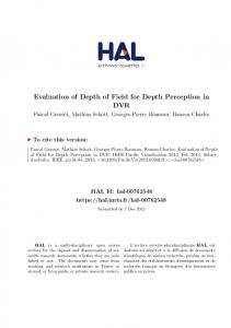
3.5 Limitations While each pixel can have a different focus and aperture setting, it is nontrivial to use compositing to achieve multiple focus depths within a single pixel. Fortunately, most pixels only contain one or two objects, so this limitation is minor, and quality remains high (Figure 3). However, when blur is very large, objects can get blurred across a vast region. For scenarios with large blur and multiple focus planes, the user would be better off using nonlinear distributed ray tracing or simulated heat diffusion, instead of compositing. 4.4 Simulated Heat Diffusion Simulated heat diffusion has of course received a great deal of attention 4 Method 3: Simulated Heat Diffusion in mathematics and mechanical engineering. The par4.1 Introduction Our diffusion method proceeds by tial differential equations that govern heat flow can, for first rendering the scene into a set of layers, which need example, be solved by complex finite element methods not be planar (Figure 5(a)). The 3D world coordinates with high-order basis functions and adaptive meshes. of each pixel are stored in a position map associated Fortunately, our domain is simply a regular image grid, with the layers. The position map is used to connect allowing simple solutions based on finite differences. We the user-specified 3D blur field to the layers (Figure find that strict physical accuracy is unnecessary, so we 5(b)). We then use the blur values associated with each use the simplest implementation available: repeated 3x3 layer to blur the layers (Figure 5(c)). Finally, the layers averaging. One complication is that conductivity valare composited from back to front using alpha blending ues are needed beyond the boundaries of an object, to [11]. One difficulty is that naive spatially varying blur properly simulate the fact that a blurred object appears produces artifacts in the form of holes appearing in the larger than an in-focus object. Figure 7 illustrates this middle of objects. However, simulated heat diffusion extrapolation Left: An object. Right: The blur map is a form of blurring that avoids these artifacts. We for that object. Center and background: We smoothly therefore blur our layers using a simple iterative imple- extrapolate the blur field to the surrounding area. mentation of diffusion in a non-homogeneous medium 4.5 Limitations and Future Work For all of its [10]. See Figure 5 for an example. advantages, simulated heat diffusion has the limita4.2 The Blur Field The user controls our heat tion that its impulse response, or point spread function diffusion method by specifying a blur field, i.e. a scalar (PSF) is essentially Gaussian. Photographers will recfield whose domain is the space of the 3D scene (R3 ) ognize that Gaussians leads to a relatively bland bokeh. and whose range is a real number specifying how much That is, the out-of-focus regions will look smooth, lackto blur. The blur field is sufficiently flexible to enable ing the circular or polygonal highlights found in real selective blurring of distracting elements, no matter how photographs. Generalized depth of field would be even those elements are distributed throughout the scene. more flexible if the user could control the PSF, as well as Specifying a blur field may be easier than designing the amount of blur. The PSF of ordinary cameras can nonlinear rays, and is more flexible than the near and be generalized to achieve non-traditional bokeh simply by placing cardboard cut-out masks on the lens. Such far surfaces of our compositing method. a mask could easily be simulated with nonlinear dis4.3 Partial Occlusion and Holes Partial occlu- tributed ray tracing, but not with heat diffusion. For sion, i.e. the fact that edges of blurred foreground ob- future work, the blur field and layered aspects of our jects appear transparent, is easily simulated as part of heat diffusion method could be used with a different the layered blur process. Opaque pixels with alpha of image filter. The challenge is in finding a filter that re1 blend with transparent pixels with alpha of 0, lead- spects visibility like heat diffusion, but provides control ing to semi-transparent regions. Traditional image fil- over the PSF. ters based on gathering or spreading can simulate partial occlusion reasonably well for realistic depth of field. 5 Future Work: A Fourth Approach However, generalized depth of field can lead to scenar- As general as the methods presented in this paper are, ios such as Figure 6, where blurred interiors can ap- further generality in blur could be achieved through a
45
Copyright © by SIAM. Unauthorized reproduction of this article is prohibited.
form of 2D vibrational motion blur. First, consider that objects could be made to appear precisely as if they were out of focus, if they were instead moving within an image-aligned disc during the exposure. Now consider that the objects could instead move in arbitrary ways, deviating from the appearance of traditional depth of field. For example, objects could move in depth, rather than merely in an image-aligned disk. This would lead to a unique type of blur. A major advantage of the motion blur approach is that, unlike compositing or heat diffusion, motion blur has a direct physical meaning. We can be assured, for example, that no holes will appear in the middle of blurred objects unless the motion happens to tear a hole in the object. To describe the motion, it should be sufficient to provide a field of generalized PSFs over the 3D scene. A generalized PSF would be a function whose domain is the 2D “aperture”, and whose value is a 3D displacement vector indicating where the motion takes a point. Rendering would simply involve sampling the “aperture”, which means warping the 3D scene based on the generalized PSF field. Partial occlusion will happen naturally, as some samples will contain occlusions, but other samples will not. 6 Conclusion As useful as depth of field is to photographers, we have shown that more flexible depth of field is possible via computer graphics. We have shown that depth of field can be generalized in at least three useful ways. Each of our methods is ideal for different use cases. Situations demanding simplicity and speed should use compositing. Situations demanding the highest possible image quality should use nonlinear ray tracing. Finally, situations demanding complete flexibility should use simulated heat diffusion. Perhaps other generalizations exist as well, and we challenge the reader to consider in what other useful ways can depth of field be extended. References [1] B. A. Barsky, D. R. Horn, S. A. Klein, J. A. Pang, and M. Yuf, Camera models and optical systems used in computer graphics: Part i, image based techniques., in Proceedings of the 2003 International Conference on Computational Science and its Applications (ICCSA’03), 2003, pp. 246–255. [2] B. A. Barsky, D. R. Horn, S. A. Klein, J. A. Pang, and M. Yuf, Camera models and optical systems used in computer graphics: Part ii, image based techniques., in Proceedings of the 2003 International Conference on Computational Science and its Applications (ICCSA’03), 2003, pp. 256–265.
46
[3] M. Bertalmio and P. Fort and D. SanchezCrespo (2004) Real-time, accurate depth of field using anisotropic diffusion and programmable graphics cards. 3DPT 04: Proceedings of the 3D Data Processing, Visualization, and Transmission, 2nd International Symposium. 767–77, IEEE Computer Society. [4] R.L. Cook, T. Porter and L. Carpenter 1984. Distributed ray tracing. SIGGRAPH Comput. Graph. 18, 3 (Jul. 1984), 137-145. DOI= http://doi.acm.org/10.1145/964965.808590 [5] J. Demers, GPU Gems, Addison Wesley, 2004, pp. 375–390. [6] P. Haeberli and K. Akeley (1990) The accumulation buffer: hardware support for high-quality rendering, In SIGGRAPH ’90: Proceedings of the 17th annual conference on Computer Graphics and interactive techniques, Dallas, TX, USA, pp. 309–318. [7] M. Kass, A. Lefohn, D. Owens (2006) Interactive depth of field using simulated diffusion on a GPU. Pixar Animation Studios Tech Report. [8] R. Kosara, S. Miksch and H. Hauser (2001) Semantic depth of field. Proceedings of the 2001 IEEE Symposium on Information Visualization (InfoVis 2001), pp. 97-104, IEEE Computer Society Press. [9] T. Kosloff, M. Tao, and B. Barsky, Depth of field postprocessing for layered scenes using constant-time rectangle spreading, in GI ’09: Proceedings of Graphics Interface 2009, pp. 39–46. [10] T.J. Kosloff and B.A. Barsky (2007) An algorithm for rendering generalized depth of field effects Based on Simulated Heat Diffusion, In Proceedings of the 2007 International Conference on Computational Science and Its Applications (ICCSA 2007), Kuala Lumpur, 26-29 August 2007. Seventh International Workshop on Computational Geometry and Applications (CGA’07) Springer-Verlag Lecture Notes in Computer Science (LNCS), Berlin/Heidelberg, pp. 1124-1140 (Invited paper). [11] T. Porter and T. Duff, Compositing digital images In SIGGRAPH Comput. Graph. 18, 3 (Jul. 1984), pp. 253–259 [12] M. Potmesil and I. Chakravarty, Synthetic image generation with a lens and aperture camera model, in ACM Transactions on Graphics 1(2), 1982, pp. 85– 108. [13] T. Scheuermann and N. Tatarchuk, Advanced depth of field rendering, in ShaderX3: Advanced Rendering with DirectX and OpenGL, 2004. [14] C. Scofield, 2 1/2-d depth of field simulation for computer animation, in Graphics Gems III, Morgan Kaufmann, 1994. [15] M. Shinya, Post-filtering for depth of field simulation with ray distribution buffer, in Proceedings of Graphics Interface ’94, Canadian Information Processing Society, 1994, pp. 59–66. [16] A. Veeraraghavan, R. Raskar, A. Agrawal, A. Mohan and J. Tumblin, Dappled photography: mask enhanced cameras for heterodyned light fields in
Copyright © by SIAM. Unauthorized reproduction of this article is prohibited.
SIGGRAPH 2007, (Jul. 2007), pp. 69. [17] T. Zhou, J. X. Chen, and M. Pullen, Accurate depth of field simulation in real time, in Computer Graphics Forum 26(1), 2007, pp. 15–23.
Figure 2: An image synthesized with our nonlinear distributed ray tracing technique.
Figure 4: Near and far focal surfaces for the compoiting technique.
(a) Input: Everything in perfect focus.
(b) A blur map.
Figure 3: An image synthesized with our compositing technique. (c) Image blurred using diffusion, with the blur map acting as a conductivity map.
Figure 5: Generalized depth of field via simulated heat diffusion
47
Copyright © by SIAM. Unauthorized reproduction of this article is prohibited.
Figure 6: A blurred rectangular region with traditional image filters (left) and simulated heat diffusion(right)
Figure 7: Simulated heat diffusion requires that we extrapolate blur values beyond the boundaries of the object.
48
Copyright © by SIAM. Unauthorized reproduction of this article is prohibited.