Visual Servoing For A Scale Model Autonomous Helicopter

Proceedings of the 2001 IEEE International Conference on Robotics & Automation Seoul, Korea • May 21-26, 2001

Visual Servoing For A Scale Model Autonomous Helicopter A. CHRIETTEy , T. HAMEL y CEMIF Universite d'Evry. 40 rue du Pelvoux, Evry, France.

Abstract{A control design to stabilise a reduced scale autonomous helicopter equipped with a camera is presented. The proposed algorithm is motivated by recent work in image-based visual servoing control for under-actuated dynamic systems. This work is extended by considering models that contain weakly nonminimum phase zero dynamics. This is an important class of systems since an oset between the camera and the centre of mass for a typical 'dynamic' autonomous vehicle will result in zero dynamics occurring in the image dynamics. In this paper we propose a simpli ed model of dynamics of the helicopter and show that by placing some constraints in the choice of the position of the camera we can minimise the eect of the zero dynamics.

1

Introduction

Unmanned Air Vehicles (UAVs) are becoming an exciting new application area for modern non-linear control theory. Several authors in this last decade have contributed to the study and development of dynamics models which are dedicated to the UAV [10, 4]. Their small size, highly coupled dynamics and low cost implementation provide an ideal testing ground for sophisticated control techniques. One major problem that arises in the control of such vehicles is the diÆculty of measuring non-inertial variables such as position, orientation and velocity. Acceleration and angular velocity may be measured using accelerations and rate gyros. To overcome the problem of regulating the position of a UAV without expensive ground based systems, a number of authors have considered using visual feedback. This kind of control is expressed by `Visual Servoing'. Early implementations of visual servoing algorithms were used to position a robotic manipulator relative to a xed visual target [1]. More recently, visual servoing has been proposed for applications in mobile robotics, for example in the control of a car-like vehicle [9, 6]. In all approaches feedback control is used to regulate an error function measured directly in the task space and derived from the control objective. This approach does not generalise well to the case where the dynamics of the system are important. Most existing applications exploit a high gain or feedback linearization (computed torque) design to reduce the system to a controllable kinematic model, for which the image-based 0-7803-6475-9/01/$10.00 © 2001 IEEE

y

and R. MAHONYz

z Dep. of Elec. and Comp. Sys. Eng. Monash University, Clayton, Victoria, 3800, Australia.

visual servoing techniques were developed [3]. Recently Hamel and Mahony [2] presented a novel new algorithm for visual servoing of an under-actuated dynamic rigid body system based on exploiting the passivity-like properties of rigid body motion. In this paper we consider a similar problem to that solved in [2]. However, the model considered is extended to incorporate the possibility of zero dynamics in the system resulting from an oset between the camera and the centre of mass of the UAV. In practice, this eect is unavoidable and, since the zero dynamics of a Hamiltonian system are Hamiltonian, may result in small non-decaying oscillations in the motion of the UAV. An idealized model of an autonomous model helicopter is considered as a base for the theoretical development undertaken. The principal contribution of the paper is to show that by choosing a suitable position for the camera, it is possible to limit the eects of the zero dynamics. The paper is divided into ve sections including the present overview. In Section 2 an idealised model of an autonomous helicopter is presented based on the Newton-Euler equations. In section 3 the image dynamics are derived. Section 4 shows how to derive the proposed control law using a robust backstepping techniques. Finally, in the section 5, we give some simulations and results. 2

Helicopter Model

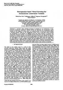
In this section a dynamic model of autonomous helicopter equipped with a camera is proposed. The model is derived from Newton-Euler equations by assuming that the helicopter body is rigid. For details of the dynamic equations, please refer to [4] or [7]. Denote the body airframe by letter A. let I = fEx ; Ey ; Ez g denote a right-hand inertial frame stationary with respect to the earth. Let the vectors  = (x; y; z )T and c = (xc ; yc; zc)T denote respectively the position of the centre of mass of the helicopter and the focal point of the camera relative to the frame I : Let A = fE1a; E2a ; E3a g be a (right-hand) body xed frame for A, and C = fE1c ; E2c ; E3cg denote the camera xed frame of the camera, (see g. 1). In addition, let R 2 SO(3) be an orthogonal rotation matrix which give the orientation of the helicopter relative to the inertial frame R : A ! I . The orientation of the camera relative to the body xed frame of 1701

the helicopter is given by a xed rotation Rc : C ! A.

Figure 1: Components of lift forces and osets. In the present paper, it is preferable to work directly with the force inputs decomposed into orthogonal components and assume that each of these inputs is an independent control. As shown on gure (1), the main rotor lift is decomposed into three components ( w2 ; w1 ; u) 2 A orientated in the directions fE1a ; E2a ; E3a g. Furthermore, the force due the tail rotor is always oriented in the second axis direction E2a and is written (0; w3 ; 0) 2 A. As shown in [8], by applying Newton's equations of motions, the dynamics of an autonomous helicopter are _ = v (1) 2 1 3 mv_ = uRe3 + mge3 w Re1 + (w w )Re2 (2) _R = Rsk( ) (3) 3 1 3 3 3 2 _ I =

 I + (lM w lT w )e1 + lM w e2 + 1 3 lT w e3 + QM e3 + QT e2 : (4) In the above dynamics, the two torque controls governing roll and pitch, Eq.(2), generate sideways forces on the airframe which introduce zero dynamics into the system. Theses forces are known as small body forces. In this
model, it is assumed that lM = 0; 0; lM3
2 A, where lM3 > 0 and lT = lT1 ; 0; lT3 : 3

A Reduced Model

In this paper, it is proposed to nd the optimal position for the camera that will reduced the eects of the small body forces. Assuming that the inertia matrix I is diagonal, then Eq.(4) may be rewritten explicitly as follows: _ 1 = 3 2 (I3 I2 ) + (lM3 w1 lT3 w3 ); (5) I1

_ 2 = 3 1 (I1 I3 ) + QT + lM3 w2 ; (6) I2

_ 3 = 2 1 (I2 I1 ) + QM + lT1 w3 : (7) I3

It is assumed that the anti-torque associated with the rotor air resistance is known and dierentiable. The control input w is decomposed into two parts w = w~0 + w~ where w~0 is the component of the torque input that counter-acts air resistance of the rotors and w~ is the part that contributes directly to the control of the helicopter. To counter-act the anti-torque QM e3 due to the main rotor, choose w~03 = Ql1TM . Let (I2 I1 ) = ". Thus, one has _ 3 = 2 1 " + lT1 w~3 I3

Assume that 3 (0) = 0 (otherwise initially stabilise the yaw before commencing the control design) then by choosing

" (8) w~3 = 2 1 1 lT one ensures that 3  0 for all time. Choosing w~02 = Ql3MT , cancels the eect of the antitorque QT (t). It is also necessary to cancel the contri-

bution to the rst component torque due to the input w~03 and non-zero oset lT3 . Set l3 l3 w~01 = 3T w03 = 1 T3 QM ; lM lT lM

(9)

Based on the above choices, the equation of motion Eqn's 2-4 may be written in a reduced form : mv_ = uRe3 w~2 Re1 + (w~1 w~3 )Re2 (10)   3 3 QT lM lT + mge3 + l3 l1 QM Re2 + l3 Re1 M T M _ = (lM3 w~1 lT3 w~3 )e1 + lM3 w~2 e2: I

(11)

The inputs for this system are u, w~1 and w~2 . In addition, the control input w~3 is used to stabilize 3 (t) at 0. All the terms in Eq. (10) directly independent of the control input are written separately in brackets. These terms form the disturbance to the translation dynamics, dominate by the gravitational force mg, but also depending on the rotation matrix R as well as the rotor drag terms. A consequence of the perturbation terms in Eq.(10) is that the stationary point of the dynamics Eqn's (1,10, 3 and 11) corresponding to the helicopter hovering requires a non-trivial rotation R. Indeed, in stationary ight any helicopter must y with slight permanent inclination of the principal lift force uRe3 to compensate for the small body force resulting from the torque control necessary to cancel rotor drag. It is important for control design in visual servoing to represent the dynamics of the helicopter in the camera xed frame. Let vc be the velocity of focal point of the camera relative to the inertial frame, and let Vc its representation in the camera xed frame. 1702

Let d 2 R3 be a translation vector between (A) and (C ), one has c =  + Rd (12) Considering only a displacement in the E3a axis, that is d = d3 e3 = (0; 0; d3 )T , the rotational matrix Rc = I3 , the full linear dynamics of a helicopter expressed in the camera xed frame are given by _c = RVc; (13) _ mVc = m  (Vc  d) ue3 (14)   3 3 +mgRT e3 + lMl3 l1lT QM e2 + Ql3T e1 M T

0

M

3 3 w~2 w~2 + m dI2 lM 3 3 w~1 l3 w~3
w~3 ) m dI1 lM T

+B @ (w ~1

1 C A

0 From this equation it is clear that the displacement d3 may be chosen such that the rst entries of the right hand side of Eq.(15) are independent of the control action w~2 . Set: d3 =

I2 3 mlM

(15)

In order, to cancel the centrifugal forces  (  d) introduced by the oset of the point c , de ne the following modi ed control u
u = u + md3 ( 1 )2 + ( 2 )2 (16) By this choice and using Eq.(15), the reduced linear model dynamics may be written : _c = RVc ; (17) T _ mVc = msk( )c Vc ue3 + mgR e3 +   l3 I l3 I X + "w~1 + T 2 3 M 1 w~3 e2 (18) I l 



1M

where X = lMl3M l1TlT QM e2 + Ql3MT e1 and we assume  that the control algorithm has access to X_ and X: In Eq.(18), the presence of the small body forces, which couple torque inputs to the translational dynamics are only present in the second axis direction E2a . The zero dynamics are generated by the additional control inputs w~1 and w~3 that are not exactly cancelled by the choice of camera position. In practice, the presence of the small body forces destroys the design of a robust control, in particular the backstepping procedure which use to give our control design. In the present paper and as proposed in [8, 4], to avoid this problem, we ignore the control terms contributing to the zero dynamics eect. Furthermore, as proposed in [8], we can give an analysis which shows that as long as the small body forces are suÆciently small the proposed control design in this paper will ensure the same properties for the full system. 3

3

4

Image Dynamics

Let a set of n points Pi0 of a xed target, relative to the inertial frame (I ) and observed from the camera, and Let Pi the representation of Pi0 in the camera xed frame, then Pi is given by Pi = RT (Pi0 c ) A backstepping control design has passivity-like properties from virtual input to the backstepping error [5]. In a recent paper [2] it was shown that these structural passivity-like properties are present in the image space dynamics if and only if the spherical projection of an observed point is used. Denoting the spherical projection of an image point Pi by pi the image dynamics are given by (see [2] for more details) V p_i = sk( )c pi + p i r i

(19)

Here ri = jPi j and Vi 2 C is the observed velocity of the target point represented in the body xed frame of the camera. The matrix p = (I3 pi pTi ) is the projection onto the tangent space of the spherical image surface at the point pi . If the inertial velocity of the target point Pi0 is equal to zero then Vi = Vc , where Vc is the velocity of the camera relative to the camera xed frame. Thus Eq. (19) becomes: p_i =  pi

pi V ri c

Here the focal length of the spherical camera has been normalized to unity and it is assumed that the target points are stationary in the inertial frame. We wish to stablize the camera to a desired pose (position and orientation) with respect to a target of interest. Let pi denote the desired visual features, xed relative to the inertial frame. The image based error vector chosen is Æ = vect(pi pi ) 2 R3n Let 0 1 T 1 r1 (I3 p1 p1 ) C .. =B @ A: . 1 (I3 pn pT ) n rn Computing the rst order dynamics of Æ, it yields Æ_ = diag(sk( ))Æ Vc : A common approach taken in image based visual servoing is to average the available visual information contained in the full error Æ. This is achieved by introducing a combination matrix C that `codes' the averaging process and de ning a reduced error Ær = CÆ; C 2 R33n (20) 1703

Following the approach of Hamel and Mahony [2], the reduced error is only three dimensional and it is impossible to derive full pose information from the reduced error. However, the reduced error does suf ce to fully specify UAVs position and yields passivelike behaviour suitable for application of backstepping control design as long as the matrix C satis es C  = Q > 0 and C diag( sk( )) = sk( )C; 8 2 R3 A matrix respecting these conditions will be of the form C = [ 1 I


n I ]; i  0; i = 1; :::; n. Note that the property C  = Q > 0 relies on the fact that ri > 0. The reduced error vector considered is Æ1 = C Æ and the full dynamics of Æ1 are given by Æ_1 = sk( )Æ1 Q Vc : (21) The exact value of Q is unknown, however, it is possible to obtain bounds on the eigenvalues of Q from upper and lower bounds on distance of the UAV to the target [2] and these are used in the control design. 5

Visual servoing for helicopter

In this section, a control design robust backstepping techniques [5] is proposed for visual servoing of the idealised autonomous helicopter dynamics proposed earlier. From Eq.(21) and the reduced rigid body dynamics Eqn's (18, 3 and 11), the full dynamics of the error Æ1 may be written: Æ_1 = sk( ):Æ1 Q Vc (22) T mV_c = m  Vc ue3 + mgR e3 + X (23) R_ = Rsk( ) (24) 3 1 3 3 3 2 _ I

= (lM w~ lT w~ )e1 + lM w~ e2 (25) De ne the rst storage function S1 by: 1 S1 = jÆ1 j2 2 Deriving S1 and recalling Eq. (22) yields: S_ 1 = Æ1T Q Vc

(26)

If the velocity Vc were available as a control input, then the choice of Vc = Æ is suÆcient to stabilise S1 . Thus the virtual control chosen for this step is k Vcv = 1 Æ1 m

(27)

where k1 is a positive constant. Since the matrix Q is positive de nite and if Vcv  Vc then S_ 1 = k1 Æ T Q Æ is negative de nite in Æ . Thus, Eq.(22) 1 m 1  1 becomes k k1 Q Æ1 1 Q Æ2 ; (28) Æ_1 = sk( )Æ1 m

m

where Æ2 is a new error term given by Æ2 =

m V Æ; k1 c 1

(29)

the dierence between the true and the desired velocity. The derivative of S1 may be written k S_ 1 = 1 Æ1T Q Æ1 m

k1 T Æ Q Æ m 1 2

(30)

The second storage function considered is 1 S2 = S1 + jÆ2 j2 2 Taking the derivative of S2 and substituting for Eq. (23), yields k k1 T Æ1 Q Æ1 + 1 Æ2T Q Æ2 m m 1 T + k Æ2 ( ue3 + mgRT e3 + X ) (31) 1 Let ( ue3 + mgRT e3 )v the virtual2 control chosen for this step ( ue3 + mgRT e3 )v = k1mk2 Æ2 X . With this choice the derivative of Æ2 is given by k k kk Æ_2 = sk( )Æ2 + 1 Q Æ1 1 (k2 I3 Q )Æ2 + 1 2 Æ3 m m m where Æ3 represents the third error term   k12 k2 m T ( ue3 + mgR e3 ) + m Æ2 + X Æ3 = 2 k1 k2 S_ 2 =

(32) In the formal process of backstepping the new error Æ3 would now be dierentiated. This requires a formal time derivative of the input u. To provide this the input u is dynamically extended u = u~ (33) The motivation for adding a double integrator here is to ensure that the relative degree of the new input u~ with respect to the position co-ordinates c is the same as the relative degree of w~1 , w~2 and w~3 with respect to the position. In the present derivation, all inputs are chosen to have relative degree four with respect to the position c . The derivative of the second storage function is: S_ 2 =

k1 T Æ Q Æ m 1 1

k1 T Æ (k I m 2 23

kk Q )Æ2 + 1 2 Æ2T Æ3 m

(34) where k2 is chosen such that k2 > max (Q ). The backstepping process continued by taking the derivative of Æ3 k kk k Æ_3 = sk( )Æ3 + 1 Q Æ1 1 (k2 I3 Q )Æ2 + 1 2 Æ3 m m m m _ m _ + 2 X 2 (ue3 + sk( c )(ue3 X )) k1 k2

1704

k1 k2

The last storage function in the backstepping procedure is the Lyapunov candidate function 1 S4 = S3 + jÆ4 j2 2 Deriving S4 and recalling Eq.(38) one obtains

The virtual control chosen in this step is 2 3 + k2 k1 ) Æ + X: (u_ e3 + sk( )(ue3 X ))v = k1 k2 (km 3 _ 2

Using this choice yields Æ_3 =

sk( )Æ3 + km1 Q Æ1 k1 (k I m 23

Q )Æ2

k3 Æ m 3

(35) (k3 + k2 k1 ) Æ : m

k k1 T k3 T S_ 4 = 1 Æ1T Q Æ1 Æ2 (k2 I3 Q)Æ2 Æ Æ m m m 3 3 + km1 Æ4T (k2 I3 Q )Æ2 + km1 Æ3T Q Æ1 + km1 Æ3T Q Æ2 k4 T k1 T Æ4 Æ4 Æ Q Æ m m 4 1

4

Here Æ4 is the nal error term introduced in the design procedure m2 (u_ e3 + sk( )(ue3 X ) X_ ) Æ4 = Æ3 (36) k12 k2 (k3 + k2 k1 ) Let S3 be a storage function associated with this step of the procedure 1 S3 = S2 + jÆ3 j2 (37) 2 Deriving S3 and recalling Eq. (34) one obtains k1 T k k1 T Æ Q Æ Æ (k I Q )Æ2 + 1 Æ3T Q Æ1 m 1 1 m 2 23 m k1 T ( k3 + k2 k1 ) T k3 T + m Æ3 Q Æ2 Æ3 Æ4 Æ Æ (38) m m 3 3 The derivative of Æ4 is

S_ 3 =

k k1 Q Æ1 + 1 (k2 I3 Q )Æ2 Æ_4 = sk( )Æ3 m m k3 ( k3 + k2 k1 ) m2 + m Æ3 + Æ4 X 2 m k1 k2 (k3 + k2 k1 )   2 _ ue3 X ) + k2 k (km+ k k ) ue3 + sk( )( 1 2 3 2 1 2 + k2 k (km+ k k ) sk( )(u_ e3 X_ ) 1 2 3 2 1

Proposition [2] Consider the dynamics given by Eqn's (22-25). Let the vector controller given by Eq.(39) and recover the original inputs from Eq.(41). Then the main objective Æ1 converges to zero if the control gains satisfy the following constraints :

k1 > 0 k2 > max (Q )

At this stage the actual control inputs enter into the equations through u = u~ and _ via Eq. (25). The nal stage of the backstepping process is choose a control input. The following vector equation is solved for the control inputs u and w~.   u~e3 + _ c  ( ue3 + X ) = sk( c)( u_ e3 + X_ ) k2 k1 + k3 + k4 k2 k (k + k k ) Æ X + 1 2 3 2 1 ( sk( )Æ m2

c 3

+ k2mk1 Æ3 )

m



 1 1 k3 > k1 max (Q ) + min (Q ) k2 min(Q )   max (Q ) k2 min (Q k4 > k1 +  (Q ) k  (Q )

min 

2

max



where min (Q ) and max (Q ) represent the lower and upper bounds of Q .

4

(39)

Given the above choice the dynamics of Æ4 becomes k (k k + k ) k1 Q Æ + 1 (k I Q )Æ2 + 2 1 3 Æ3 Æ_4 = m 1 m 23 m k4 Æ m 4

Recall that the dynamics of the angular velocity of the camera expressed in the body xed frame are given by Eq. (11). Expanding the vector cross product and collecting terms then the left hand side of Eq. (39) may be written as: 0 1 3 w~2 u lM I 2 B C l3M w~1 l3T w~3 u (41) @ A I1 3 3 l w ~ ~ 1 lT w 3 T w ~ 3 T 2 M u~ lM I2 e1 X + e2 X I1 Thus, as long as u 6= 0 there is a unique control input (~u; w~1 ; w~2 ; w~3 ) that solves Eq. (39). In hover conditions, the condition u 6= 0 will always hold since u corresponds to the heave force used to compensate gravitational acceleration. A second interesting observation is that the presence of the drag terms X introduce parasitic terms sk( )X which are cancelled by the input u~. Finally, as indicated in the subsection 2.1, the control design is complete when the the third input w~3 free to x 3 at zero.

(40)

The proof of this proposition is a direct application of the principals of the backstepping based on the development leading up the proposition statement. 6 Simulation and results

In this section we present a simulation with the aim to validate the proposed control design. The task considered is to position a camera relative to the planar square target. The target is modelled by four

1705

points on the vertices of the square. Naturally for this task, the signals available are the pixel co-ordinates of the four points observed by the camera, denoted f(u1 ; v1 ); (u2 ; v2 ); (u3 ; v3 ); (u4 ; v4 )g. The simulated spherical co-ordinates (xi ; yi ; zi ) of the four points are respectively given by xi = pfu2i+v2 , yi = pfv2i+v2 and i i p zi = f 2 u2i vi2 . For more details the reader is referred to [2]. The desired image feature are chosen such that the camera is located several meters above the square. It is de ned by : f( a; a); (a; a); (a; a); ( a; a)g where a represents the ratio between thevertex length and the nal desired range. In this simulation the parameter a has been chosen equal to 0.4851 corresponding to a location of six meters of the camera above the target. The magnitude of the initial force input is chosen to be u0 = gm  177 corresponding to the fact that the helicopter is initially in hover ight. The initial position is:
0 = 5 4 16 T ; _0 = 0 and 0 = _ 0 = 0: The center of the target ^ is chosen to be :
^0 = 0 0 6 T the choice of the values of min (Q ) and max (Q ) depends respectively on initial conditions and the desired location, it follows that : min(Q ) = 0:0206 and max (Q ) = 0:3686: From the above choice, we have used the following control gains: k1 = 0:2; k2 = 1; k3 = 3; k4 = 3, that satis es conditions given in Proposition. Simulations results of the helicopter system control algorithm are given on gures 2 and 3.

−1

−0.8

−0.6

−0.4

−0.2

0

0.2

0.4

0.6

0.8

1

[2] [3] [4] [5] [6] [7]

14 12

z

10 8 6 4 2

[8]

0 6 6

2

4 0

2 0

−2

−2

−4 y

−4 −6

−6

x

[9]

Figure 2: Positioning of the helicopter with respect to the target. References

[1]

Espiau, B., Chaumette, F., Rives, B., \A new approach to visual servoing in Robotics", IEEE Transactions on Robotics and Automation, 8, 3 (1992), pp. 313-326.

0.8

0.6

0.4

0.2

0

−0.2

−0.4

−0.6

−0.8

−1

Figure 3: Evolution of the image features in the image plan.

16

4

1

[10]

1706

Hamel, T., Mahony, R., \Visual servoing of underactuated dynamic rigid body system : An image space approach", In Proceedings of the 39th Conference on Decision and Control, 2000. Hutchinson, S., Hager, G., Cork, P., \A tutorial on servo control". IEEE Transactions on Robotics and Automation, 12, 5, (1996), pp. 759-766. Koo, J.T., Sastry, S., \Output tracking control design of a helicopter model based on approximate linearization", In Proceedings of the 37th Conference on Decision and Control, Florida, December 1998. Krstic, M., Kanellakopoulos, I., Kokotoviv, P.V, \Nonlinear and adaptive control design", American Mathematical Society, Rhode Islande, USA, 1995. Ma, Yi., Kosecka, J., Sastry, S., \Vision guided navigation for a nonholonomic mobile robot", IEEE Transactions on Robotics and Automation, june (1999). Mahony, R., Hamel, T., Dzul, A., \Hover control via approximate Lyapunov control for a model helicopter", In Proceedings of the 1999 Conference on Decision and Control, Phoenix, Arizona, U.S.A, 1999. Mahony, R., Lozano, R., \Exact Tracking Control for an Autonomous Helicopter in Hover-like Manouvers", International Conference on Robotics and Automation, 1999. Pissard, G., Rives, P., \Applying visuel servoing to control of a mobile hand-eye system", In Proceedings of the International Conference on Robotics and Automation, Nagasaki, JAPAN, 1995. Shaufelberger, W., Geering, H., \Case study on helicopter control", Invited session in Control of Complex Systems, (COSY), October 1998.