On the Use of State Predictors in Networked Control Systems

Author manuscript, published in "N/P"

1 On the Use of State Predictors in Networked Control Systems E. Witrant, D. Georges, C. Canudas-de-Wit, and M. Alamir

hal-00196856, version 1 - 13 Dec 2007

Laboratoire d’Automatique de Grenoble, ENSIEG, B.P. 46, 38 402 Saint Martin d’H`eres, FRANCE witrant, georges, ccanudas, alamir @lag.ensieg.inpg.fr Summary. Without pretending to be exhaustive, the aim of this chapter is to give an overview on the use of the state predictor in the context of time-delay systems, and more particularly for the stabilisation of networked control systems. We show that the stabilisation of a system through a deterministic network can be considered as the stabilisation of a time-delayed system with a delay of known dynamics. The predictor approach is proposed, along with some historical background on its application to time-delayed systems, to solve this problem. Some simulation results are also presented. Key words: Networked controlled systems, predictive control, time-delay systems.

1.1 Introduction The networked control systems (NCS) constitute a particular class of control problems, where the communication channel influence is crucial in the stabilisation of the remote system and cannot be neglected. The control setup is shown in Figure (1.1), where the system considered can be open-loop unstable. The sensor, actuator and system are remotely commissioned by a controller that interchange measurements and control signals through a communication network. This network is used by multiple systems and a packet management law (router, switch, priority level . . .) is introduced to distribute the information. A Transfer Protocol (TP) is implemented to allow users to send and receive data over the network. The impact of such network is to introduce a time-varying delay in the data transmission between the system and the controller, due to the multiple users interaction. The time-varying delay makes the problem more difficult since the timetranslation is not reversible and the results established in the frequency domain cannot be used (like the Smith predictor [1]). Most of the existing control methods (like the Lyapunov-Krasovskii approaches) result in a LMI formulation based on a constant time-delay, or a known upper bound on it (see for

2

E. Witrant, D. Georges, C. Canudas-de-Wit, and M. Alamir

hal-00196856, version 1 - 13 Dec 2007

Fig. 1.1. Closed-loop network controlled system.

example [2] or [3]). The case of time-varying or state-dependent delays can be treated along with the solutions presented in [4], and [5] as long as the system is open-loop stable. These solutions do not allow for a direct use of the time-delay dynamics in the design of the control law and naturally yield to conservative results. The state predictor approach is particularly efficient to stabilize a delayed (possibly open-loop unstable) system since it results in the pole placement (finite spectrum assignment) of the closed-loop system. It can be applied to the case of time-varying delays by considering a predictor with a time-varying horizon, thus explicitly including the dynamics of a deterministic network in the control synthesis. This chapter is organized as follows. The first part details the specificities introduced by the use of a deterministic network in the communication channel, along with the characteristics of the induced time delay and a description of the controlled system. The second section presents some historical key points on the use of the state predictors to assign a finite spectrum to time-delayed systems. In the third section, the state predictor is combined with some other control and analysis tools in order to design a robust control scheme, possibly with an explicit use of the network dynamics or based on a state observer. Some issues on the related numerical problems are also considered and an application example is finally proposed.

1.2 Problem statement: control through TP networks The networked controlled systems are characterized by some specific transmission protocol dynamics that can be explicitly used in the design of the control feedback. This dynamics induces a time-varing delay which depends on the interaction of multiple users on the network. A transfer protocol is set between the emitters and the network to manage the exchange of packets (emission and reception). The TP determines the emitter’s window size and manage the reception of packets. Considering the

1 On the Use of State Predictors in Networked Control Systems

3

class of secure networks we can guarantee that there is no loss of information in the communication process (all the lost packets are re-emitted), which results in a bounded transmission delay. Examples of such protocols (a detailed description can be found in [6]) are the Transfer Control Protocol (TCP) and Sequenced Packet Exchange (SPX) schemes. An other example is a dedicated network used to control a supply chain or an embedded system; in that case, the TP can be freely designed to ensure the desired properties. The delay induced by the network is then the delay experienced by the control and measurement signals. Therefore, the lossless property of the network ensures that the delays are bounded and cannot increase as fast as the time (since it is the delay measured from the system or the control law sites). This motivates the following property. H1) The time-delay τ (t) induced by the communication network satisfies, for all t ≥ 0, 0 ≤ τ (t) ≤ τmax

and

τ˙ (t) < 1,

hal-00196856, version 1 - 13 Dec 2007

where τmax ≥ 0 is an upper bound on the delay. Note that this hypothesis is generally used to ensure the stability or the controllability of time-delay systems. The time-delay dynamics induced by a TP network can be described in a continuous, discrete or hybrid framework. For analysis purposes, we chose the continuous formulation but the proposed results can easily be extended to the other kinds of models. The induced delay is then described by the general class of systems that write as z(t) ˙ = f (z(t), ud (t)), τ (t) = h(z(t), ud (t)),

z(0) = z0 ,

(1.1) (1.2)

where •

z(t) is the internal state of the network (with initial state z0 ) , that describes the time evolution of the emitters window size Wi (t) (for i = 1 . . . N sources connected to the network) and the router’s queue length q(t), for example. In that case, the state writes as z(t) = [W1 (t) . . . WN (t) q(t)]T , • ud (t) is the exogenous input to the system, which is the number of users N (t) and the link capacity C(t), if both are time-varying. We then have ud (t) = {N (t), C(t)}, • f (z(t), ud (t)) describes the internal dynamics of the network, set by the TP on the window sizes and by the queue management scheme on the queue length, if a buffer is used to manage the packets, • h(z(t), ud (t)) gives the resulting delay τ (t) from the whole model. Note that (1.1)-(1.2) describes an autonomous system with an exogenous input ud (t). This input is assumed to be known over a certain range of time ahead of the present time (equal to the maximum delay expected τmax ) in order to

4

E. Witrant, D. Georges, C. Canudas-de-Wit, and M. Alamir

use the predictive approach. This would be the case for periodic systems or if the transfer protocol is set to declare to the network that its source will emit and wait during τmax before starting the emission. An appropriate robustness analysis focused on the predictor sensitivity with respect to the time-delay model can be used to remove this hypothesis. The remotely controlled system writes as: x(t) ˙ = Ax(t) + Bu(t − τ (t)), y(t) = Cx(t),

x(0) = x0 ,

(1.3) (1.4)

where x ∈ Rn is the internal state, u ∈ Rl is the control input, y ∈ Rm is the system output, and A, B, C are matrices of appropriate dimensions. The pairs (A, B) and (A, C) are assumed to be controllable and observable, respectively, but no assumption is made on the stability of A.

hal-00196856, version 1 - 13 Dec 2007

1.3 Historical Background After a short recall on the concept of commandability in the case of the systems with a delayed input, we present in this section the main results obtained in the years 1970-1980 concerning the state predictor. More precisely, the concepts of finite spectrum assignment, system reduction and the use of the predictor to stabilize systems with a delayed input if this delay is timevarying are detailed. The state is supposed to be completely known to establish the control law. 1.3.1 Controllability The controllability of linear systems with time delays in control is not trivial and was specifically studied in [7]. We consider the general class of systems described on [t0 , t1 ] by x(t) ˙ = A(t)x(t) +

k X

Bi (t)u(t − τi ),

(1.5)

i=0

where A(t), Bi (t) are bounded measurable matrices of size n × n and n × l, respectively, and 0 = τ0 < τ1 < . . . < τk are real numbers. The controllability of the complete state is usually defined as follows Definition 1. The complete state of the process (1.5) at time t is the set xc (t) = {x(t), v(t, s)}, where v(t, s) = u(s), s ∈ [t − τk , t). Definition 2. The complete state xc (t0 ) is said to be controllable on [t0 , t1 ] if there exists a control u such that x(t1 ) = 0.

1 On the Use of State Predictors in Networked Control Systems

5

Definition 3. The complete state xc (t0 ) is said to be absolutely controllable on [t0 , t1 ] if there exists a control u such that xc (t1 ) = 0 (both x(t1 ) = 0 and v(t1 , s) = 0). Definition 4. The system (1.5) is said to be (absolutely) controllable on [t0 , t1 ] if and only if every complete state is (absolutely) controllable on this interval. These definitions show the influence of the delay on the concept of state and commandability. Indeed, we do not consider an instantaneous state but an evolution on a time-dependent horizon: the control law u(·) must be known on the horizon [t − maxk τk , t] to compute the value of x(t). ˙ This comes from the fact that, if two control laws have the same value at a given instant t but a different history then the system trajectories will be different. This principle is equivalent to the one used in the definition of the dynamics of a time-delay system writing as x(t) ˙ = An x(t) + Ad x(t − τ ),

hal-00196856, version 1 - 13 Dec 2007

where a proper initial condition is expressed in [2] as x(t0 + θ) = φ(θ),

θ ∈ [−τ, 0],

ν (t0 , φ) ∈ R+ × Cn, τ

ν with Cn, τ = {φ ∈ Cn, τ : ||φ||c < ν}, where ν is a positive real number, ||φ||C = sup−τ ≤t≤0 ||φ||, || · || refers to the euclidian norm and Cn,τ = C([−τ, 0], Rn ) indicates the Banach space of the continuous vector functions projecting the interval [−τ, 0] in Rn with a uniformly convergent topology. The concept of complete state of the first definition is thus introduced to take into account the history of the control law. The previous definitions are an application of the concept of commandability, in the traditional sense, to the class of systems considered. We take into account the fact that the control law history has to be known before the system initialization (at time t0 ) and then kept in memory on the time interval [t − maxk τk , t] to ensure the uniqueness of the trajectory described by (1.5).

Remark 1. For simplicity sake, we will consider that the values of the control law preceding the system initialization are null and that their history is preserved on the necessary horizon. The initial conditions of the system are thus reduced to x(t0 ) and the traditional concepts of commandability can be applied directly. The use of the the state predictor allows, because of the infinite dimension of the resulting control law, to obtain a closed-loop system of finite dimension. This transformation of a system described by a functional differential equation into a system described by an ordinary differential equation is limited by the computation precision of the integral term. Indeed, the resulting system can be non-robust with respect to arbitrarily small uncertainties at this level. A more complete discussion on this subject is available in [8] and the resulting performance limitation of is close to the one induced by an error in the delay estimation, which is studied in [9].

6

E. Witrant, D. Georges, C. Canudas-de-Wit, and M. Alamir

The solution of the differential equation (1.5), along with the previous definitions, is used to establish the following theorem on absolute controllability. Theorem 1. If the matrices A(t), Bi (t) are analytic on [t0 , t1 ], [t0 , t1 + τk ], respectively, then the process (1.5) is controllable absolutely on [t 0 , t1 ] if and only if rank [D(t), LD(t), . . . , Ln−1 D(t)] = n for all but isolated points of [t0 , t1 − τk ]. The function D(s) and the operator L are defined as k . X Φ(s, s + τi )Bi (s + τi ) D(s) =

and

. LD(t) = (d/ds)D(s)|s=t − A(t)D(t),

i=0

where Φ(t, t0 ) is the transition matrix of A(t). Remark 2. For the specific case where the process is described by (1.3) with a constant delay, D(s) = e−Aτ B and the absolute stability of this system is ensured if and only if rank [e−Aτ B, Ae−Aτ B, . . . , An−1 e−Aτ B] = n.

hal-00196856, version 1 - 13 Dec 2007

1.3.2 Finite spectrum assignment It is well known that the use of a linear feedback on a dynamic system with delayed control generally yields a closed-loop system described by a retarded functional differential equation with an infinite spectrum. Assigning a finite spectrum to such system is not practically feasible with a state feedback control law. The aim of this section is to present the results derived in [10], where it is shown that the state predictor can be used to obtain a finite closed-loop spectrum for the class of systems considered in this paper. Consider the system with a time delayed input and a non-delayed one x(t) ˙ = Ax(t) + B0 u(t) + B1 u(t − τ ),

(1.6)

where A, B0 and B1 are some matrices of appropriate dimensions. The feedback is given by Z 0 e−(τ +θ)A B1 u(t + θ)dθ, (1.7) u(t) = Kx(t) + K −τ

where K is a l × n matrix that specifies the location of the closed-loop spectrum. The finite spectrum of the closed-loop system is then ensured by the following theorem. Theorem 2. The spectrum of the closed-loop system (1.6), (1.7) coincides with the spectrum of the matrix A + [B0 + e−Aτ B1 ]K. Moreover, assuming controllability (respectively stabilizability) of the pair (A, B0 + e−Aτ B1 ) the spectrum of the system (1.6), (1.7) can be placed at any preassigned self-conjugate set of n points in the complex plane (respectively the unstable eigenvalues of A can be arbitrarily shifted) by a suitable choice of the matrix K.

1 On the Use of State Predictors in Networked Control Systems

7

Proof (Outline). Assuming that the solutions of (1.6) can be expressed as x(t) = eAt κ(t), where κ(t) is a continuously differentiable function, we have that   Z 0 x(t + τ ) = eAτ x(t) + e−(τ +θ)A [B0 u(t + θ + τ ) + B1 u(t + θ)]dθ . −τ

Substituting (1.7) in the previous equation, solving for u(t) and looking for the delayed input, we obtain   Z 0 u(t − τ ) = K e−Aτ x(t) − e−(τ +θ)A [B0 u(t + θ)dθ . (1.8) −τ

The expression for u(t) from (1.7) and the one for u(t − τ ) from (1.8) can now be substituted in (1.6). Note that the integral terms cancel each other and we have the closed-loop result

hal-00196856, version 1 - 13 Dec 2007

x(t) ˙ = (A + B0 K + B1 Ke−Aτ )x(t). This completes the proof.

t u

The original result in [10] was given for the more general class of systems governed by Z 0 x(t) ˙ = Ax(t) + dβ(θ)u(t + θ), (1.9) −τ

where β(.) is an n×l matrix function of bounded variation which is a sum of an absolutely continuous function and a finite number of jump discontinuities. We restricted the class of processes considered to (1.6) for sake of simplicity and to remain in the scope of this chapter. The original use of Lebesgue-Stieltjes integration in [10] includes some measurement considerations, allowing for some non-uniformly distributed measurements. Remark 3. The sensitivity of the design to the plant and control parameter variations is also considered in [10]. It is shown that, even if the desired finite spectrum is not preserved, the closed-loop system remains stable for arbitrarily small perturbations. For the specific case where the process is described by (1.3) with a constant delay (B0 = 0), the controllability condition of the previous theorem is equivalent to the condition expressed in Remark 2. A similar stability result was also established in [11], where the receding horizon regulator is used to solve the fixed terminal energy problem. 1.3.3 Reduction of systems The previous works are generalized in [12], where an absolute continuity condition for the reduction of systems with delayed controls is proposed. This

8

E. Witrant, D. Georges, C. Canudas-de-Wit, and M. Alamir

allows for the transformation of a linear system with delayed control into an ordinary measure-differential control system (system reduction). This transformation is performed as follows. Theorem 3. Consider the class of systems described by (1.6) and define . p(t) = x(t) +

Z

t

e(t−θ−τ )A B1 u(θ)dθ. t−τ

Then {x(t), u(t)} is admissible for (1.6) if and only if {p(t), u(t)} is admissible for ˆ p(t) ˙ = Ap(t) + B(t)u, (1.10) . −Aτ ˆ = B0 + e with B(t) B1 . For the case of systems with a time-varying delay in the input

hal-00196856, version 1 - 13 Dec 2007

x(t) ˙ = Ax(t) + Bu(t − τ (t)), . with η(t) = t − τ (t) absolutely continuous and τ˙ (t) 6= 1 for almost every t, the equivalent system is obtained, for almost every t, using X ˆ = eA(t−s) B|1 − τ˙ (s)|−1 . B(t) s∈η −1 (t)

. where η −1 (t) = {s|η(s) = t}. The classical techniques of stabilization, optimization and controllability can be directly applied to the reduced system using the following result. Theorem 4. Let u(t) = K(t)p(t) be a feedback stabilisation scheme for (1.10) and suppose that K(t) is bounded. Then the system (1.6) is stabilized by the feedback scheme   Z t u(t) = K(t) x(t) + e(t−θ−τ )A B1 u(θ)dθ . t−τ

Remark 4. The original theorems in [12] are derived for the more general class of systems governed by (1.9) (the particular case (1.6) is introduced as an illustrative exemple). 1.3.4 Horizon computation for the time-varying delay case The finite spectrum assignment control scheme is applied more specifically to systems with time-varying delayed control in [13], where it is used to design an adaptive algorithm which ensures the output convergence and global stability. The specificities induced by this delay and the design of the time-varying predictor horizon are described in this section. The first-order system considered in [13] writes as

1 On the Use of State Predictors in Networked Control Systems

x(t) ˙ = ax(t) + u(t − τ (t)),

9

(1.11)

with a an unknown positive constant and τ (t) satisfying the conditions stated in section 1.2 (τ (t) bounded and τ˙ < 1). The goal is to express (1.11) in the form dx (ζ(t)) = ax(ζ(t)) + u(t), dζ(t) . where ζ(t) = t + δ(t) is the predicted time. This is achieved if δ(t) satisfies δ(t) − τ (t + δ(t)) = 0. The desired pole placement on the closed-loop system is obtained using the non-causal control law (since we need to predict the state evolution) u(t) = κx(ζ(t)) + u ¯(t),

hal-00196856, version 1 - 13 Dec 2007

where u ¯(t) is a bounded reference input, κ is a negative constant such that a + κ < 0, and x(ζ(t)) is obtained from the lemma: Lemma 1. The prediction x(t + δ(t)) is given by the equation " # Z t ˙ x(t + δ) = F (ζ(t), t) x(t) + F (t, ζ(s))ζ(s)u(s)ds , t−τ (t)

where F is the state transition function of the system (1.11), i.e. F (t, σ) = ea(t−σ) . The previous lemma shows that we are able to set the proposed control law, since the predicted state x(t + δ) is computed from x(t) and u(s) with s ∈ [t − τ, t]. Expressing (1.11) in the time-shifted coordinates, we have that dx (ζ(t)) = ax(ζ(t)) + u(t + δ − τ (t + δ)) = ax(ζ(t)) + u(t) dζ(t) from the definition of δ(t). Introducing the proposed control law, we are able to set the pole of the closed-loop time-shifted system since it writes as dx (ζ(t)) = (a + κ)x(ζ(t)) + u ¯(t), dζ(t) where κ is the control gain. This method is extended to the stabilization of n-dimensional SISO systems [14] and a control scheme with a state estimator is proposed. It is also applied to non-minimum phase systems, in the case of constant delays, in [15].

1.4 Other approaches The state predictor can be combined or studied with other approaches in order to determine the robustness and performance of the closed-loop system. First,

10

E. Witrant, D. Georges, C. Canudas-de-Wit, and M. Alamir

the problem of robustness with respect to the knowledge of the delay can be tackled by the frequency approach, in the case of a constant delay. Then, the H ∞ synthesis is used to reject a disturbance on the state, by partially taking into account the time variation of the delay. A control scheme using explicitely the network dynamics and an observer-based control law are presented in the third subsection. To finish, we consider some elements of numerical analysis to compensate for the instabilities induced by the computation of the integral term in the state predictor.

hal-00196856, version 1 - 13 Dec 2007

1.4.1 Robustness with respect to the delay estimation: a frequency approach A robustness criterium is proposed in [16], where the robustness of the state predictor with respect to delay uncertainties is investigated. The system considered is a dynamic system with a delayed input such as the one described by (1.3), with a constant delay. The problem robustness is formulated by intro. ducing the maximum deviation of the delay ∆ = τ − τˆ, where τ is the delay induced by the network and τˆ is the delay used for the prediction (measured, observed or estimated). The goal is then to find the maximum value ∆ of ∆ which ensures the stability of the closed-loop system for |∆| ∈ [0, ∆). The consideration of a constant delay makes it possible to solve this problem using a frequency approach, detailed below. The estimated delay is used to establish the control law   Z t u(t) = −KeAˆτ x(t) + eAt e−Aθ Bu(θ)dθ (1.12) t−ˆ τ

which writes, in the frequency domain, as (Il + K(sIn − A)−1 [In − e−ˆτ (sIn −A) ]B)u(s) = −KeτˆA x(s), where In is the identity matrix of size n × n and s is the Laplace operator. The system (1.3) is described by (sIn − A)x(s) = Be−τ s u(s) and the characteristic matrix of the closed-loop system is   sIn − A Be−τ s det −KeτˆA Il + K(sIn − A)−1 [In − e−ˆτ (sIn −A) ]B
= det sIn − A + [In − eτˆA (e−ˆτ s − e−τ s )]BK .

Remark 5. When the delay is perfectly known, ∆ = 0 and the closed-loop spectrum is identical to that of the non-delayed equivalent systems described previously.

The previous discussion makes it possible to establish the following proposition.

1 On the Use of State Predictors in Networked Control Systems

11

Proposition 1. Consider the system described by (1.3) with a constant delay τ , controlled by (1.12). If the estimated delay τˆ is different from the one experienced by the control input and ∆ describes the deviation of this delay, then the characteristic-equation of the closed-loop system is
det sIn − A + BK − eτˆA e−ˆτ s (1 − e−∆s )BK .

hal-00196856, version 1 - 13 Dec 2007

Remark 6. This result shows the correlation between the choice of the controller gain K, the estimated delay and the maximum acceptable deviation of this delay. This illustrates the necessary compromise between a high gain control scheme (broad bandwidth) and the robustness with respect to the uncertainties on the delay (sensitivity of the closed-loop system).

The maximum value of the acceptable deviation on the delay can then be computed, in an analytical way for the monovariable case (analysis based on continuity arguments) or in a numerical way for the multivariable case (frequency sweeping). The major disadvantage of this method in the context of stabilisation through networks is that it cannot be applied to the case of variable time-delays, which is of major importance in the communication networks since the delays experience strong variations according to the load. 1.4.2 H ∞ control with a time-varying delay The receding horizon predictor is included in a H ∞ control scheme for a system with a time-varying delay in the control in [17]. The plant and the sensor channel are described, respectively, by x(t) ˙ = Ax(t) + Bu(t − τ (t)) + Dv(t), y(t) = x(t − ψ(t)),

(1.13) (1.14)

where v(t) is the disturbance vector, y(t) is the measured output, and both delays τ (t) and ψ(t) are some positive continuous functions with their timederivative less than one. This means that the full state, delayed by ψ(t), is available to establish the control law. The predictive state formulation p(t) = x(t + δ(t)) is similar to the one proposed in [18] and writes as ˙ ˙ ˙ ˜ δ(t))p(t) ˜ δ(t))u(t) ˜ p(t) ˙ = A( + B( + D(ψ(t), ψ(t), δ(t))v(t − ψ(t)),

p(0) = 0

with . ˜ A(θ) = (1 + θ)A,

. ˜ B(θ) = (1 + θ)B

and

. ˜ D(ψ, θ, δ) = (1 − θ)eA(ψ+δ) D,

where θ denotes the variable of the function considered. Let z(t) be the con. trolled output defined by z(t) = F p(t), where the constant matrix F is used to estimate the effect of disturbances. The effect of the disturbance v(t) is compensated if the following criterion is verified

12

E. Witrant, D. Georges, C. Canudas-de-Wit, and M. Alamir

Z

∞

z T (t)z(t)dt ≤ γ 2

0

Z

∞

v T (t)v(t)dt, 0

for any disturbance v(t) in L2 [0, ∞), the space of square integrable functions on [0, ∞). From this formulation, the solution of the H ∞ control problem is established in the form of LMIs (linear matric inequalities) for two different cases: •

hal-00196856, version 1 - 13 Dec 2007

•

the delay is supposed to be known at any time (i.e. it can be predicted) and the solution is expressed in the form of time-varying LMIs, only past and present informations are available; the solution is then established using the upper bounds on the delays and their derivatives.

The case of output feedback is also considered, as well as the case when some sensor noises are present in the output y(t). The fact that this solution requires to solve LMI at every time to explicitly use the value of the delay reduces considerably the field of application of this method. Indeed, the NECS problems as considered here relate to systems with fast dynamics, where the network has a dominating influence. The synthesis of a controller implying the resolution of LMI in real time is thus not conceivable in this case. Nevertheless, this H ∞ solution is well suited for perturbed dynamical systems when the induced time-delay exhibits slow variations. 1.4.3 Explicit use of the network dynamics and observer-based control The relationship between the predictor’s horizon δ(t) and the delay τ (t) is studied more closely in [19], where a dynamic explicit solution is proposed to compute δ(t). This solution directly involves the delay dynamics defined in (1.1)-(1.2) for τ (t), which can be obtained from a network model, and is included explicitly in the control’s formulation. This is expressed in the following theorem, established for the non-delayed state feedback problem. Theorem 5. Consider the system described by (1.3) and assume that the delay dynamics (1.1)-(1.2) is such that H1) holds. Then the state feedback control law u(t) = −Ke

Aδ(t)

"

x(t) + e

At

t+δ(t) Z

e

−Aθ

#

Bu(θ − τ (θ))dθ ,

t

λ dτ (ζ)/dζ + λτ (ζ) ˙ =− δ(t) δ(t) + , 1 − dτ (ζ)/dζ 1 − dτ (ζ)/dζ dτ dh (ζ) = (z(ζ), ud (ζ)), dζ dζ dz (ζ) = f (z(ζ), ud (ζ)), z(0) = z0 , dζ

1 On the Use of State Predictors in Networked Control Systems

13

with ζ(t) = 1 + δ(t), λ is a positive constant and δ(0) = δ0 , ensures that the system trajectories converge exponentially to zero. The stability of the resulting time-shifted closed-loop system

hal-00196856, version 1 - 13 Dec 2007

dx (ζ) = (A − BK)x(ζ) dζ

(1.15)

is studied in details in [20] and a direct relationship is established between the system’s stability and the delays properties. More precisely, the stability analysis resulted in some precise bounds on the allowable variations of δ(t). It is also shown that the exponential convergence of (1.3) can be deduced from the one of (1.15) if H1 holds and with bounded initial conditions. The problem of remote output stabilization via two channels with timevarying delays is investigated in [20], considering the class of linear systems that write as (1.3)-(1.4). A dynamic model for both delays, satisfying the boundness conditions on the delays and their derivatives is supposed to be given from (1.1)-(1.2). The following result is obtained for the case of observerbased control when a time-varying delay is experienced on both communication channels (ψ(t) on the sensor measurements and τ (t) on the control signals) and only the system output is available to establish the control law. Theorem 6. Consider the system described by (1.3)-(1.4). Assume that the delay dynamics (1.1)-(1.2) is such that H1 holds for both delays, and that ˙ H2) 1 > ψ(t) > −1, ∀t ≥ 01 Then, the observer-based feedback control law ˆ¯(t) − KeA(t+δ(t)) u(t) = −KeA(δ(t)+ψ(t)) x

Z

t+δ(t)

e−Aθ Bu(θ − τ (θ))dθ, t−ψ(t)

ˆ¯(t)}, ˆ¯(t) + Bu(t − ψ − τ (t − ψ)) + H{y(t) − C x x ¯ˆ˙ (t) = Ax ˆ¯(t)=ˆ ˙ x(t − ψ(t)) ensures that the system trajectories converge exponenwith x tially to zero. 1.4.4 Numerical problems induced by the computation of the integral term The computation of the predictive control law is typically carried out thanks to a finite approximation of the integral part. This leads to a discrete version which can induce some numerical instabilities. Three studies, carried out for the case of the constant delays, are quickly described here: 1

this hypothesis is satisfied if the data packets used to establish the control law are first organized in the proper order and is often used in teleoperation (see [21] for example).

14

E. Witrant, D. Georges, C. Canudas-de-Wit, and M. Alamir

The implementation by numerical quadrature methods is studied in [22], where it appears that the most precise methods give the worst results (they induce more oscillations). Compared to the other traditional approaches, the backward rectangular method gives the most satisfactory result (neither oscillations nor overshoot). • An approximation of the control law with distributed delays by one with only specific delays using a set of block-pulse functions is proposed in [23]. The advantage of this method is that the nature of the closed-loop system remains unchanged, but its robustness is not studied. • A last approximation method is proposed in [8], which also uses a finite number of specific delays. A low-pass filter introduced in the control loop (in an implicit way) induces a closed-loop quasi-polynomial of delayed type instead of the original neutral type (source of instabilities), which prevents the numerical instability.

hal-00196856, version 1 - 13 Dec 2007

•

When the delay is time-varying, the problem is more complex since in this case the discretization leads to a discrete controller with variable dimension. The resulting closed-loop system has a variable number of poles and zeros, which makes it difficult to study the correlation between numerical instabilities and the sampling period or the discretization method. This problem would clearly require a more thorough study but we will be satisfied here to use the method of the backward rectangular rule to approximate the integral. This choice is motivated by the simplicity of this approach and its relative robustness in the case of constant time-delays. The integration step is chosen to be fixed and equal to the sampling period T s . The number of steps nk = n(tk ) necessary to estimate the integral at a given . ˆ ˆ k ) and is defined by nk = δk /Ts . This instant t = tk then depends on δˆk = δ(t leads to the following approximation of the integral term, for k = 1, 2, 3, . . . . Ik = I(tk ) = eAtk

ˆ k) tk + Zδ(t

e−Aθ Bu(θ − τ (θ))dθ,

tk

≈ Ts

nX k −1 i=0

e−iATs Bu(k + i −

τ (k + i) ), Ts

where the delay is supposed to be a multiple of the sampling period. This assumption is not too restrictive if the sampling period is sufficiently small τ (k + i) can be neglected compared to the delay, so that the fractional part Ts in the approximation of the integral. The predictive part of the control law proposed in Theorem 5 can then be expressed in a discrete way uk = −KeAδk (xk + Ik ).

1 On the Use of State Predictors in Networked Control Systems

15

The matrix exponent term can be computed in an approximate way by using the method of Krylov [24] or in an exact way by the method of the components of matrices [25].

hal-00196856, version 1 - 13 Dec 2007

1.5 Application example: control of an inverted pendulum through a TCP network The application example presented in this section is the system proposed in [26], where an “T-shape” inverted pendulum is controlled through a simulated TCP network. This pendulum dynamics is 4th order, nonminimum phase, open loop unstable and with coupled nonlinearities. Its linearized model writes as     0 1 0 0 0  −21.54 0 14.96 0     x(t) +  8.10  u(t − τ (t)), x(t) ˙ =    0 0 0 1 0  65.28 0 −15.59 0 −10.31 y(t) = x(t).

The behavior of the network considered is set by the average deterministic model established in [27], where a TCP model with a proportional Active Queue Management (AQM) policy (set on the router’s site) is proposed. The AQM is introduced with a packet discard function p(x) and acts as a feedback from the router on the emitter’s window size; the proportional scheme is shown to be stable in [28]. The network equations then write as 1 Wi (t) Wi (t − Ri (t)) dWi (t) = − pi (t), dt Ri (t) 2 Ri (t − Ri (t)) N X dq(t) Wi (t) = −Cr + , dt Ri (t) i=1

q(t0 ) = q0 ,

(1.16) (1.17)

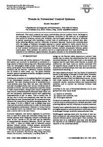
. q(t) where Ri (t) = + Tpi is the round trip time, pi (t) = Kp q(t − Ri (t)) and Cr Tpi is the constant propagation delay. The induced time-delay is τi = 12 Ri (t) and the router output link capacity are supposed to be constant. Example 1. The network consists of one router and two TCP flows (the one used by the system and the controller, and a disturbing one, acting between t = 10s and t = 25s). Its parameters are such that the time-delay is obtained from the following dynamics 1 W1 (t) W1 (t − R1 (t)) dW1 (t) = − p1 (t), dt R1 (t) 2 R1 (t − R1 (t))

E. Witrant, D. Georges, C. Canudas-de-Wit, and M. Alamir

q(t) and W1,2 (t) (packets)

16

Average queue length and windows sizes q(t)

W1 (t)

W2 (t)

time (s) Fig. 1.2. Behavior of the network internal states.

dW2 (t) 1 W2 (t) W2 (t − R2 (t)) = − p2 (t), dt R2 (t) 2 R2 (t − R2 (t))

hal-00196856, version 1 - 13 Dec 2007

2

X Wi (t) dq(t) = −300 + , q(0) = 5, dt Ri (t) i=1 τ (t) = R1 (t)/2,

. q(t) . q(t) + 0.001, R2 (t) = + 0.0015, pi (t) = 0.005 × q(t − Ri (t)), with R1 (t) = 300 300 i = 1, 2, and W1 (0) = W2 (0.25) = 10 packets. The behavior of the network internal states q(t), W1 (t) and W2 (t) is presented on figure 1.2. We now detail how the TCP model is used in the computation of the predictor horizon δ(t) to set the control law established in Theorem 5. From the definition of the Ri (t), we have that   1 q(ζ) + Tpcs . τ (ζ) = (1.18) 2 Cr Deriving the previous equation along with (1.17), it follows that   N (ζ) 1  X Wi (ζ) dτ (ζ) = − Cr  , dζ 2Cr i=1 Ri (ζ)

(1.19)

where Ri (ζ) is obtained from q(ζ), N (ζ) is assumed to be known. Both Wi (ζ) and q(ζ) are obtained from the dynamics (1.16)-(1.17): this is done by continuously computing the solutions of (1.16)-(1.17) up to the time t + τ max . ˙ (1.18)-(1.19) can now be substituted in (1.15) to obtain the dynamics δ(t). Example 2. Considering the delay induced by the network corresponding to the previous example, the predictor’s horizon is computed for two different

Delay and predictor’s horizon (s)

1 On the Use of State Predictors in Networked Control Systems

17

δ(t) (dicho.) τ (t)

δ(t) for λ = 10 δ(t) for λ = 100

hal-00196856, version 1 - 13 Dec 2007

time (s) Fig. 1.3. Computation of the predictor’s horizon.

values of λ and compared with the exact value (computed using dichotomy) in figure 1.3. This simulation shows the effectiveness of the proposed estimation to compute the time-varying horizon. The estimated horizon quickly converges toward its exact value (depending on the choice of λ). Finally, the resulting system response is studied for four different control laws: • • • •

state feedback, state predictor with a variable horizon, state predictor with a fixed horizon equal to the maximum delay, a buffer strategy, where a buffer is added at the system’s input in order to make the delay constant (equal to its maximum value τmax ), combined with the previous predictor.

In order to compare these methods, the system response to a non-zero initial condition and with measurement noises (white vibration of power 0.01 and core [23341]) are illustrated by the figure 1.4. The temporal evolution of the pendulum angle shows that, compared to the use of a predictor with a variable horizon: •

the simple state feedback induces an overshoot and light oscillations when the initial condition is non-zero, and significant oscillations when a measurement noise is added, • the state predictor with a fixed horizon, although more suitable than the previous strategy, induces some oscillations and a longer settling time. It is also more sensitive to measurement noises, • the buffer strategy exhibits a quickly compensated initial divergence (due to the increased delay) and has similar performances as the predictor with a variable horizon (peak slightly weaker). This strategy has the advantage of being simpler from the control point of view but introduces an additional complexity on the system site.

18

E. Witrant, D. Georges, C. Canudas-de-Wit, and M. Alamir 4 3.5

predictor with a variable horizon

θ(t) (rad)

3

state feedback

2.5

predictor with a fixed horizon

2 1.5 1

buffer strategy

0.5 0 −0.5

0

0.2

0.6

0.8

1

predictor with a variable horizon buffer strategy

10

θ(t) (rad)

time (s)

Simulation with measurement noise

15

hal-00196856, version 1 - 13 Dec 2007

0.4

5 0 −5

−10 −15

predictor with a fixed horizon state feedback 0

0.2

0.4

0.6

0.8

time (s) Fig. 1.4. Comparison between different control laws.

1

Note that the previous effects are amplified for delays of more significant amplitude and/or variation. Some experimental results [9] have shown that the state feedback can’t stabilize the system in the real case and a bad transient response, due to some high frequency noise in the control signal, is obtained if the fixed horizon predictor or the buffer strategy is used.

1.6 Conclusion In this chapter, the problem of stabilisation through networks has been formulated as the problem of stabilizing a system with a time-varying delay in the input. The commandability and finite spectrum assignement issues were presented, along with an overview on the use of state predictors in various control scheme. The explicit use of the network dynamics in the design of

1 On the Use of State Predictors in Networked Control Systems

19

the control law was emphasized and illustrated by some simulation examples, where three predictor-based control laws are compared.

1.7 Acknowledgements This study was realized within the NECS-CNRS projet. The authors would like to thank the CNRS for partially funding the project. The authors would also like to thank Jean-Pierre Richard and Rodolphe S´epulchre for their careful reading and constructive remarks on this document.

hal-00196856, version 1 - 13 Dec 2007

References 1. O. Smith, “Closer control of loops with dead time,” Chem. Eng. Prog., vol. 53, pp. 217–219, 1959. 2. S. Niculescu, E. Verriest, L. Dugard, and J.-M. Dion, “Stability and robust stability of time-delay systems: a guide tour,” in Lecture Notes on Control and Information Sciences 228: Stability and Control of Time-delay Systems, L. Dugard and E. Verriest, Eds. New York: Berling Springer, 1998. 3. E. Fridman and U. Shaked, “Delay-dependent stability and H∞ control: constant and time-varying delays,” Int. J. Control, vol. 76, No. 1, pp. 48–60, 2003. 4. R. Yu, “On stability of linear systems with time-varying delay: generalized lyapunov equation,” IEEE AFRICON, vol. 1, pp. 569–574, 1999. 5. E. Verriest, “Stability of systems with state-dependant and random delays,” IMA Journal of Mathematical Control and Information, vol. 19, pp. 103–114, 2002. 6. A. S. Tanenbaum, Computer Networks. Upper Saddle River, New Jersey 07458: Prentice Hall, Inc., 1996. 7. A. Olbrot, “On controllability of linear systems with time delays in the control,” IEEE Trans. Automat. Contr., vol. ac-16, pp. 664–666, 1972. 8. S. Mondi´e and W. Michiels, “A safe implementation for finite spectrum assignment: robustness analysis,” in Proceedings of the 42nd IEEE Conference on Decision and Control (CDC2003), Hawaii, USA, Dec. 2003. 9. E. Witrant, “Stabilisation des syst`emes command´es par r´eseaux.” Ph.D. dissertation, INPG/Laboratoire d’Automatique de Grenoble, Grenoble, France, Sept. 2005. 10. A. Manitius and A. Olbrot, “Finite spectrum assignment problem for systems with delays,” IEEE Trans. Automat. Contr., vol. 24, pp. 541–552, Aug. 1979. 11. W. Kwon and A. Pearson, “Feedback stabilization of linear systems with delayed control,” IEEE Trans. Automat. Contr., vol. ac-25, no.2, pp. 266–269, Apr. 1980. 12. Z. Artstein, “Linear systems with delayed control: a reduction,” IEEE Trans. Automat. Contr., vol. ac-27, no.4, pp. 869–879, Aug. 1982. 13. M. Nihtil¨ a, “Adaptive control of a continuous-time system with time-varying input delay,” Systems and Control Letters, no. 12, pp. 357–364, 1989. 14. ——, “Finite pole assignment for systems with time-varying input delays,” in Proc. of the 30rd IEEE Int. Conf. on Decision and Control, Brighton, England, Dec. 1991.

hal-00196856, version 1 - 13 Dec 2007

20

E. Witrant, D. Georges, C. Canudas-de-Wit, and M. Alamir

15. ——, “Pole placement design methodology for input delay systems,” in European Control Conference, Grenoble, France, July 1991. 16. S. Mondi´e, S. Niculescu, and J.-J. Loiseau, “Delay robustness of closed loop finite assignment for input delay systems,” in Proc. of the 3rd IFAC Conference on Time Delay Systems, Santa Fe, New Mexico, USA, Dec. 2001. 17. K. Uchida, Y. Misaki, T. Azuma, and M. Fujita, “Predictive H ∞ control for linear systems over communication channels with time-varying delays,” in Proc. of the 4th IFAC Workshop on Time Delay Systems, Rocquencourt, France, Sept. 2003. 18. T. A. K. Uchida, K. Ikeda and A. Kojima, “Finite-dimensional characterizations of H ∞ control for linear systems with delays in control input and controlled output,” in Proc. of the 2nd IFAC Workshop on Time Delay Systems, Ancona, USA, 2000, pp. 219–224. 19. E. Witrant, D. Georges, C. Canudas-de-Wit, and O. Sename, “Stabilisation of network controlled systems with a predictive approach,” in Proc. of the 1 st Workshop on Networked Control System and Fault Tolerant Control, Ajaccio, France, Oct. 2005. 20. E. Witrant, C. Canudas-de-Wit, and D. Georges, “Remote output stabilization under two channels time-varying delays,” in Proc. of the 4th IFAC Workshop on Time Delay Systems, Rocquencourt, France, Sept. 2003. 21. S. Hirche and M. Buss, “Telepresence control in packet switched communication networks,” in Proc. of the IEEE Conference on Control Applications, Taipei, Taiwan, Sept. 2004. 22. V. V. Assche, M.Dambrine, J.-F. Lafay, and J.-P. Richard, “Some problems arising in the implementation of distributed-delay control laws,” in Proc. of the 38th Conference on Decision and Control, Phoenix, Arizona (USA), Dec. 1999. 23. A. Fattouh, O. Sename, and J.-M. Dion, “Pulse controller design for linear systems with delayed state and control,” in Proc. of the 1st IFAC Symposium on System Structure and Control, Prague, Czeck Republic, 2001. 24. R. B. Sidje, “Expokit: a software package for computing matrix exponentials,” ACM Transactions on Mathematical Software (TOMS), vol. 24, no. 1, pp. 130– 156, March 1998. 25. P. Borne, G. Dauphin-Tanguy, J.-P. Richard, F. Rotella, and I. Zambettakis, Modlisation et identification des processus. Tome 1, ser. Mthodes et Pratiques de l’Ingnieur. Paris (France): Technip, 1992. 26. E. Witrant, C. Canudas-de-Wit, D. Georges, and M. Alamir, “Remote stabilization via time-varying communication network delays: Application to TCP networks,” in Proc. of the IEEE Conference on Control Applications, Taipei, Taiwan, Sept. 2004. 27. V. Misra, W.-B. Gong, and D. Towsley, “Fluid-based analysis of a network of AQM routers supporting TCP flows with an application to RED,” in Proc. of ACM SIGCOMM’00, Stockholm, Sweden, Sept. 2000. 28. C. Hollot and Y. Chait, “Nonlinear stability analysis for a class of TCP/AQM networks,” in Proc. of the 40th IEEE Int. Conf. on Decision and Control, Orlando, Florida, USA, Dec. 2001.

Index

finite spectrum assignment, 8

hal-00196856, version 1 - 13 Dec 2007

network, 1–4, 12, 15 networked control systems, 1 observer-based control, 12

predictive control, 1, 11 Smith predictor, 1 state predictor, 2, 6, 8, 10 TCP, 15, 16 time-varying delay, 1, 8, 11