Unsupervised Traffic Flow Classification Using a Neural Autoencoder Jonas H¨ochst∗† , Lars Baumg¨artner∗ , Matthias Hollick† , Bernd Freisleben∗† ∗ Department
of Mathematics & Computer Science, Philipps-Universit¨at Marburg, Germany E-mail: {hoechst, lbaumgaertner, freisleb}@informatik.uni-marburg.de † Department of Computer Science / Electrical Engineering & Information Technology, TU Darmstadt, Germany E-mail:
[email protected], {jonas.hoechst, bernd.freisleben}@maki.tu-darmstadt.de
Abstract—To cope with the varying delay and bandwidth requirements of today’s mobile applications, mobile wireless networks can profit from classifying and predicting mobile application traffic. State-of-the-art traffic classification approaches have various disadvantages: port-based classification methods can be circumvented by choosing non-standard ports, protocol fingerprinting can be confused by the use of encryption, and current supervised learning methods for analyzing the statistical properties of network flows try to detect predefined classes, such as e-mail or FTP traffic, learned during training. In this paper, we present a novel approach to unsupervised traffic flow classification using statistical properties of flows and clustering based on a neural autoencoder. A novel time interval based feature vector construction and a semi-automatic cluster labeling method facilitate traffic flow classification independent of known traffic classes. An experimental evaluation on real data captured over a period of four months is presented. The obtained results show that 7 different classes of mobile traffic flows are detected with an average precision of 80% and an average recall of 75%. Index Terms—Autoencoder, Traffic flow classification, Unsupervised learning
I. I NTRODUCTION The growing popularity of smartphone and tablet usage poses challenging demands on mobile communication. Apart from browsing the web, real-time and high-bandwidth services, such as Voice-over-IP (VoIP) or video live streaming, are increasingly used in today’s mobile applications. With the paradigm shift towards Software-Defined Networking (SDN) in the network core and Software-Defined Wireless Networking (SDWN) in the network edge [1], dynamic flow configurations can heavily profit from network traffic classification for priorization and resource management. Currently, Internet traffic classification is used to improve Quality-of-Service (QoS) or Quality-of-Experience (QoE) [2], [3]. Traffic classification methods can be grouped into portbased, payload-based and statistical methods [4]. Since many applications do not rely on fixed port numbers and ports can be easily redirected or obfuscated, port-based methods are inadequate for characterizing the properties of network traffic. Payload-based methods use certain fields of application layer protocols to classify traffic. In particular, Deep Packet Inspection (DPI) uses fixed protocol signatures of the packet payload [3], [5]. However, payload-based methods fail whenever connections are encrypted. Furthermore, they can be
easily circumvented, and changes of the application protocols may also lead to false classifications. Statistical approaches [6], [7], [8], [9] typically use packet inter-arrival times, packet sizes and their statistical properties (e.g., average, maximum, minimum). They often rely on machine learning algorithms for performing traffic classification, in particular supervised learning algorithms that require labeled data for training to build a suitable classification model. The labels are often obtained from validated application ports or other labeling mechanisms (such as DPI), resulting in classification mechanisms that replicate the labeling methods, rather than revealing new structures independent of prior knowledge. In many cases, web browsing is equated with HTTP(S) traffic, while Skype traffic is assigned to video conferences. This is misleading in various ways, since nowadays HTTP(S) is the basis for many applications other than browsing the web. In this paper, we present a novel approach to unsupervised traffic flow classification using statistical properties of flows and clustering based on a neural autoencoder. In contrast to previous work, the neural autoencoder is used to automatically cluster traffic flows, e.g., into downloads, uploads, or voice calls, independent of the particular network protocols, such as FTP or HTTP(S), used for performing these tasks. A novel time interval based feature vector construction is proposed. By separating flows into exponentially growing time periods and computing their statistical properties individually, a weighted bandwidth graph is fed into the neural autoencoder. A semiautomatic cluster labeling method facilitates traffic flow classification independent of known traffic classes. An experimental evaluation on real data captured from about 25 mobile devices performing daily work over a period of 4 months is presented. The obtained results show that 7 different classes of mobile traffic flows are detected sufficiently fast with an average precision of 80% and an average recall of 75%. II. R ELATED W ORK The survey of Nguyen and Armitage [2] compares the results of various machine learning approaches applied to network traffic classification. Traffic classification based on machine learning is still an open field [10]. Classification approaches based on multiple identification methods reaching from packet headers to full flow examination
traffic (bytes/s)
6000
800
5000
600
4000 3000
400
2000
200
1000 0
1000
0
20
40
60 time (s)
80
(a) Audio call
100
0 120
250000
1600
forward backward 1400
200000
1600
forward backward 1400
100000
1200 1000
150000
800 100000
600
1200 80000
1000
60000
800 600
40000
400
50000
200 0
120000
0
10
20
30 time (s)
40
50
(b) Website interaction
60
0
packet size (byte)
7000
1200
packet size (byte) traffic (bytes/s)
forward backward
8000
packet size (byte) traffic (bytes/s)
9000
400 20000 0
200 0
20
40
time (s)
60
80
0
(c) Buffered videostream
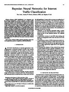
Fig. 1: Traffic utilization and packet sizes of example flows.
and even host history inclusion have been presented [11], [7] to classify traffic into 10 classes, such as INTERACTIVE, MAIL, WWW or MULTIMEDIA. Moore et al. [6] use Bayesian analysis techniques with 248 per-flow features to reach a basic classification accuracy of 65%. By improving the basic methods, 95% classification accuracy is reached. Kim et al. [12] criticize the high variability in data sources and classification targets. The authors propose to use overall accuracy, precision, recall and F-Measure as performance metrics, as well as 4 different publicly available datasets created between 2004 and 2006. They also compare different machine learning approaches and reach 94.2%-97.8% accuracy using a Support Vector Machine (SVM) [13]. Semi-supervised methods have been proposed [7] to find clusters of traffic flows using the K-means algorithm [14]. The clusters are labeled afterwards using a small set of labeled flows. The authors also propose a real-time classification method where multiple layers offer classifications based on packet milestones. Vladutu et al. [15] present a semisupervised framework for flow classification using generated traffic and thus the resulting semantic categories. Zhang et al. [9] present an unsupervised clustering algorithm based on statistical properties of flows as well as payloadbased clustering. The authors use 13 different classes as their ground truth, made up of different protocols, such as HTTP and SSH. The flows are clustered using several configurations of the K-means algorithm. The majority of methods proposed in the literature are based on supervised learning methods. Using unsupervised clustering instead, the methods do not rely on the ground truth of the labeling mechanisms. Clearly, at some point labels have to be attached to be able to compare the mechanisms, but the actual learning is independent of pre-labeled flows that are hard to obtain in good quality and/or high numbers [2], [9]. III. A N EURAL AUTOENCODER FOR T RAFFIC F LOW C LASSIFICATION This section presents the design of the proposed neural autoencoder for traffic flow classification. A. Feature Vector Construction We try to keep the number of statistical features low to reduce computational demands and memory usage. In addi-
tion to statistical features, such as number of packets/bytes, avg./stdev. packet size and inter-arrival time etc., the median of the Differentiated Services Codepoint (DSCP) field is used. This IP header field is a successor of the Type-of-Service (ToS) field and is used to indicate network demands of packets. All features are computed in each flow direction, namely forward (client to server) and backward (server to client). For TCP flows, clients and servers are defined by the connection handshake. Since UDP is a connection-less protocol, a UDP flow is defined as a repeated exchange of packets between the same sender IP/port and recipient IP/port combination. In Figure 1, three examples of network flows are presented. The red and blue lines show the forward and backward traffic. Each red and blue dot stands for a single TCP forward or backward packet, respectively. Comparing the presented examples, great differences in bandwidth consumption, interarrival times and packet sizes can be observed. For Figure 1a and Figure 1c, the most important criteria for clustering are available after a short period of time. This perception can be used to improve flow clustering, in particular with respect to future online classification. To use this knowledge, the feature vector is constructed using exponentially growing time periods for statistical flow property computation. In this way, information from the beginning of flows is less reduced compared to information from the later parts. Using this method, it is also possible to constitute the duration information of flows while using a fixed length feature vector, as required by most machine learning algorithms. The feature vector used in this paper is constructed using exponentially growing intervals of up to 2048 seconds. There are two possible computation methods. In the cumulative method, the interval boundaries range from the beginning of the flow until the end boundary. The used values are statistical properties up to the current time. The second method is non-cumulative and therefore each interval only contains the statistical information of packets handled in the interval itself. In total, each feature vector has 216 features: 2 half flows * 12 intervals * 9 statistical features. B. Clustering via a Neural Autoencoder Neural autoencoders [16], [17] are useful for dimension reduction and classification. The general approach of neural
TABLE I: Manually extracted classes Class Browsing Interactive Download Livestream Videostream Call
Principal feature ephemeral long lasting large downstream constant bitrate periodic buffering low iat, symmetric
Upload
large upstream
Example mobile application Wikipedia, Spiegel, Heise Online Games, Facebook, Twitter Updates, Dropbox Streaming, iTunes Webradio Youtube, Vimeo, Facebook, Twitch Skype, Apple FaceTime, Google Hangouts, WhatsApp YouTube, Facebook, WhatsApp
entering a command, leads to a back flow of data. The last example is presented in Figure 1c. It shows the flow properties of a buffered video stream. In modern audio/video streaming protocols (e.g., Apple HLS, MPEG DASH), segments of the stream are delivered as individual files. If the local buffer runs low, another segment is downloaded. IV. I MPLEMENTATION In this section, the implementation of our network traffic classification approach is presented.
autoencoders is a model that is trained to reconstruct an original input vector from a smaller representation. It is trained using the squared reconstruction error as its cost function. The classification approach consists of multiple steps. First, the feature vector is normalized using the standard score. While this seems to be the preferred mode, mean-only, standard deviation-only and no standardization are also evaluated in our approach, to potentially save computational overhead. The resulting vector is mainly used to train the autoencoder and afterwards only for feature encoding. Then, the Softmax (normalized exponential) function is applied to the encoded values. The actual class is then determined by selecting the index of the greatest element in the Softmax vector. This method is a rather modest classification method with the advantage of producing highly differing cluster sizes. Our autoencoder is trained using the summed squared error in combination with the Adaptive Moment Estimator (Adam)[18].
A. Data Capture
C. Cluster Labeling
C. Neural Autoencoder and Classification
The obtained clusters from the previous step need to get a semantic label. Therefore, we use a semi-automatic method comparable to Zhang et al. [9] and Vladutu et al. [15]. Both labeling methods obtain a ground truth set of labeled flows. Zhang et al.[9] use application layer protocols, while Vladutu et al. [15] use generated traffic and thus the applications’ names as the ground truth. Both methods have disadvantages in generalizing their classification approach, since only cherrypicked protocols are investigated. To overcome these disadvantages, we have defined our own set of classes, based on the clusters extracted by the neural autoencoder and popular application categories. These 7 classes, their main features and examples of mobile applications, namely Browsing, Interactive, Download, Livestream, Videostream, Call and Upload, are presented in Table I. Figure 1a shows an example of a flow from the Call class. The primary features of a low inter arrival time and relatively low but varying packet sizes are visible in the figure. While the backward bandwidth is continuously above 5 kB/s, the forward bandwidth keeps dropping to very low values. In Figure 1b, an example flow of browsing Twitter is presented. Peaks in backward bandwidth of up to 200 kB/s are visible, while the forward bandwidth stays pretty low. This graph is typical for user interactions with either social networks or even remote server management, e.g., via SSH. A relatively small amount of input data, e.g., scrolling, clicking,
To implement the presented neural autoencoder, the open source library TensorFlow2 is used. The labeled data is clustered using the already trained network. The cluster then gets assigned the most frequent label from the previously labeled data. If there are clusters that contain no labels, no cluster label is assigned and the cluster may need further manual inspection.
The data used in our work was captured in an office network used by roughly 10 users including 5 frequent users with an overall count of roughly 25 devices. The data was captured in two phases. In the first phase, traffic was captured on both wireless interfaces with 12.7 GB used over the 2.4 GHz network and 36.8 GB transferred via the 5 GHz network over a three months period. In the second phase, all traffic was captured, explicitly including wired machines. Local traffic was excluded from all sets, resulting in 30 GB over a one month period. B. Data Processing In the first step, the tool pkt2flow1 splits up the input file to one pcap per flow before the statistical values of flows are computed. The cluster labeling is implemented in the same way as proposed by Zhang et al. [9] and Vladutu et al. [15].
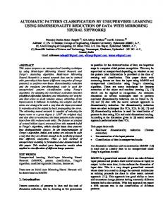
V. E XPERIMENTAL E VALUATION In this section, the proposed method is evaluated. a) Aggregation Method: Two aggregation methods were examined. The cumulative method (cum) is around 15% worse than using the non-cumulative version (noncum), where the flow is separated into multiple segments and the statistical values are computed individually. b) Number of Clusters: The number of clusters is defined by the number of hidden nodes of our neural autoencoder. In our parameter scan, we evaluated 10, 15, 20, 30, 40, 60, 80 and 100 clusters. The experiment shows (Fig. 2) that a sweet spot can be identified when 60 clusters are used, since the averaged results are not significantly better when more clusters are used. c) Scaler: The scaler has a major impact on the classification results. While average precision and recall are only at roughly 50% when no scaler is used, the standard scaler improves average precision and recall up to around 60%. 1 https://github.com/jonashoechst/pkt2flow 2 https://www.tensorflow.org
TABLE II: Classification quality
60% 55% 50% 45% 40%
10 15 20
30
40
60 number of clusters
avg precision avg recall avg f1-score 80 100
Fig. 2: Classification quality vs. number of clusters
d) Classification Quality: Table II shows the obtained classification quality. The neural autoencoder in the configuration with 100 clusters, learning in 30 epochs with a standard scaler based on the full dataset produced the best result. These 100 clusters are mapped by our classifier to our 7 chosen classes. An average precision of 80% and an average recall of 75% are achieved, which results in an F1 score of 76%. e) Execution Time: Our runtime experiments were performed on a 2 x 2.26 GHz Intel Xeon quad-core machine. While the generation of flow objects from the pcap file took around 2.20 ms per flow and the computation of the feature vectors took about 1.67 ms per flow, the actual classification only took 0.006 ms per flow. With a rate of over 200,000 flows per second, our method can be used at the network edges, where access points or mobile devices themselves can classify the traffic and dynamically change connection properties using SDN and SDWN technology to ensure optimal resource usage. VI. C ONCLUSION In this paper, we have presented a novel approach to unsupervised traffic flow classification using statistical properties of flows and clustering based on a neural autoencoder that has been used to cluster traffic flows into downloads, uploads, calls, browsing, videostream, live stream or interactive communication, independent of the particular network protocols used for performing these tasks. A novel time interval based feature vector construction and a semi-automatic cluster labeling method have facilitated traffic flow classification independent of known traffic classes. Our evaluation using four months of captured traffic has shown that our 7 classes of traffic flows are detected sufficiently fast with an average precision of 80% and an average recall of 75%. There are several areas for future work, such as (a) using deep and especially stacked autoencoders [19] to improve the mapping of classes to clusters, (b) replacing the SoftMax classification method by other methods to improve the classification, and (c) training the network with subflows of varying lengths to use our approach for nearly real-time classification after observing only a few seconds of the packet stream. ACKNOWLEDGMENT This work is funded by the LOEWE initiative (Hessen, Germany) within the NICER project and the Deutsche Forschungsgemeinschaft (DFG, SFB 1053 - MAKI).
videostream upload livestream browsing download call interactive avg/total
precision 0.47 1.00 0.86 0.91 0.80 0.87 0.71 0.80
recall 0.80 0.85 0.67 0.50 0.80 1.00 0.60 0.75
F1 score 0.59 0.92 0.75 0.65 0.80 0.93 0.65 0.76
R EFERENCES [1] C. J. Bernardos, A. De La Oliva, P. Serrano, A. Banchs, L. M. Contreras, H. Jin, and J. C. Z´un˜ iga, “An architecture for software defined wireless networking,” IEEE Wireless Communications, vol. 21, no. 3, pp. 52–61, 2014. [2] T. T. Nguyen and G. Armitage, “A survey of techniques for internet traffic classification using machine learning,” IEEE Communications Surveys & Tutorials, vol. 10, no. 4, pp. 56–76, 2008. [3] B. Li, J. Springer, G. Bebis, and M. H. Gunes, “A survey of network flow applications,” Journal of Network and Computer Applications, vol. 36, no. 2, pp. 567–581, 2013. [4] A. Dainotti, A. Pescape, and K. C. Claffy, “Issues and future directions in traffic classification,” IEEE Network, vol. 26, no. 1, 2012. [5] T. Qin, L. Wang, Z. Liu, and X. Guan, “Robust application identification methods for p2p and voip traffic classification in backbone networks,” Knowledge-Based Systems, vol. 82, pp. 152–162, 2015. [6] A. W. Moore and D. Zuev, “Internet traffic classification using Bayesian analysis techniques,” in ACM SIGMETRICS Performance Evaluation Review, vol. 33, no. 1. ACM, 2005, pp. 50–60. [7] J. Erman, A. Mahanti, M. Arlitt, I. Cohen, and C. Williamson, “Semisupervised network traffic classification,” in ACM SIGMETRICS Performance Evaluation Review, vol. 35, no. 1. ACM, 2007, pp. 369–370. [8] J. Zhang, X. Chen, Y. Xiang, W. Zhou, and J. Wu, “Robust network traffic classification,” IEEE/ACM Transactions on Networking (TON), vol. 23, no. 4, pp. 1257–1270, 2015. [9] J. Zhang, Y. Xiang, W. Zhou, and Y. Wang, “Unsupervised traffic classification using flow statistical properties and IP packet payload,” Journal of Comp. and Syst. Sciences, vol. 79, no. 5, pp. 573–585, 2013. [10] N. Namdev, S. Agrawal, and S. Silkari, “Recent advancement in machine learning based internet traffic classification,” Procedia Computer Science, vol. 60, pp. 784–791, 2015. [11] A. W. Moore and K. Papagiannaki, “Toward the accurate identification of network applications,” in International Workshop on Passive and Active Network Measurement. Springer, 2005, pp. 41–54. [12] H. Kim, K. C. Claffy, M. Fomenkov, D. Barman, M. Faloutsos, and K. Lee, “Internet traffic classification demystified: myths, caveats, and best practices,” in Proceedings of the 2008 ACM CoNEXT Conference. ACM, 2008, pp. 11:1–11:12. [13] V. N. Vapnik and A. J. Chervonenkis, Theory of pattern recognition. Nauka, 1974. [14] S. Lloyd, “Least squares quantization in PCM,” IEEE Transactions on Information Theory, vol. 28, no. 2, pp. 129–137, 1982. [15] A. Vl˘adut¸u, D. Com˘aneci, and C. Dobre, “Internet traffic classification based on flows’ statistical properties with machine learning,” International Journal of Network Management, 2016. [16] C. Song, F. Liu, Y. Huang, L. Wang, and T. Tan, “Auto-encoder based data clustering,” in Iberoamerican Congress on Pattern Recognition. Springer, 2013, pp. 117–124. [17] P. Huang, Y. Huang, W. Wang, and L. Wang, “Deep embedding network for clustering,” in 22nd International Conference on Pattern Recognition (ICPR). IEEE, 2014, pp. 1532–1537. [18] D. Kingma and J. Ba, “Adam: A method for stochastic optimization,” arXiv preprint arXiv:1412.6980, 2014. [19] P. Vincent, H. Larochelle, I. Lajoie, Y. Bengio, and P.-A. Manzagol, “Stacked denoising autoencoders: Learning useful representations in a deep network with a local denoising criterion,” Journal of Machine Learning Research, vol. 11, no. Dec, pp. 3371–3408, 2010.