Using ASME format - Microelectronics Heat Transfer Laboratory

J. R. Culham Associate Professor and Director, Mem. ASME,

M. M. Yovanovich Professor Emeritus and Principal Scientific Advisor, Fellow ASME, Microelectronics Heat Transfer Laboratory, Department of Mechanical Engineering, University of Waterloo, Waterloo, Canada

T. F. Lemczyk Project Engineer, Louisiana State University, Baton Rouge, LA 70821

Thermal Characterization of Electronic Packages Using a Three-Dimensional Fourier Series Solution The need to accurately predict component junction temperatures on fully operational printed circuit boards can lead to complex and time consuming simulations if component details are to be adequately resolved. An analytical approach for characterizing electronic packages is presented, based on the steady-state solution of the Laplace equation for general rectangular geometries, where boundary conditions are uniformly specified over specific regions of the package. The basis of the solution is a general threedimensional Fourier series solution which satisfies the conduction equation within each layer of the package. The application of boundary conditions at the fluid-solid, packageboard and layer-layer interfaces provides a means for obtaining a unique analytical solution for complex IC packages. Comparisons are made with published experimental data for both a plastic quad flat package and a multichip module to demonstrate that an analytical approach can offer an accurate and efficient solution procedure for the thermal characterization of electronic packages. 关S1043-7398共00兲01403-1兴

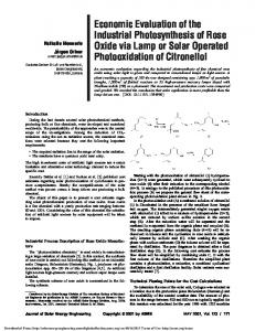
Introduction The accurate prediction of component junction temperatures in electronic packages can lead to complex and time consuming simulations. Although analytical techniques can provide accurate and expedient solution methods, it is generally perceived that the complex geometries associated with microelectronic packaging do not lend themselves to analytical procedures. Many researchers have used finite Fourier transform techniques to solve the heat conduction problem in multilayer structures found in integrated circuits. The solution procedures are generally limited to two- and three-dimensional analyses in geometrically conforming laminates as shown in Fig. 1. Through the selective application of appropriate boundary conditions, the solution procedures for conforming laminated structures can be easily modified to include the nonconforming structures found in many electronic packages. Gray 关1兴 and Kokkas 关2兴 present steady-state and transient solutions, based on Fourier and Laplace transform techniques, for determining temperatures in a three-dimensional multilayer substrate. Lemczyk et al. 关3兴 use a Fourier series solution to solve the three-dimensional heat conduction problem in a multilayer printed circuit board. The analytical approach used in all of these procedures is discussed in Carslaw and Jaeger 关4兴. Albers 关5兴 introduces a recursion technique for improving the solution efficiency of Fourier transform methods in both rectangular and cylindrical multilayered structures. While all of these solutions can predict temperature or heat flux for any point in a three-dimensional field they are restricted to simple, rectangular laminates which do not resemble the more complex geometries found in any of the package geometries shown in Fig. 2. Since the primary role of an electronic package is to provide protection to the sensitive components on the surface of the integrated circuit, the IC is generally fully encapsulated within a plastic or ceramic structure. The IC or die is bonded to a leadframe, which provides electrical pinout connections and an excellent path for dissipating excess heat. While some packages, such as plastic,

dual inline packages, fully encase the IC in a plastic mold, others such as ceramic quad flat packs, have an internal cavity where the IC can be attached to either the lower or upper surface surrounding the cavity. Conventional analytical models based on Fourier transform methods do not conform well to these complex geometries, found in most electronic packages. The purpose of this paper is to present a modeling procedure that uses finite Fourier transform methods to simulate heat transfer in many of the package geometries used in present day microelectronic applications. While the analyses can be detailed, a general overview of the governing equations, boundary conditions, and solution procedures will be presented. A full solution, including the equation development and the approach used to code the solution, is presented by Lemczyk et al. 关6兴. The basis of the solution is a general three-dimensional Fourier series solution which precisely satisfies the conduction equation within each layer of the package. The application of boundary conditions at fluid-solid, package-board and layer-layer interfaces provides a means for obtaining a unique analytical solution for complex IC packages. It will be demonstrated by comparison to published experimental data that an analytical approach can offer an accurate and time efficient solution procedure for the thermal characterization of electronic packages.

Contributed by the Electrical and Electronic Packaging Division for publication in the JOURNAL OF ELECTRONIC PACKAGING. Associate Technical Editor: R. Wirtz.

Journal of Electronic Packaging

Copyright © 2000 by ASME

Fig. 1 Multiple layer substrate

SEPTEMBER 2000, Vol. 122 Õ 233

Fig. 2 Various package geometries reproduced from sketches in Bar-Cohen †11‡

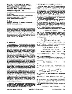
Modeling Procedure Assumptions. Several assumptions have been used in the development of a thermal model for simulating microelectronic packages. Each of the assumptions is selected to simplify the mathematical calculations while preserving the physical integrity of the problem as much as possible. The analysis is based on the solution to Laplace’s equation, where heat is produced at the top surface of the die plane layer and there are no other sources of internal heat generation. The source of heat, typically a silicon wafer, is assumed to be infinitely thin with uniform heat generation. The layers within the various sections of the package structure are assumed to be composed of homogeneous, isotropic materials of known thickness and thermal conductivity. This implies that layers, such as the lead frame, where the layer may consist of both a metallic frame and a plastic or ceramic binder, are considered to have a single value of thermal conductivity over the full extent of the layer. Adjacent layers are assumed to be in perfect contact, where the contact resistance between layers is considered negligible and the temperature and the heat flux are equated across the interface. The convective boundary conditions over the upper and lower surfaces of the package are assumed to be uniform. Each layer exposed along the sidewalls of the package can have a unique, uniformly specified convective boundary condition. Single Layer Model. A basic three-dimensional rectangular, planar layer with a local coordinate reference is used to represent each layer. The overall length of the layer is L 1 and the overall width, L 2 as shown in the multilayer package in Fig. 3. The layer is assumed to have a homogeneous thermal conductivity k i , and each exposed side face of the layer, numbered 1–4, has a uniquely specified boundary condition, denoted as h j,i and T i where j refers to the particular side 共1–4兲 and i refers to the layer number. The controlling governing partial differential equation for three-dimensional steady state heat transfer in a rectangular, homogeneous body with no internal heat sources is Laplace’s equation, given as

⳵ 2␪ ⳵ 2␪ ⳵ 2␪ ⫹ ⫹ ⫽0 ⳵x2 ⳵y2 ⳵z2

(1)

␪ ⫽T⫺T a

(2)

Fig. 3 Coordinate system for package model

For practical engineering purposes, the infinite series specified in terms of m and n in Eq. 共3兲 are truncated to an upper limit N which can be arbitrarily specified subject to accuracy requirements and problem specific conditions. Typical values of m and n are in the range of 10–30, with an accuracy advantage obtained for higher values of the truncation limit along with a corresponding penalty in calculation time N

␪ i 共 x,y,z 兲 ⫽

N

兺 兺 X 共 x 兲Y 共 y 兲Z 共 z 兲 i

m⫽1 n⫽1

L1 L1

␪ i 共 x,y,z 兲 ⫽

兺 兺 X 共 x 兲Y 共 y 兲Z 共 z 兲

m⫽1 n⫽1

i

234 Õ Vol. 122, SEPTEMBER 2000

i

i

(3)

(4)

L2

⳵␪i ⫺Bi1,i ␪ i ⫽0; x⫽0 ⳵x

(5)

⳵␪i ⫹Bi2,i ␪ i ⫽0; ⳵x

x⫽L 1

(6)

⳵␪i ⫺Bi3,i ␪ i ⫽0; ⳵y

y⫽0

(7)

⳵␪i ⫹Bi4,i ␪ i ⫽0; ⳵y

y⫽L 2

(8)

L2

where Bi1,i ⫽

h 1,i L 1 ; ki

h 3,i L 2 ; Bi3,i ⫽ ki

Bi2,i ⫽

h 2,i L 1 ki

(9)

h 4,i L 2 Bi4,i ⫽ ki

The separation functions in Eq. 共4兲, and the characteristic roots which automatically satisfy the boundary conditions in Eqs. 共5兲– 共8兲 are defined as

and T a is assumed to be a uniform ambient temperature which is specified for the four sides of each layer. An exact, separable series solution for Eq. 共1兲 can be written for the temperature rise within each layer as ⬁

i

The four sides of each layer are subject to a uniform, convective boundary condition, such that

where

⬁

i

X i 共 x 兲 ⫽cos共 ⑀ m,i x/L 1 兲 ⫹

Bi1,i sin共 ⑀ m,i x/L 1 兲 ⑀ m,i

(10)

Y i 共 y 兲 ⫽cos共 ␭ n,i y/L 2 兲 ⫹

Bi3,i sin共 ␭ n,i y/L 2 兲 ␭ n,i

(11)

i兲 i兲 Z i 共 z 兲 ⫽a 共m,n cosh共 ␥ m,n z/L 1 兲 ⫹b 共m,n sinh共 ␥ m,n z/L 1 兲

⑀ m,i :

(12)

2 ⫺Bi1,i Bi2,i 兲 sin共 ⑀ m,i 兲 ⫺ ⑀ m,i 共 Bi1,i ⫹Bi2,i 兲 cos共 ⑀ m,i 兲 ⫽0 共 ⑀ m,i

(13) Transactions of the ASME

␭ n,i :

2 ⫺Bi3,i Bi4,i 兲 sin共 ␭ n,i 兲 ⫺␭ n,i 共 Bi3,i ⫹Bi4,i 兲 cos共 ␭ n,i 兲 ⫽0 共 ␭ n,i (14) i兲 ␥ 共m,n ⫽

冑 冉 2 ⑀ m,i ⫹

L1 ␭ L 2 n,i

冊

(15)

(16)

where h botL 1 Bibot⫽ k1

(17)

⌰ bot⫽T bot⫺T s,1

(18)

The boundary condition is applied over the full planar surface 0⭐x⭐L 1 , 0⭐y⭐L 2 . Since the boundary condition in Eq. 共16兲 is uniform, the principle of orthogonality for the chosen Fourier series functions 共which are themselves orthogonal functions兲 will directly result in a relationship between the Fourier coefficients in the layer. 1兲 1兲 1兲 共1兲 b 共m,n ⫽ f 共m,n ⫹g 共m,n a m,n

This directly relates (1) (1) f m,n , g m,n , where 1兲 ⫽ f 共m,n

to

(1) b m,n

(19)

through the explicit constants

⫺2 共 Bibot⌰ bot兲 sin共 ⑀ m,1兲 sin共 ␭ n,1兲 1兲 ␥ 共m,n 共 ␭ n,1⫹sin共 2␭ n,1兲 /2兲共 ⑀ m,1⫹sin共 2 ⑀ m,1兲 /2兲 1兲 g 共m,n ⫽

Bibot

(20)

冏

⳵ ␪ i⫹1 ⳵z

⫽␬i z⫽0

冏

⳵␪i ⳵z

m⫽1 n⫽1

共i兲 m,n

冉

N

N

兺兺

m⫽1 n⫽1

ti L1

兺 兺 冉a N

i⫹1 兲 共 i⫹1 兲 b 共m,n ␥ m,n X i⫹1 Y i⫹1 ⫽ ␬ i

冉

i兲 cosh ␥ 共m,n

冊冊

X iY i

N

m⫽1 n⫽1

冉

共i兲 m,n

i兲 i兲 ⫹b 共m,n cosh ␥ 共m,n

ti L1

冉 冊冊

i兲 sinh ␥ 共m,n

ti L1

冊 (26)

ti L1

冊

i兲 X i Y i ␥ 共m,n

(27) Equations 共26兲, 共27兲, and 共19兲 provide the inter-layer relationships needed to determine the Fourier coefficients in each layer in (1) terms of a single, unresolved Fourier coefficient, a m,n . Solution Procedure. For modeling purposes the electronic package, as shown in Fig. 3, has been divided into three distinct zones: 共a兲 Basecell 共b兲 Sidewalls 共c兲 Cap Each of these zones consists of one or more layers with the layer numbering scheme as indicated in Fig. 3. For the case of a fully encased package, the sidewall sections can be omitted, leaving a basecell and a package cap which sits directly on top of the die. The temperature or heat flux solution for a multilayered substrate with either a single heat source, as shown in Fig. 4共a兲 or a multiple heat source configuration, as shown in Fig. 4共b兲, involves the solution of a mixed boundary value problem. The boundary conditions for each discrete section on the planar surface with the sources, referred to as the die plane layer, can be written as

⳵␪M1 ⳵z

⫹Bi j 共 ␪ M 1 ⫺⌰ j 兲 ⫽

q jL1 ; kM1

z⫽t M 1

(28)

where j denotes the section number and

Multilayer Model. Each layer in a multilayered cell has a local coordinate system with a unique origin, which in turn conforms to the above specified equations. The numerical coupling of the governing equations within each layer is attained through the application of two boundary conditions along the common interface, based on the assumption of perfect contact between all adjacent layers. The two boundary conditions are specified such that temperature and heat flux are preserved across the interface at every point in the planar domain.

␪ i⫹1 ⫽ ␪ i ⫹⌰ i

兺 兺 冉a N

i兲 i兲 ⫹b 共m,n sinh ␥ 共m,n

L1

(21)

1兲 ␥ 共m,n

兺兺

N

i⫹1 兲 a 共m,n X i⫹1 Y i⫹1 ⫽⌰ i

2

⳵␪1 ⫺Bibot共 ␪ 1 ⫺⌰ bot兲 ⫽0; z⫽0 ⳵z

(1) a m,n

N

m⫽1 n⫽1

The separation functions X i (x) and Y i (y) are determined based on layer geometry, properties and surface boundary conditions. The only remaining unknowns in the solution are the Fourier co(i) (i) efficients, a m,n and b m,n , which can be determined based on the boundary conditions specified over the upper and lower planar surfaces. In the case of a multilayered structure, the Fourier coefficients in adjacent layers must be coupled in order to impress the influence of the boundary conditions at the upper and lower exposed surfaces throughout the multilayered structure. A relationship between the two Fourier coefficients in a layer can be determined by using the uniformly specified boundary condition over the lower planar surface of that layer L1

N

(22)

Bi j ⫽

h jL1 kM1

⌰ j ⫽T j ⫺T s,M 1

(29) (30)

The boundary condition over any section of the die plane layer can be fixed as either a convective condition through h j , a temperature specified condition through T j or a flux specified condition through q j . Any combination of Bi j , ⌰ j , and q j may be specified for each section and there may be an arbitrary combination and number of these sections. However, the total surface area of these sections must equal the total top surface area of the die plane shown in Fig. 4共a兲 or 4共b兲.

(23) z⫽t i

where the relative difference between the specified ambient temperature in each layer, ⌰ i , and the conductivity ratio, ␬ i are given as ⌰ i ⫽T s,i ⫺T s,i⫹1

␬ i⫽

ki k i⫹1

(24) (25)

The interlayer boundary conditions in Eqs. 共22兲 and 共23兲 can be recast in terms of their Fourier series counterparts as Journal of Electronic Packaging

Fig. 4 Die plane control surfaces; „a… single source, „b… multiple sources

SEPTEMBER 2000, Vol. 122 Õ 235

The sectional boundary condition in Eq. 共28兲 can be applied to the Fourier series solution for the die plane layer allowing an approximation of the complete set of boundary conditions for each section of the form

冑冕

共 Au⫺ f 兲 ⫽min 2

(33)

(1) is determined using a solution method such as Once a m,n Gaussian elimination, the complete set of Fourier coefficients can be determined which in turn allows temperatures to be calculated by substituting Eqs. 共10兲–共12兲 into Eq. 共4兲.

Package Model. A quick comparison of the multiple layer stack shown in Fig. 1 and the cavity-up package shown in Fig. 5 reveals some similarities in geometry but many differences which must be considered if the Fourier series solution described above is to be used to model an electronic package. Packages, such as fully encapsulated, dual inline packages, have a basecell section very similar to the multilayer stack shown in Fig. 1 but the die plane layer is encased with a layer of plastic or ceramic. The layer or layers above the die plane can be modeled exactly the same as the basecell section described previously. The cap of the package is a mirror image of the basecell, joined along the die plane layer using the assumption of perfect contact. As shown in Fig. 3, the layer numbering used in the cap is ordered from the top surface down to reflect the fact that it is a mirror image of the basecell section. Substituting the appropriate Fourier series for the layers on either side of contacting interfaces into Eqs. 共22兲 and 共23兲 allows two equations to be obtained in terms of the Fourier coefficients at the die plane layer and the first layer in the basecell. For simplicity, E 1 , E 2 , E 3 , and E 4 are used to reflect the detailed terms

1兲 ⫽E 2 a 共m,n ⫹d 1

(34)

共 M ⫹1 兲 1兲 ⫹d 2 E 3 a m,n1 ⫽E 4 a 共m,n

(35)

Using the inter-layer relationships given in Eqs. 共26兲 and 共27兲, Eqs. 共32兲 and 共33兲 can be combined to form a single solution set (1) in terms of a m,n . 1兲 ⫽r 关 A 兴 a 共m,n

(36)

A⫽E 3 关 E ⫺1 1 E 2 兴 ⫺E 4

(37)

r⫽d 2 ⫺E 3 共 E ⫺1 1 d1兲

(38)

where

(32)

which leads to a uniquely solvable solution, satisfying necessary and sufficient requirements of convergence and completeness. Utilizing the method of least-squares on the boundary 共Kelman (M ) 关7兴兲 with respect to the coefficients a m,n1 , a simple relationship (1) . can be obtained for the unresolved Fourier coefficient, a m,n 1兲 ⫽r 关 A 兴 a 共m,n

共 M ⫹1 兲

E 1 a m,n1

(31)

We note here that the generalized equation to be satisfied is of the form Au⫽ f , with u n containing the approximate solution to (M ) the problem, in our case the series containing the remaining a m,n1 Fourier coefficients. The necessary condition to satisfy Eq. 共31兲, involves the satisfaction of the set of equations

⳵ 储 Au⫺ f 储 2 ⫽0 ak

composed of geometric and thermophysical data resulting from these substitutions. The complete detailed evaluation is given in Lemczyk et al. 关6兴.

The modeling of open cavity packages presents additional challenges because of the lack of one-to-one matching over the full extent of each adjacent layer and the addition of radiative heat transfer in the open cavity. Unlike the solution for the fully encapsulated package, the solution of the open cavity package requires the solution of a sectional or mixed boundary value problem along the interior face of the cap section. This mixed boundary condition allows for the perfect contact conditions over the sidewall section and the convective boundary (radiative⫹conductive heat transfer coefficient) over the exposed sections. L1

L1

⳵␪M1 z

⳵␪M3 z

⫹Bi j,1共 ␪ M 1 ⫺⌰ j,1兲 ⫽

q j,1L 1 ; kM1

z⫽t M 1

(39)

⫹Bi j,3共 ␪ M 3 ⫺⌰ j,3兲 ⫽

q j,3L 1 ; kM3

z⫽t M 3

(40)

It should be clearly noted that unlike the user specified boundary conditions used in Eq. 共16兲, these boundary conditions represent the thermal connection between the die plane and the cap layer through the interior cavity and the sidewalls. As a result the basecell and cap sections cannot be solved simultaneously. Instead, an iterative procedure is used to couple the two sections. The solution procedure in both the basecell and the cap sections is similar to that described previously. The sidewall layers, adjoining the die plane and the cap layer, are modeled as one-dimensional fin sections in z.

␪ j,i ⫽a j,i cosh共 ⑀ j,i z 兲 ⫹b j,i sinh共 ⑀ j,i z 兲 ;

␪ j,i ⬅T j,i ⫺T s,i (41)

where for the sidewall sections the subscript j in Eq. 共39兲 denotes the number of the side between 1 and 4. The interior surface of each sidewall section is assumed to be insulated but the exposed outer surface has a user specified convective condition for each sidewall layer. The fin solution coefficients can be uniquely determined from specified boundary conditions. Specifying the heat flux q j and temperature for layer M 1 ⫹1 at z⫽0 共i.e., at the attachment to the die basecell兲, will give ¯ j,M ⫹1 ⫺T s,M ⫹1 a j,M 1 ⫹1 ⫽T 1 1

(42)

b j,M 1 ⫹1 ⫽⫺q j,M 1 ⫹1 / 共 k M 1 ⫹1 ⑀ j,M 1 ⫹1 兲

(43)

where

Fig. 5 Conductive and radiative heat transfer paths in an open cavity package

236 Õ Vol. 122, SEPTEMBER 2000

⑀ 1,i ⫽ 冑Bi1,i / 共 L 1 w 1 兲 ;

Bi1,i ⫽h 1,i L 1 /k i

(44)

⑀ 2,i ⫽ 冑Bi2,i / 共 L 1 w 2 兲 ;

Bi2,i ⫽h 2,i L 1 /k i

(45)

⑀ 3,i ⫽ 冑Bi3,i / 共共 1⫺ 共 w 1 ⫹w 2 兲 /L 1 兲共 L 2 w 3 兲兲 ;

Bi3,i ⫽h 3,i L 2 /k i (46)

Transactions of the ASME

⑀ 4,i ⫽ 冑Bi4,i / 共共 1⫺ 共 w 1 ⫹w 2 兲 /L 1 兲共 L 2 w 4 兲兲 ;

Bi4,i ⫽h 4,i L 2 /k i (47)

and w j are the four sidewall widths, as shown in Fig. 3. Combining Eqs. 共40兲 and 共41兲 with the perfect contact boundary condition between layers in the sidewalls allows all Fourier coefficients for the sidewalls to be calculated. a j,i⫹1 ⫽a j,i cosh共 ⑀ j,i t i 兲 ⫹b j,i sinh共 ⑀ j,i t i 兲 ⫹⌰ i

(48)

b j,i⫹1 ⫽ ␬ i ⑀ j,i 共 a j,i sinh共 ⑀ j,i t i 兲 ⫹b j,i cosh共 ⑀ j,i t i 兲兲 / ⑀ j,i⫹1 (49) Using these coefficients, a heat flux from the sidewall and a mean temperature can be calculated, such that T j,M 2 ⫽a j,M 2 cosh共 ⑀ j,M 2 t M 2 兲 ⫹b j,M 2 sinh共 ⑀ j,M 2 t M 2 兲

(50)

q j,M 2 ⫽⫺k M 2 ⑀ j,M 2 共 a j,M 2 sinh共 ⑀ j,M 2 t M 2 兲 ⫹b j,M 2 cosh共 ⑀ j,M 2 t M 2 兲兲 (51) The boundary condition over the exposed surface of the cap cell can be either flux specified, to represent a cavity down scenario or a convective condition to represent a cavity up arrangement with the radiative and conductive exchange in the cavity. The exchange of radiative heat transfer is assumed to be between the upper and lower planar surfaces of the cavity. The sidewalls are assumed adiabatic and do not absorb or emit heat. The boundary conditions in the cavity are as follows: Cavity-up

⳵␪M1 ⳵z

⫹

⳵␪M3 ⳵z

h cav qj ; 共 ␪ ⫺⌰ cap兲 ⫽ kM1 M1 kM1

z⫽t M 1

(52)

⫹

h cav 共 ␪ ⫺⌰ die兲 ⫽0; kM3 M3

z⫽t M 3

(53)

⫹

h cav 共 ␪ ⫺⌰ cap兲 ⫽0; kM1 M1

z⫽t M 1

(54)

Cavity-down

⳵␪M1 ⳵z ⳵␪M3 ⳵z

⫹

h cav qj ; 共 ␪ ⫺⌰ die兲 ⫽ kM3 M3 kM3

z⫽t M 3

(55)

where ¯ die⫺T s,M ⌰ die⫽T 3

(56)

¯ cap⫺T s,M ⌰ cap⫽T 1

(57)

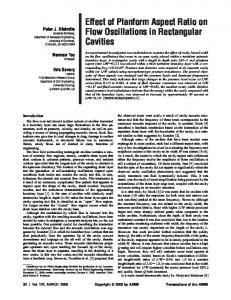
Fig. 6 Profiles of packages used for model validation; „a… validation chip module, „b… 208 pin plastic quad flat pack, „c… cavity up multichip module

Lasance et al. 关9兴 do not discuss the details of their Fourier series model and as a result there may be minor differences between the Lasance model and the model presented herein. Even with the potential for some procedural differences, there is excellent agreement between the two models when calculating mean die temperature over a wide range of boundary conditions, as shown in Table 2. Temmerman et al. 关10兴 tested a 208 pin plastic quad flat pack using several different test procedures, including a submerged double jet impingement test where heat transfer coefficients in excess of 105 W/共m2•K) can be obtained over the entire surface of the package. Other tests were performed using a cold plate on one or both planar surfaces of the package. The plastic quad flat pack, as shown in Fig. 6共b兲, was constructed of plastic mold compound with outside dimensions of 28 mm⫻28 mm, a thermal conductivity of 0.6 W/共m•K兲 and an overall thickness of 3.6 mm. The plastic outer shell fully encapsulated a thermal test die 共SGS-Thomson P655兲 that was 9.1 mm ⫻9.1 mm⫻0.6 mm. The die was made of silicon with a reported thermal conductivity of 155 W/共m•K兲. The test die was attached Table 1 Geometric and thermophysical properties for the validation chip module

The film coefficient in the cavity, h cav is based on the radiative and conductive exchange between the two surfaces while convection is considered to be negligible. h cav⫽h rad⫹h cond

(58)

Model Comparison Lasance et al. 关9兴 designed a hypothetical validation chip module to be used as a benchmark in a study of thermal characterization of electronic packages using a commercially available numerical simulation code. The idealized package with overall dimensions of 30 mm⫻30 mm dissipated 1 W over a die 3 mm ⫻3 mm and consisted of four homogeneous layers as shown in Fig. 6共a兲, where the dimensions and thermal conductivities are listed in Table 1. The geometry of their idealized package was simple enough that Lasance et al. used a conventional Fourier series solution for stacked laminates to obtain the mean temperature of the heat source. Although Lasance’s data do not provide a validation for the more complicated geometries found in most electronic packages, they do provide a convenient benchmark for the fundamental multilayer solution presented in this paper. Journal of Electronic Packaging

Table 2 Comparison of junction temperatures between Lasance et al. †9‡ and current model

SEPTEMBER 2000, Vol. 122 Õ 237

Table 3 Comparison of junction to case resistance between Temmerman et al. †10‡ and the current model

to a heat spreader with a thermal conductivity of 300 W/共m•K兲 and a thickness of 0.13 mm using a die attach material with a thermal conductivity of 2.5 W/共m•K兲 and a mean thickness of 0.005 mm. The heat spreader was then attached to the leadframe with 52 pins per side with a pitch of 0.5 mm. All testing was performed with a total power input of 1 W. Thermal resistance values were calculated based on measured values of the steady state power dissipation, the junction temperature and a reference temperature based on the cold plates, the fluid or the ambient conditions. The difference between the experimental data and the Fourier series model is less that ⫹7.5 percent for each of the three test procedures as shown in Table 3. No explanation is offered by Temmerman for the identical junction to case resistance when the heat transfer coefficient of the top surface changes from 20 to 40 W/共m2•K兲. The Fourier series model exhibits sensitivity to the change in the heat transfer coefficient and the resulting thermal resistance for the higher heat transfer coefficient is lower by 6.6 percent. Sullhan et al. 关8兴 examined several different types of packages, including pin grid arrays with single dies and multichip modules with five dies in both cavity up and cavity down configurations. The cavity up multichip module 共MCM兲 examined by Sullhan et al. 关8兴 had a cross sectional profile as shown in Fig. 6共c兲. The substrate of the package consisted of a three layer stack, with the first layer made of alumina, the second was a leadframe layer made of kovar and finally a die attach layer of silver filled epoxy. For modeling purposes, the silicon dies were assumed to be infinitely thin with a uniform heat flux distribution. The seal ring or sidewalls of the MCM were designed to be a primary conductive path for heat dissipation to the aluminum heat sink attached to the seal lid of the package. The seal ring and seal lid were constructed from a copper tungsten alloy and molybdenum, respectively. The dimensions and the thermal conductivity of each of the materials used in the MCM are given in Table 4. Sullhan et al. 关8兴 did not explicitly give the thermal resistance of their extruded aluminum

Table 4 Thicknesses and thermal conductivities used in the cavity up multichip module

Table 5 Data for dies in multichip modules

heat sink but representative values for R ␪ ja with an approach velocity of 1.5 m/s and a 50 mm⫻50 mm⫻12.5 mm heat sink are in the range of 2.1 to 2.8°C/W. For modeling purposes a value of R ␪ ja ⫽2.5°C/W has been selected. A thermal grease was used between the heat sink and the seal lid to minimize the contact resistance and to promote heat transfer to the heat sink. The MCM had 5 dies of various sizes and power levels as shown in Table 5. All exposed surfaces of the MCM are assumed to have a uniformly specified convective boundary condition. An approach velocity of 1.5 m/s 共300 fpm兲 is used. The heat transfer coefficient is based on a formulation given by Sullhan et al., such that: h⫽2⫻0.000546⫻ 冑V/L

(59)

where V, the velocity is in fpm, the flow length, L is given in inches and the resulting heat transfer coefficient has units of W/共in.2•°C兲. The MCM is attached to an FR-4 printed circuit board through the kovar leads. A lead conductance of 3400 W/共m2•K兲 was used for modeling based on a pin length of 4.57 mm (substrate⫹package standoff) and a pin conductivity of 15.57 W/共m•K兲. The calculated die temperatures, as shown in Table 5, compare favorably with the measured die temperatures reported by Sullhan et al. The hottest die temperature differs from experimental measurements by 4.2 percent. Die 4 and die 5 are the same size and dissipate the same power. Normally one would expect die 5 to be the cooler of the two because it is located in the corner of the MCM and benefits from cooling to two adjoining sides. The model shows this trend; however, the experimental data show just the opposite.

Conclusions The complex geometries found in most electronic package configurations can be modeled using analytical methods through the careful use of simplifying assumptions. The Fourier series solution presented here provides a method for calculating local temperature distributions, heat fluxes and thermal resistances with an accuracy of approximately ⫾5 percent using a fraction of the setup and simulation time expected with more traditional domain discretization procedures.

Acknowledgments The authors acknowledge would like to acknowledge the financial support of the Materials and Manufacturing Ontario and R-Theta Inc., Mississauga, ON.

Nomenclature a,b A A Bi 238 Õ Vol. 122, SEPTEMBER 2000

⫽ ⫽ ⫽ ⫽

Fourier coefficients surface area of the body, m2 coefficient matrix Biot number Transactions of the ASME

f,g h i j k L1 L2 M1 M2 M3 N t T u x,y,z X(x) Y (y) Z(z) wj

⫽ ⫽ ⫽ ⫽ ⫽ ⫽ ⫽ ⫽ ⫽ ⫽ ⫽ ⫽ ⫽ ⫽ ⫽ ⫽ ⫽ ⫽ ⫽

explicit constants found in Eqs. 共20兲 and 共21兲 heat transfer coefficient, W/共m2•K兲 layer identification die plane section identification thermal conductivity, W/共m•K兲 package length, m package width, m top layer in basecell 共die plane layer兲 top layer in sidewall sections bottom layer in package cap series truncation limit layer thickness; m temperature; °C solution vector Cartesian coordinates, m separation function separation function separation function sidewall widths, m

Subscripts a bot cap cav cond die rad s

⫽ ⫽ ⫽ ⫽ ⫽ ⫽ ⫽ ⫽

ambient bottom surface cap cavity conduction die radiation sidewall sections

Greek Symbols

⑀ ⫽ characteristic root for x-direction ␥ ⫽ composite characteristic root ␭ ⫽ characteristic root for x-direction

Journal of Electronic Packaging

␬ i ⫽ conductivity ratio; ⬅k i /k i⫹1 ␪ ⫽ temperature rise, °C ⌰ ⫽ sidewall temperature difference as in Eqs. 共18兲 and 共24兲

References 关1兴 Gray, P. R., 1971, ‘‘Analysis of Electrothermal Integrated Circuits,’’ IEEE J. Solid-State Circuits, SC-6, No. 1, pp. 8–14. 关2兴 Kokkas, A. G., 1974, ‘‘Thermal Analysis of Multiple-Layer Structures,’’ IEEE Trans. Electron Devices, ED-21, No. 11, pp. 674–681. 关3兴 Lemczyk, T. F., Culham, J. R., and Yovanovich, M. M., 1989, ‘‘Analysis of Three-Dimensional Conjugate Heat Transfer Problems in Microelectronics,’’ Numerical Methods in Thermal Problems, Proceedings of the Sixth International Conference, Swansea, U.K., pp. 1346–1356. 关4兴 Carslaw, H. S., and Jaeger, J. C., 1959, Conduction of Heat in Solids, Second Edition, Oxford University Press, Oxford. 关5兴 Albers, J., 1994, ‘‘An Exact Recursion Relation Solution for the Steady-State Surface Temperature of a General Multilayer Structure,’’ Proceedings of the 10th IEEE Semiconductor Thermal Measurement and Management Symposium, Austin, TX, pp. 129–137. 关6兴 Lemczyk, T. F., and Culham, J. R., 1992, ‘‘Thermal Analysis of Electronic Package Components,’’ Microelectronics Heat Transfer Laboratory Report, UW/MHTL 9112 G-37, University of Waterloo, Waterloo, Canada, April, 1992. 关7兴 Kelman, R. B., 1979, ‘‘Least Squares Fourier Series Solutions To Boundary Value Problems,’’ SIAM Rev., 21, No. 3. 关8兴 Sullhan, R., Fredholm, M., Monaghan, T., Agarwall, A., and Kozarek, B., 1991, ‘‘Thermal Modeling and Analysis of Pin Grid Arrays and Multichip Modules,’’ Proceedings of the 7th IEEE Semiconductor Thermal Measurement and Management Symposium, Phoenix, AZ, pp. 110–116. 关9兴 Lasance, C., Vinke, H., Rosten, H., and Weiner, K., 1995, ‘‘A Novel Approach for the Thermal Characterization of Electronic Parts,’’ Proceedings of the Eleventh Annual IEEE Semiconductor Thermal Measurement and Management Symposium, San Jose, CA, pp. 1–9. 关10兴 Temmerman, W., Nelemans, W., Goossens, T., Lauwers, E., Lacaze, C., and Zemlianoy, P., 1995, ‘‘Validation of Thermal Models for Electronic Components,’’ Proceedings of the Technical Conference, International Electronics Packaging Conference, San Diego, CA, pp. 142–150. 关11兴 Bar-Cohen, A., 1994, ‘‘Trends in the Packaging of Computer Systems,’’ Cooling of Electronic Systems, S. Kakac, H. Yuncu, and K. Hijikata, eds., Series E: Applied Sciences-Vol. 258, Kluwer Academic Publishers, Norwell, MA.

SEPTEMBER 2000, Vol. 122 Õ 239