Using ASME format

Josette Devaux Ge´rard Mottet Jean-Michel Bergheau1 Systus International 69485 Lyon Cedex 03, France

Surender K. Bhandari Framatome, Tour Framatome, 92084 Paris La De´fense Cedex, France

Claude Faidy

Evaluation of the Integrity of PWR Bimetallic Welds This paper presents the state of the art and the progress made in the numerical simulation of the stress state in a complex multi-material structure, using not only sophisticated finite element tools, but also the simplified engineering methods. A comparison of the numerical results concerning residual stresses is made with those measured using X-ray diffraction method and incremental hole-drilling technique. Finally, an example is given on the analysis of a fully circumferential crack in a typical bimetallic weld under pressure, thermal, and residual stresses. 关S0094-9930共00兲00703-4兴

EDF/SEPTEN, 69628 Villeurbanne, France

1

Introduction

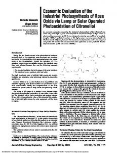
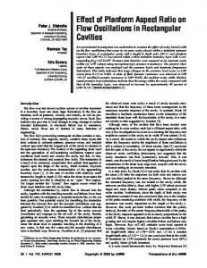
The junction of an austenitic primary pipe on a ferritic vessel nozzle needs a special manufacturing procedure. This procedure concerns the fabrication of a bimetallic weld. The nozzle end has an austenitic steel buttering and safe-end that can be welded easily to the austenitic pipework to ensure a good final junction 共Fig. 1兲. Superficial defects can appear in the weld buttering during the work in service. The origin of such defects probably comes from an oxidation mechanism at the grain boundaries due to the different heat treatments applied to the bimetallic junction. The complete analysis of the behavior of such a defect needs a priori to take account of the metallurgical and mechanical consequences induced by the manufacturing procedure. Indeed, welding and cladding operations lead to complex changes in the microstructure and to generation of residual stresses, the role of which can be very important for the propagation of defects. In this paper, we present the finite element simulation of the behavior of such a junction. The analysis is performed in two steps: • numerical simulation of the manufacturing sequence, including internal cladding, final stress relieving heat treatment, and hydrotest; • numerical study of the behavior of a superficial circumferential defect in the case of a severe accident loading. Two simulations have been achieved to get the residual stress state after the final stress relieving heat treatment. The first one takes account of the interactions between heat transfer, metallurgy, and mechanics which take place during the different stages of the manufacturing procedure. The second one assumes that stresses completely relax during the final stress-relieving heat treatment so that remaining residual stresses are due only to the difference between the heat expansion coefficients during the final cooling. The results of both simulations are discussed and compared to experimental measurements using the X-ray diffraction method and the incremental hole-drilling technique. The behavior of a defect, which is assumed to appear during the normal operation, is analyzed using the numerical results of the manufacturing procedure 共residual stresses and microstructure兲. We postulate the presence of a fully circumferential crack located 1 Now with LTDS, UMR 5513 CNRS/ECL/ENISE, 58 Rue J. Parot, 42023 St Etienne Cedex 2, France. Contributed by the Pressure Vessels and Piping Division for publication in the JOURNAL OF PRESSURE VESSEL TECHNOLOGY. Manuscript received by the PVP Division, February 1, 2000; revised manuscript received April 5, 2000. Technical Editor: S. Y. Zamrik.

368 Õ Vol. 122, AUGUST 2000

in the buttering at 200 ␮m from the interface, emerging on the outer surface and of depth 8 mm 共Figs. 1 and 3兲. This choice will be justified by the results of the simulation of the manufacturing procedure. The aim of this study is to demonstrate that such crack, if it exists, remains stable 共i.e., does not propagate兲 under normal operating as well as accidental conditions, such as the one encountered in LOCA conditions 共loss of coolant accident兲 corresponding to the failure of a primary pipe. One can note that because the postulated crack is assumed to be fully circumferential, the studied configuration corresponds to an extremely penalizing situation.

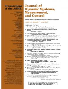
2 Assessment of the Residual Stress State due to Manufacturing 2.1 Complete Modeling of the Manufacturing Procedure. The simulation of the manufacturing procedure takes account of the complex interactions between heat transfer, metallurgy, and mechanics as shown in Fig. 2, and has been achieved using the finite element software SYSWELD® 关1,2兴. All the calculations are performed under axisymmetric conditions and the mesh used 共Fig. 3兲 contains 1417 second-order reduced integration elements 共8 and 6-node elements兲 and 3708 nodes. One can note that the defect is included in the mesh. This has been done in order to use the same mesh for the simulation of the manufacturing procedure and the analysis of the behavior of the defect, and thus, to avoid any numerical error coming from the

Fig. 1 Typical bi-metallic joint

Copyright © 2000 by ASME

Transactions of the ASME

Downloaded 10 Feb 2009 to 193.50.200.66. Redistribution subject to ASME license or copyright; see http://www.asme.org/terms/Terms_Use.cfm

mations between phases. In the present calculation, the following phase transformations of A508Cl3 steel have been taken into account: • base metal 共tempered bainite兲→austenite • austenite→as-quenched bainite • austenite→as-quenched martensite

Fig. 2 Interactions between physical phenomena „couplings indicated with a dotted line are neglected…

The modeling of tempering is very important because it results in a reduction of the yield stress of the material. In the present calculation, tempering phenomena are schematized as special transformations from some as-quenched structure to some totally tempered one. Partially tempered structures are represented by mixtures between as-quenched and completely tempered structures. Therefore, two special transformations have been introduced in the model: • as-quenched bainite→totally tempered bainite • as-quenched martensite→totally tempered martensite. Thermal Analysis. The thermal analysis rests upon the classical heat equation with associated boundary conditions. The present calculation is nonlinear, i.e., the heat capacity and thermal conductivity depend on temperature and nonlinear boundary conditions are included in the model. The thermal and metallurgical calculations are fully coupled because thermal properties are phase-dependent and metallurgical transformations are accompanied by latent heat effects, which modify the temperature distribution. Therefore, the thermal conductivity ␭, the density ␳ and the enthalpy H are approximated by linear mixture laws from the thermal properties of each phase 共␳ k being the proportion of phase k兲 ␭共 pk ,␪ 兲⫽

␳共 pk ,␪ 兲⫽ H共 pk ,␪ 兲⫽

Fig. 3 Mesh „1417 elements, 3708 nodes…—manufacturing procedure—defect location

transfer of the results from one mesh to another. Of course, during the manufacturing sequence, the defect is maintained closed using two-node special elements. 2.1.1 Software Capabilities Metallurgy. As far as ferritic steels are involved, metallurgy must be included in the simulation. Different approaches can be used for the modeling of transformation kinetics in steels. The model used for the present simulation rests upon the following simple kinetic equation 关3兴 in the case of one transformation between two phases 共p denoting the proportion of formed phase兲: p˙ ⫽

¯p 共 ␪ 兲 ⫺p f 共 ␪˙ 兲 ␶共 ␪ 兲

(1)

where ¯p ( ␪ ) represents the phase proportion obtained after an infinite time at temperature ␪ and ␶共␪兲, a time delay. This equation is used to describe diffusion-controlled as well as martensitic transformations. In the latter case, the function f ( ␪˙ )⫽⫺ ␪˙ such that martensitic transformation only depends on temperature. This model has been generalized in order to deal with several transforJournal of Pressure Vessel Technology

兺

p k␭ k共 ␪ 兲

(2a)

兺

p k␳ k共 ␪ 兲

(2b)

兺

p kH k共 ␪ 兲

(2c)

phases

phases

phases

One can note that Eq. 共2c兲 includes latent heat effects since the H k ( ␪ ) reflect both thermal inertia effects of the phases and the latent heat of transformation between the latter. The detailed physical phenomena occurring in the electric arc are not included in the model. The welding arc is simply represented by a suitable heat source, the dimensions and power of which are calibrated on an experimental heat-affected zone. Mechanical Analysis. The interactions between thermal and mechanical analyses come from dilatation effects and the temperature dependency of the stress-strain relation. Plastic dissipation is neglected due to the relative small strains encountered in welding applications 关4兴. Metallurgy is involved in the mechanical analysis through four effects: 1 the volume changes resulting from transformations, 2 the phase and temperature dependency of the constitutive equations of the material, 3 the transformation plasticity behavior, 4 the effect of mechanical parameters 共stresses and strains兲 on metallurgical transformations. Volume changes arising from transformations widely contribute to the generation of residual stresses and strains. These changes are accounted for by replacing the classical thermal strain by some ‘‘thermometallurgical’’ one ␧ th共 ␪ 兲 ⫽

兺

Phases

p k ␧ th k 共␪兲

(3)

AUGUST 2000, Vol. 122 Õ 369


where the ␧ th k reflect both the thermal strain of the phases and the volume changes between the latter 关5兴. The stress-strain relation must be temperature-dependent, representative of the phase mix, and reproduce the transformation plasticity phenomenon. The steel behavior during transformation is usually supposed to be elastoplastic. Viscoplastic 共timedependent兲 effects are neglected except of course for stress relieving heat treatments. The elastic behavior is supposed to be the same for all the phases. The plastic strain rate ( ␧˙ p ) can be decomposed as the sum ˙ ), the of three terms 关5兴, proportional to the stress variation ( ␴ ˙ temperature variation ( ␪ ), and phase proportion variation (p˙ ), respectively, (4) The first two terms of Eq. 共4兲 represent the classical plastic strain rate ( ␧˙ c p ), while the third one represents transformation-induced plastic strain rate ( ␧˙ t p ). Transformation plasticity describes the plastic flow resulting from a variation of the phase proportions that occurs even for very small applied stresses. Transformation plasticity, in A508 Cl3, mainly arises from the Greenwood-Johnson mechanism 关6兴 that assumes that microscopic plasticity is induced in the austenitic phase by volume variations between the phases and is oriented in the load direction. The complete model implemented in SYSWELD® and used for the present calculation is based on both theoretical and numerical studies 关5,7–9兴. Strain-hardening phenomena are included in the formulation 关8兴 as well as the memory or recovery of hardening during transformations. As mentioned previously, viscoplastic effects are neglected in the welding simulations but they are taken into account in simulations of stress relieving heat treatments. The model used is described in details in 关10兴. The effect of mechanical parameters on metallurgical transformations is neglected in the present simulation due to the lack of experimental data. Material Data. The material data used for the thermal, metallurgical and mechanical calculations are reported in 关11兴. Calculation Procedure. The finite element simulation of each stage of the manufacturing procedure, involving the interactions between heat transfer, metallurgy, and mechanics, is performed in two steps. First, a fully coupled thermal and metallurgical analysis is performed in order to compute the temperature at all the nodes of the mesh and the phase proportions in the elements. Then, the mechanical calculation uses these results to calculate the residual stress distribution and the distortion of the structure. 2.1.2 Description of the Manufacturing Sequence and Modeling Conditions. The manufacturing sequence of a bimetallic junction consists of six main stages 共Fig. 3兲. 1st Stage: Buttering of the Nozzle Face. This operation is achieved in three steps. A first layer of buttering, made of 309L austenitic steel, followed by another deposit in 308L austenitic steel are first realized using a coated electrode process, the structure being preheated to 125–150°C. A stress-relieving heat treatment at 550°C during 2 h is then applied. The last sequence of buttering is then performed using several layers of 308L coated electrode process again. From the modeling point of view, we suppose that the stress relieving heat treatment leads to total relaxation of stresses at high temperature. Therefore, the first operation simulated consists of cooling from 550°C to ambient temperature, the induced stresses coming from the difference between the heat expansion coefficients of the different materials. Because of the large amount of calculation implied by the complete simulation of the deposition of all the weld beads, the last sequence of buttering is simulated using a ‘‘macrobeads’’ technique. This technique consists in gathering the weld beads in groups, called macrobeads. Then we im370 Õ Vol. 122, AUGUST 2000

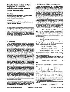
pose on each macrobead, the thermal cycle corresponding to an individual weld bead. Here, only one macrobead is used. 2nd Stage: Assembling of the Nozzle Face. This operation is achieved in three sequences. The first sequence concerns the filling of one third of the chamfer with 308L austenitic steel. The first root beads inside the nozzle are then removed and new weld beads are deposited starting from inside the nozzle 共back weld兲. At last, the filling of the chamfer is completed. The welding process employed here is either a submerged arc welding or a coated electrode process. The modeling uses again the ‘‘macrobeads’’ technique introduced previously. The filling of one third of the chamfer is realized in one macrobead as well as the back weld. The final filling of the chamfer is achieved using seven macrobeads. The nearer the macrobead is to the outer surface, the smaller it is considered. In order to calculate accurately the residual stresses in the outer surface, the thickness of the three last macrobeads 共4 mm兲 corresponds approximately to the thickness of one layer of weld beads. 3rd Stage: Machining of the External Diameter 共Slope 5 deg兲. This operation is simulated by making the mechanical properties vanish in the finite elements located in the oversize zone indicated in Fig. 3. 4th Stage: Deposition of the Internal Cladding in Two Layers Using the Strip Cladding Process. The first layer, made in 309L, is deposited with a preheating at 150°C. The second layer, in 308L, is realized at ambient temperature. Here again, the macrobeads technique is used for the calculation, only one macrobead being used for each layer. 5th Stage: Intermediate Postweld Heat Treatments and Final Stress Relieving Heat Treatment. The nozzle is then welded on the vessel and intermediate postweld heat treatments are applied to the whole structure at 550°C during 4 h. A heat treatment being applied to a pair of nozzle assemblies 共except the last two兲 and the vessel comprising eight nozzles, each nozzle can be submitted up to three intermediate heat treatments. A final stress-relieving heat treatment at 610°C during 15 h, with a holding at maximal temperature during 6 h at least, is then applied. The cooling at ambient temperature is realized in such a way that no temperature gradient takes place in the structure. From the modeling point of view, only the final heat treatment has been simulated because it is the most significant. The modeling of the stress relief is here achieved as accurately as possible. Of course, stress relaxation is taken into account through the use of a suitable elastic-viscoplastic model. But, in the case of A508Cl3, tempering effects are also accounted for and the elasticviscoplastic behavior depends on the metallurgical phase proportions calculated during the previous manufacturing stages. 6th Stage: Hydrotest. Finally, the nozzle is submitted to a hydrotest at 22.8 MPa 共1.33 times the reference pressure兲. This operation is simply simulated by applying an internal pressure. 2.2 Simplified Simulation. For this calculation, we suppose that the stresses vanish at the end of the holding time at 610°C during the final stress-relieving heat treatment. Starting from a uniform temperature 共610°C兲 in all the materials, the structure is cooled to ambient temperature. Therefore, manufacturing residual stresses only arise from the differences between the heat expansion coefficients of the materials. The same material data 关11兴 and mesh 共Fig. 3兲 are used for the simulation, but here the materials are supposed to be in their initial state. 2.3 Results and Discussion. Figures 4 and 5 give the longitudinal and hoop stress contours, respectively. The computed distributions of the longitudinal stress are different 共Fig. 4兲. The simplified calculation gives a bending stress in the ferritic zone; compressive longitudinal stresses are computed just below the claddings and tensile stresses are calculated on the outer surface. By contrast, the complete simulation gives a maximum compressive stress in the middle of the thickness and quasi-zero stresses Transactions of the ASME


Fig. 4 Longitudinal stress contours „top: complete simulation; bottom: simplified simulation…

agreement with experimental measurements. Nevertheless, the stress at the interface is slightly overestimated with the simplified calculation 共630 instead of 530 MPa for the complete simulation兲. More important differences are obtained for the residual hoop stress. The simplified calculation leads to higher stress values both on the ferritic and the austenitic sides. At the interface, the simplified simulation gives 325 MPa, while the complete simulation only gives 175 MPa. One can note that the hoop stresses calculated by the complete simulation are in very good agreement with the experimental measurements. As a conclusion, one can say that, except for the longitudinal stress on the outer surface near the interface, the stresses computed by the simplified and complete simulations are different. It is therefore important to simulate the deposition of the internal cladding in order to estimate the stresses on the inner side. In the same way, the computation of residual stresses in the austenitic safe-end needs the modeling of the filling of the chamfer. However, if one is only interested in the longitudinal peak stress on the outer surface, then the simplified approach seems to be sufficient. Moreover, this stress peak is somewhat overestimated, which can enable some conservative analysis of the behavior of some defect located at the interface on the outer surface.

Fig. 5 Hoop stress contours „top: complete simulation; bottom: simplified simulation…

below the claddings. The maximum longitudinal stress computed by both simulations is equivalent and is located on the outer surface at the interface between austenitic and ferritic steels. Looking at the results along the interface between both materials, one can note that important tensile longitudinal stresses are computed on the outer side. This explains the position of the defect which will be studied in the second part of this paper, the defect being located in the austenitic zone 共at 200 ␮m from the interface兲 on the outer surface, due to sensitivity of austenitic steel heat-affected zone to oxidation-induced cracking mechanism. On the austenitic safe-end side, both simulations give small longitudinal stresses. The simplified and complete simulations give different hoop stress distributions 共Fig. 5兲. Inside the austenitic safe-end and the weld, the complete simulation gives stresses that may reach 700 MPa, while the maximum hoop stress computed by the simplified simulation is about 250 MPa in the middle of the thickness on the buttering side. Moreover, the complete simulation gives compressive hoop stresses on the surface of the weld, while the simplified simulation gives small tensile stresses. Experimental measurements of the residual stress state have been achieved using the X-ray diffraction method and the incremental hole-drilling technique 关12兴. The residual longitudinal and hoop stresses computed by both simulations are compared with experimental measurements along the outer surface near the interface between austenitic and ferritic steels in Figs. 6 and 7, respectively. The longitudinal stress profiles computed by both simulations are quite similar and in good Journal of Pressure Vessel Technology

Fig. 6 Comparison between computed and measured longitudinal stresses along the outer surface

Fig. 7 Comparison between computed and measured hoop stresses along the outer surface

AUGUST 2000, Vol. 122 Õ 371


3

Behavior of a Defect in Case of Severe Loading

This section presents the behavior of a fully circumferential crack of depth 8 mm on the outer surface in the buttering at 200 ␮m from the interface, and subjected to a severe accidental loading. 3.1 Description of the Loading. The loading is applied in 3 stages. 1st Stage: Opening of the Defect Under Residual Stresses. Starting from the results of the complete simulation of the manufacturing procedure, the defect integrated in the mesh, which was maintained closed up to this point, is now opened. This crack opening is possible because the manufacturing worksheet has led to tensile residual longitudinal stresses near the defect. In order to represent the influence of primary piping that is not schematized here, we assume the end of the cap to remain plane; this corresponds to a penalizing loading situation. These conditions are applied for all the stages. 2nd Stage: Cycling Between Nominal Operation and Shut Down. The rising to nominal operation is characterized by the following conditions. A heating rate from ambient temperature to 323°C 共primary fluid temperature at the vessel outlet兲 is imposed at the whole structure. We suppose that the temperature rate is sufficiently slow so that no temperature gradient takes place in the structure. In parallel, an internal pressure 共15.5 MPa兲 is applied to the nozzle. The effect of pipe expansion is represented by a longitudinal force equal to ⫺18.7 104 N and a bending moment equal to 208 104 m.N applied to the end of the cap. Due to the axisymmetric modeling used, the loading corresponding to the maximal tensile force induced by the bending moment is considered. After a first rising to the nominal operating conditions, a shutdown and a second rising to nominal operation is simulated. The corresponding evolutions of temperature and pressure are defined according to a fictitious time and given in Fig. 8. The fictitious time equal to 1 corresponds to the opening of the defect, times 4 and 8 to nominal operating conditions, and time 5 to the shutdown. 3rd Stage: Loading Corresponding to LOCA Conditions. A sudden decrease in the internal pressure 共from 15.5 MPa to 0.1 MPa in 20 s兲 and a decrease of the primary fluid temperature characterize the LOCA situation. But the most critical situation corresponds to the peak of both the longitudinal force 共1244 104 N兲 and the bending moment 共247 104 m.N兲 due to the rupture of pipes, which happens 1 s after the beginning of LOCA. Therefore, only this force peak is analyzed, the temperature as well as the pressure being supposed not to have changed during the first second. The LOCA simulation is associated with the fictitious time equal to 9 共Fig. 8兲.

steel of the buttering兲. Experimental investigations have shown that, in such situations, the apparent toughness of welded bimetallic junctions depend on the differences between the hardness of the materials on each side of the interface. For experiments performed at a temperature above the brittleductile transition of the ferritic part of a bimetallic weld, rupture mostly comes from tearing of the austenitic steel that has a lower yield stress. It is well known that ductile tearing strongly depends on the stress triaxiality ratio 关13兴. It is therefore expected that the overall toughness of bimetallic welds depends on the way the harder ferritic steel limits the development of plastic strain in the weaker austenitic steel and how this affects the stress triaxiality. Starting from the toughness of a homogeneous material, it is therefore possible to assess the toughness of the same material in a nonhomogeneous situation using elastic-plastic finite element simulation and local approach of ductile tearing 关14兴. The damage criterion 关15兴 used for this study relates the average growth of cavities initiated around inclusions to both the average plastic strain and the stress triaxiality ratio in the finite elements located at the crack tip

冉冊

冉冊

d R 3 ␴m p ln ⫽0.28 exp ␧˙ dt R0 2 ␴ eq eq

(5)

In Eq. 共5兲, R and R 0 are the actual and initial mean cavity radius, ␴ m is the mean stress, ␴ eq the von Mises equivalent stress p 共␴ m / ␴ eq is the stress triaxiality ratio兲, and ␧˙ eq the equivalent plastic strain rate. The size (I c ) 3 of the finite elements at the crack tip is related to the microstructure and is defined in order to ensure a physical meaning to continuum mechanics. Usually, I c is chosen such that (I c ) 3 contains about eight inclusions and in the present case, I c ⫽200 ␮ m. Equation 共5兲 is integrated with respect to time using the results of an elastic-plastic simulation. Tearing is supposed to occur when R/R 0 reaches some critical value (R/R 0 ) c corresponding to coalescence of cavities. (R/R 0 ) c is determined according to the experimental toughness of the homogeneous material using the elastic-plastic simulation of a homogeneous austenitic CT50 specimen. Then this tearing criterion is applied to the multi-material CT50 specimen corresponding to the situation encountered with the bimetallic weld 共Fig. 9兲 in order to determine the corresponding toughness.

3.2 Assessment of the Apparent Toughness of the Bimetallic Weld. The studied defect is located in the buttering, in the immediate vicinity of a hard heat-affected zone created in the ferritic steel by the first layer of buttering. Therefore, the defect is surrounded by both a hard structure and a softer one 共austenitic

Fig. 8 Pressure and temperature evolutions applied during the three stages of the loading

372 Õ Vol. 122, AUGUST 2000

Fig. 9 Mesh of the multi-material CT50 specimen

Transactions of the ASME


The CT50 specimen simulations are performed under a 2D plane strain assumption and J is calculated from the results of the numerical simulations using the theta method 关16,17兴. Devaux et al. 关14兴 give toughness values at 100°C between 100 and 170 kJ/m2. In order to make conservative studies, a value (R/R 0 ) c ⫽1.64 leading to J Ic ⫽80.5 kJ/m2 is chosen. Assuming that the critical (R/R 0 ) c value is temperature independent, the apparent toughness value predicted from the simulation of the multimaterial CT50 specimen at 323°C corresponding to our case is 32 kJ/m2, while the lowest value experimentally determined is 35 kJ/m2 that validates the proposed methodology. 3.3

Results and Discussion

1st Stage: Opening of the Defect. Figure 10 gives the deformed shape of the defect arising from the residual stress state due to the manufacturing procedure. The relative displacements of the first couple of nodes located on the crack lips starting from the crack tip show that K values in modes I and II are very similar 共Fig. 11兲. The J value calculated using the theta method is 21.3 kJ/m2, which is lower than the apparent toughness of the bimetallic weld. 2nd Stage: Cycling Between Nominal Operation and Shutdown. The relative displacements of the crack lips, reported in Fig. 11, clearly show that the mode II loading still remains important and equivalent to mode I. The J values are reported in Fig. 12 as a function of the fictitious time defined by Fig. 8. One can note that the maximum J value reached remains much less than the toughness of the material.

Fig. 10 Deformed shape of the defect after the opening stage

Fig. 11 Relative displacements of the crack lips „400 ␮m from the crack tip…

Fig. 12

J values for the different loading steps

Journal of Pressure Vessel Technology

3rd Stage: Loading Corresponding to LOCA Conditions. The maximum computed J value in this case turns out to be 17.21 kJ/m2, which again is lower than the toughness of the material. It can therefore be concluded that the defect will remain stable under LOCA conditions as well.

4

Conclusion

The paper deals with the integrity of a typical PWR bimetallic weld. After the evaluation of the residual stress field corresponding to the complete manufacturing sequence, the behavior of a crack is studied under nominal operating as well as accidental conditions. It is concluded that a fully circumferential crack of depth 8 mm, located in the buttering at 200 ␮m from the interface, on the outside surface, will remain stable under an accidental loading condition, LOCA, corresponding to the failure of a primary pipe, analysis being performed considering conservative boundary conditions to represent primary piping and low material toughness.

References 关1兴 Bergheau, J.-M., and Leblond, J.-B., 1991, ‘‘Coupling Between Heat Flow, Metallurgy and Stress-strain Computations in Steels—The Approach Developed in the Computer Code SYSWELD for Welding or Quenching,’’ Modeling of Casting, Welding and Advanced Solidification Processes V, M. Rappaz, M. R. Ozgu, and K. W. Mahin. eds., The Minerals, Metals & Materials Society, pp. 203–210. 关2兴 Leblond J.-B., Pont D., Devaux J., Bru D., and Bergheau J.-M., 1997, ‘‘Metallurgical and Mechanical Consequences of Phase Transformations in Numerical Simulations of Welding Processes,’’ Modeling in Welding, Hot Powder Forming and Casting, Chap. 4, L. Karlsson, ed., ASM International, pp. 61– 89. 关3兴 Leblond, J.-B., and Devaux, J.-C., 1984, ‘‘A New Kinetic Model for Anisothermal Metallurgical Transformations in Steels Including the Effect of Austenit Grain Size,’’ Acta Metall., 32, pp. 137–146. 关4兴 Karlsson L., and Lindgren, L.-E., 1991, ‘‘Combined Heat and Stress-Strain Calculations,’’ Modeling of Casting, Welding and Advanced Solidification Processes V, M. Rappaz, M. R. Ozgu, and K. W. Mahin, eds, The Minerals, Metals & Materials Society, pp. 187–202. 关5兴 Leblond, J.-B., Mottet, G., and Devaux, J.-C., 1986, ‘‘A Theoretical and Numerical Approach to the Plastic Behavior of Steels During Phase Transformations—I: Derivation of General Relations,’’ J. Mech. Phys. Solids, 34, pp. 395–409. 关6兴 Greenwood, G. W., and Johnson, R. H., 1965, ‘‘The Deformation of Metals Under Small Stresses During Phase Transformations,’’ Proc. R. Soc. London, Ser. A, 283, pp. 403–422. 关7兴 Leblond, J.-B., Mottet, G., and Devaux, J.-C., 1986, ‘‘A Theoretical and Numerical Approach to the Plastic Behavior of Steels During Phase Transformations—II: Study of Classical Plasticity for Ideal-Plastic Phases,’’ J. Mech. Phys. Solids, 34, pp. 411–432. 关8兴 Leblond, J.-B., Devaux, J., and Devaux, J.-C., 1989, ‘‘Mathematical Modeling of Transformation Plasticity in Steels—I: Case of Ideal-Plastic Phases,’’ Int. J. Plast., 5, pp. 551–572. 关9兴 Leblond, J.-B., 1989, ‘‘Mathematical Modeling of Transformation Plasticity in Steels—II: Coupling With Strain Hardening Phenomena,’’ Int. J. Plast., 5, pp. 573–591. 关10兴 Leblond, J.-B., 1989, ‘‘Simulation nume´rique du soudage—Mode`le de viscoplasticite,’’ FRAMASOFT Internal Report, CSS.L.NT.89/4015. 关11兴 Bru, D., 1993, ‘‘Analyze du comportement d’un de˙faut exte´rieur situe˙ dans le beurrage d’une liaison bime´tallique—Rapport A: Pre´sentation des travauxAnnexe 1: caracte´ristiques physiques des mate´riaux utilise´es dans les simulations nume´riques,’’ FRAMASOFT⫹CSI Internal Report, LESW93/2015. 关12兴 Todeschini, P., 1992, ‘‘Mesures de contraintes par diffraction de rayons X en peau externe de la jonctioa`n bi-me´tallique de la tubulure de cuve REP H2 de IRAN 1’’, EDF Internal note HT-41/NEQ 1368-A, EDF-DER Renardie`res, France, Apr. 关13兴 Pineau, A., 1981, ‘‘Review of Fracture Micromechanisms and a Local Approach to Predicting Crack Resistance in Low Strength Steels,’’ Advances in Fracture Research, ICF5, Pergamon, Vol. 2, pp. 553–580. 关14兴 Devaux, J. C., Mottet, G., Houssin, B., and Pelissier Tanon, A., 1987, ‘‘Prediction of Overall Toughness of Bimetallic Welds Through Numerical Analysis According to the Local Approach of Tearing Fracture,’’ Numerical Methods in Fracture Mechanics, A. R. Luxmoore, D. R. J. Owen, Y. P. S. Rajapakse, and M. F. Kanninen, eds., Pineridge Press, pp. 325–335. 关15兴 Rice, J. R., and Tracey, D. M., 1969, ‘‘On the Ductile Enlargement of Voids in Triaxial Stress Fields,’’ J. Mech. Phys. Solids, 17, p. 201. 关16兴 Destuynder, Ph., and Djoua, M., 1981, ‘‘Sur une interpre´tation mathe´matique de l’inte´grale de Rice en the´orie de la rupture fragile,’’ Math. Methods Appl. Sci., 3, pp. 70–87. 关17兴 Gilles, Ph., Mourgue, Ph., Lienard, C., and Bois, C., 1992, ‘‘Efficiency and Accuracy of the G- ␪ Domain Integral for Elasto-Plastic Crack Driving Force Computations,’’ Proc., ICCES’92.

AUGUST 2000, Vol. 122 Õ 373


Using ASME format

Using ASME format

Suggest Documents