eigenvalues for controller designs in Yang and Mote 1. The behavior of closed-loop eigenvalues for the companion problem of a controlled translating beam has ...
W. D. Zhu Assistant Professor, University of Maryland Baltimore County, Baltimore, MD 21250 MEM. ASME
B. Z. Guo Beijing Institute of Technology, Beijing, China
C. D. Mote, Jr. President, (Glenn L. Martin Institute Professor of Engineering) University of Maryland, College Park, MD 20742 Honorary MEM. ASME
1
Stabilization of a Translating Tensioned Beam Through a Pointwise Control Force A spectral analysis determining asymptotically the distribution of eigenvalues of a constrained, translating, tensioned beam in closed form is the subject of this paper. The constraint is modeled by a spring-mass-dashpot subsystem that is located at any position within the span of the beam. It can represent a feedback controller with a collocated sensor and actuator. The necessary and sufficient condition that ensures a uniform stability margin for all the modes of vibration is determined. Influences of system parameters on the distribution of eigenvalues are identified. The analytical predictions are validated by numerical analyses. The constraint location maximizing the stability margin of the distributed model is predicted through a combined analytical and numerical approach. The implications and utility of the results are illustrated. The methodology developed can be extended to predict stability margins and optimize control parameters for controlled translating beams with other types of boundary conditions and controller structures. 关S0022-0434共00兲00702-4兴
Introduction
Translating media model high-speed magnetic tapes, band saws, conveyer belts, transmission chains, tramway cables, textile fibers, webs, paper sheets, and like processes. The quest for ever higher stable speeds of transport to increase productivity is often constrained by transverse vibration of the medium that degrades product or process performance and can even cause system failure. Active control of vibration of translating media can increase the productivity and operating speed limit for many industrial applications. Control methods including domain control 关1,2兴, parametric control, such as control of tension in a string and beam 关3,4兴, and boundary control 关5兴 have been investigated. Control of translating media through domain sensing and actuation provides an effective means to suppress deleterious vibration. It is easy to implement and maintains almost constant tension required in most applications. A translating medium is a distributed gyroscopic system. Control of a finite number of the lower modes can lead to destabilization of uncontrolled higher modes via spillover. Through a transfer function formulation and a root locus method, Yang and Mote 关1兴 first designed pointwise controllers for a translating string that ensure that all the eigenvalues of the controlled system lie strictly within the left-half plane. The method has been successfully implemented on band saws 关6兴 and chain drives 关7兴. However, two fundamental questions remain unknown. The first concerns the margin of stability of the controlled system, namely, the distances of closed-loop eigenvalues from the imaginary axis. With the stability margin defined as the minimum distance over all closed-loop eigenvalues to the imaginary axis, the necessary and sufficient condition for the control parameters, that ensures a nonvanishing, uniform stability margin for all the modes of vibration, has not been determined. This condition can ensure exponential rates of decay of the energy of vibration of distributed translating media. If the stability margin vanishes, the energy of vibration decays only asymptotically. Second, the optimal control parameters leading to maximal rates of decay of the energy of vibration of distributed translating media have not been investiContributed by the Dynamic Systems and Control Division for publication in the JOURNAL OF DYNAMIC SYSTEMS, MEASUREMENT, AND CONTROL. Manuscript received by the Dynamic Systems and Control Division September 9, 1998. Associate Technical Editor: N. Olgac.
322 Õ Vol. 122, JUNE 2000
gated. They are useful in applications where stabilization of a largest number of modes at the fastest rate is necessary. Translating media are typically modeled as a translating string or tensioned Euler–Bernoulli beam. A translating string under control by a point force is asymptotically stable only when the dimensionless location of the control device is an irrational number 关1,8兴. Any rational number corresponds to a nodal point of vibration of the uniform translating string. Though all the eigenvalues of a controlled translating string remain strictly in the lefthalf plane, an infinite number of them approach the imaginary axis 关8兴. The energy of vibration of the system decays asymptotically, but not exponentially. The spectral analysis developed in Zhu et al. 关8兴 can be used to predict the locations of closed-loop eigenvalues for controller designs in Yang and Mote 关1兴. The behavior of closed-loop eigenvalues for the companion problem of a controlled translating beam has not been reported in the literature. The purposes of this paper are twofold. First, the asymptotic distribution of eigenvalues of a controlled translating beam is investigated. The necessary and sufficient condition ensuring a uniform stability margin for all the modes of vibration is identified. To demonstrate the methodology, a translating tensioned beam with mixed boundary conditions, under a pointwise constraint modeled by a mass-spring-damper subsystem, is considered. The constraint can be interpreted as a collocated controller, where the stiffness and damping constant represent the proportional and derivative feedback control gains and the mass represents the inertia of the control device. The constraint can also model a recording head in tape drives, a guide bearing in band saws, or an eyelet in fiber transport, where the natural frequencies and damping rates of the system depend on the constraint parameters. The analysis developed in what follows can be readily extended to systems with other types of boundary conditions and controller structures. Because the number of eigenvalues of the lower modes is finite, attention is focused here on determining the asymptotic behavior of all the eigenvalues of the higher modes. To this end, an asymptotic analysis, which differs from that for the second-order system in Zhu et al. 关8兴, is presented. Second, the optimal constraint location, yielding the maximal stability margin of the distributed system, is determined through a combined numerical analysis for eigenvalues of the lower modes and analytical prediction of them for the higher modes. Over the past decades there has been a growing interest in
Copyright © 2000 by ASME
Transactions of the ASME
analysis and control of distributed parameter systems. Most studies, however, address active control methods that yield asymptotic rates of decay of the energy of vibration. Exponential rates of decay of the energy of vibration of a stationary string and beam through use of boundary dampers were first investigated by Chen 关9兴 and Chen et al. 关10兴. Control of a stationary string and beam through use of midspan dampers were later studied by Liu 关11兴 and Chen et al. 关12兴. Through inclusion of axial tension and transport speed of the beam and allowance for an arbitrary constraint location other than the center location, the analysis developed herein significantly advances that in Chen et al. 关12兴. This generalization is essential for determination of the condition for exponential stability and the optimal constraint location.
2
u xx 共 d ⫹ ,t 兲 ⫽u xx 共 d ⫺ ,t 兲 ⫹
u xxx 共 d ,t 兲 ⫺u xxx 共 d ,t 兲 ⫽⫺mu tt 共 d,t 兲 ⫺cu t 共 d,t 兲 ⫺ku 共 d,t 兲 (4c) Substitution of the separable solution u(x,t)⫽ (x)e t into Eqs. 共2兲–共4c兲 yields the eigenvalue problem
冦
Model and Eigenvalue Problem
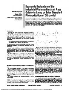
Under an applied tension P, an Euler–Bernoulli beam of mass per unit length and flexural rigidity EI is traveling at a constant speed V between two supports separated by a distance L. A flexible constraint with mass M, stiffness K, and damping constant C is positioned at a location D from the left, upstream end, as shown in Fig. 1. The transverse displacement of the beam, relative to the horizontal X axis, is U(X,T). Without loss of generality, we assume the equilibrium of the beam coincides with the X axis. The friction force between the beam and the constraint is negligible compared to the tension when they are in contact. When the constraint represents a noncontact sensor and actuator, M ⫽0. For a constrained translating string with fixed boundaries at both ends, the stability margin defined by ⌺⫽⫺ sup Re j , where j苸N
j are eigenvalues, vanishes for all constraint locations 关8兴. In what follows, we consider a translating beam with the left end pinned and right end fixed 共other end conditions could have been chosen兲. The necessary and sufficient condition under which ⌺⬎0 will be identified. When V is replaced by ⫺V, the following analysis applies to the translating beam with the upstream end fixed and downstream end pinned. Introduce the following dimensionless parameters: x⫽X/L
u⫽U/L
⫽V 共 L 2 /EI 兲 1/2
d⫽D/L
t⫽T 共 EI/ L 兲
m⫽M / L
4 1/2
2
k⫽KL/EI
(1)
2
u tt 共 x,t 兲 ⫹2 u xt 共 x,t 兲 ⫺ 共 ⫺ 兲 u xx 共 x,t 兲 ⫹u xxxx 共 x,t 兲 ⫽0, 2
0⬍x⬍d,
d⬍x⬍1
u 共 0,t 兲 ⫽u xx 共 0,t 兲 ⫽0 at the pinned end x⫽0
(3a)
u 共 1,t 兲 ⫽u x 共 1,t 兲 ⫽0 at the fixed end x⫽1
(3b)
where the subscripts denote partial differentiations. The conditions across the constraint at x⫽d are u x 共 d ⫹ ,t 兲 ⫽u x 共 d ⫺ ,t 兲
(5a)
共 d ⫹ 兲 ⫽ 共 d ⫺ 兲 , ⬘共 d ⫹ 兲 ⫽ ⬘共 d ⫺ 兲 , ⬙共 d ⫹ 兲 ⫽ ⬙共 d ⫺ 兲 , 共 d ⫹ 兲 ⫺ 共 d ⫺ 兲 ⫽⫺ 共 m 2 ⫹c⫹k 兲 共 d 兲 ,
where and (x) are eigenvalues and eigenfunctions, respectively, and
␥ ⫽ 2⫺ 2
3
(5b)
Critical Speed and Asymptotic Stability
The critical transport speed, i.e., the lowest speed at which divergence instability occurs in the uniform translating beam, is determined first. With the time-derivative terms in Eq. 共2兲 set to zero and the boundary conditions associated with Eqs. 共3a兲 and 共3b兲, nontrivial solutions exist when ␥⬍0 and tan冑⫺ ␥ ⫽ 冑⫺ ␥ . The smallest root for 冑⫺ ␥ , occurring in the interval 冑⫺ ␥ 苸( ,3 /2), is ⫽4.493. Hence by Eq. 共5b兲, the critical speed is 兩 c 兩 ⫽ 冑 2 ⫹  2 ⫽ 冑 2 ⫹4.4932
(6)
Note that the critical speed in the present case lies between those of pinned–pinned 共⫽兲 and fixed–fixed 共⫽2兲 translating beams derived in Wickert and Mote 关13兴. With the constraint at x⫽d, we will show that all the eigenvalues of Eqs. 共5a兲 and 共5b兲 satisfy Re ⭐0 when 兩 兩 ⬍ c . To this end, we first show the following lemma:
J 共 兲 ⫽ 兩兩 ⬙ 共 x 兲 兩兩 2 ⫹ ␥ 兩兩 ⬘ 共 x 兲 兩兩 2 ⫽
冕
1
关 ⬙ 2 共 x 兲 ⫹ ␥ ⬘ 2 共 x 兲兴 dx
(7) is positive definite in the domain ⍀ 1 ⫽ 兵 苸C 关 0,1兴 兩 苸H 4 (0,d)艚H 4 (d,1), (0)⫽ ⬙ (0)⫽ (1)⫽ ⬘ (1)⫽0 其 . 2
Proof: See Appendix A. (2)
with the boundary conditions
u 共 d ⫹ ,t 兲 ⫽u 共 d ⫺ ,t 兲 ,
0⬍x⬍d, d⬍x⬍1,
共 0 兲 ⫽ ⬙ 共 0 兲 ⫽ 共 1 兲 ⫽ ⬘ 共 1 兲 ⫽0,
0
The homogeneous equation describing small transverse motion of the beam is 2
2 共 x 兲 ⫹2 ⬘ 共 x 兲 ⫺ ␥ ⬙ 共 x 兲 ⫹ 共 4 兲 共 x 兲 ⫽0,
Lemma 1. When 兩 兩 ⬍ c , the functional
⫽ PL /EI
c⫽C/ 共 EI L 兲
2 1/2
(4b)
⫺
(4a)
Fig. 1 Schematic of a constrained translating beam with mixed boundary conditions
Journal of Dynamic Systems, Measurement, and Control
We are now in the position to prove the following theorem: Theorem 1. For all subcritical speeds 兩 兩 ⬍ c , all the eigenvalues of Eqs. 共5a兲 and 共5b兲 satisfy Re ⭐0 when c⬎0. Proof: See Appendix B. Based on the assumption that all the eigenvalues of the uniform translating beam are imaginary when 兩 兩 ⬍ c , Theorem 1 can be inferred from Claim 2 of Yang and Mote 关2兴. Setting c⫽0 in Eq. 共B5兲 yields Re ⫽⫽0 when 兩 兩 ⬍ c . Hence the assumption indeed holds in this case. If c⬎0, by Eq. 共B5兲, Re ⫽0 only when (d)⫽0. When (d)⫽0 the eigenvalue problem in Eqs. 共5a兲 and 共5b兲 is identical to that of the uniform translating beam without the constraint. Hence an eigenvalue lies on the imaginary axis only when x⫽d is a nodal point of the corresponding mode of vibration of the uniform translating beam. For a nonvanishing translation speed, however, as noted by Yang 关14兴, eigenfunctions of a uniform translating beam do not have nodal points. This is shown in Section 5 for at least all the high modes. Therefore, when c⬎0, the constrained translating beam is always asymptotically stable, though in cases identified in Section 5, an infinite number of eigenvalues can be arbitrarily close to the imaginary axis. Throughout this work we assume 兩 兩 ⬍ c . JUNE 2000, Vol. 122 Õ 323
4
Characteristic Equation
⌬
The general solution to Eqs. 共5a兲 and 共5b兲 is
共 x 兲⫽
再
A 1 e 1 x ⫹A 2 e 2 x ⫹A 3 e 3 x ⫹A 4 e 4 x , B 1e
1x
⫹B 2 e
2x
⫹B 3 e
3x
⫹B 4 e
4x
0⬍x⬍d
,
(8)
d⬍x⬍1
where A j and B j are arbitrary constants and j are the roots of the fourth-order algebraic equation ( j⫽1,2,3,4):
4 ⫺ ␥ 2 ⫹2 ⫹ 2 ⫽0
(9)
We seek here asymptotic solutions of Eq. 共9兲 for large 兩兩. The fourth-order polynomial in Eq. 共9兲 is factored in the form:
冉
4 ⫺ ␥ 2 ⫹2 ⫹ 2 ⫽ 2 ⫹ 冑2y⫹ ␥ ⫹y⫺
冉
冑2y⫹ ␥
⫻ 2 ⫺ 冑2y⫹ ␥ ⫹y⫹
冊
冑2y⫹ ␥
冊
z ⫹3hz⫹2 f ⫽0
det共 ⌬ 兲 ⫽⌬ 11⌬ 22⫺⌬ 12⌬ 21⫽0
2 f ⫽⫺
2 ␥ ⫹3 2 2 ␥ 3 ⫹ 6 108
Let ⫽ 兩 兩 e . Because Re ⭐0 when 兩 兩 ⬍ c and complex eigenvalues appear in conjugate pairs, we only consider the case with /2⭐⭐. The principal branch of 冑 is given by 冑 ⫽ 冑兩 兩 (cos /2⫹i sin /2), where /4⭐/2⭐/2. Use of the identity 冑2i⫽1⫹i and Eqs. 共15a兲 and 共15b兲 gives
3,4⫽⫺i
(12a)
(14)
册
(15a)
␥ 2 ⫾ ⫹ 共 i 兲 ⫺1/2 ⫾i 冑i⫹O 共 兩 兩 ⫺3/2兲 . 2 4 8
(15b)
The characteristic equation of the eigenvalue problem in Eqs. 共5a兲 and 共5b兲 is derived by applying the associated internal and boundary conditions. By 共0兲⫽⬙共0兲⫽0, we have
再 冎
1 A1 ⫽ 2 A2 1 ⫺ 22
冋
22 ⫺ 23 23 ⫺ 21
22 ⫺ 24 24 ⫺ 21
册再 冎 A3 A4
Next, 共1兲⫽⬘共1兲⫽0 yields
冋
共 2⫺ 3 兲 e 3⫺1 1 B1 ⫽ B2 1⫺ 2 共 3⫺ 1 兲 e 3⫺2
共 2⫺ 4 兲 e 4⫺1 共 4⫺ 1 兲e
4⫺2
(16)
册再 冎
B3 B4 (17)
Application of (d ⫹ )⫽ (d ⫺ ) and ⬘ (d ⫹ )⫽ ⬘ (d ⫺ ), followed by the use of Eqs. 共16兲 and 共17兲, yields two equations relating (B 3 ,B 4 ) T to (A 3 ,A 4 ) T . Use of ⬙ (d ⫹ )⫽ ⬙ (d ⫺ ) and (d ⫹ ) ⫺ (d ⫺ )⫽⫺(m 2 ⫹c⫹k) (d), followed by substitution of Eqs. 共16兲 and 共17兲, and two preceding equations into the resulting expressions, yields a matrix algebraic equation: 324 Õ Vol. 122, JUNE 2000
册
3 ⫺ 4 ⫽ 冑2 兩 兩 ⫺ cos ⫹sin ⫹i cos ⫺sin 2 2 2 2
Substitution of Eq. 共14兲 into Eq. 共10兲 and application of the quadratic formula yields four asymptotic solutions of Eq. 共9兲:
冉 冊 冋 冉 冊
(20)
(22)
Substitution of Eq. 共12b兲 into Eq. 共13兲 and evaluation of the resulting expression yields an asymptotic solution of Eq. 共11兲:
␥ 2 1,2⫽ i⫾ ⫹ 共 i 兲 ⫺1/2⫾ 冑i⫹O 共 兩 兩 ⫺3/2兲 2 4 8
⫹O 共 兩 兩 ⫺1/2兲
2 ⫺ 4 ⫽ i⫺ 冑2 兩 兩 cos ⫹i sin ⫹O 共 兩 兩 ⫺1/2兲 2 2
(13)
␥ 2 y⫽⫺ ⫺ ⫹O 共 兩 兩 ⫺2 兲 2 2
冋
冊册
(11)
By Cardan’s formula for cubic polynomials, one solution to Eq. 共12a兲 is
再 冎
冉
冋
1 ⫺ 2 ⫽ 冑2 兩 兩 cos ⫺sin ⫹i cos ⫹sin 2 2 2 2
(21)
(12b)
z⫽ 共 ⫺ f ⫹ 冑 f 2 ⫹h 3 兲 1/3⫹ 共 ⫺ f ⫺ 冑 f 2 ⫹h 3 兲 1/3
(19)
i
冋冉
冋
⫹O 共 兩 兩 ⫺1/2兲
␥2 , 12
(18)
where entries of matrix ⌬ are given in Appendix C. The characteristic equation of the constrained system is hence obtained from Eq. 共18兲:
where 3h⫽⫺ 2 ⫺
册再 冎
⌬ 12 A 3 ⫽0 ⌬ 22 A 4
(10)
Let z⫽y⫹ ␥ /6, then z satisfies 3
⌬ 11 A3 ⫽ A4 ⌬ 21
3 ⫺ 2 ⫽⫺ i⫺ 冑2 兩 兩 sin ⫺i cos ⫹O 共 兩 兩 ⫺1/2兲 2 2
where y satisfies 2y 3 ⫹ ␥ y 2 ⫺2 2 y⫺ 共 ␥ ⫹ 2 兲 2 ⫽0
再 冎冋
册 冊 冉
冋
冊册 (23)
册
3 ⫺ 1 ⫽⫺ i⫺ 冑2 兩 兩 cos ⫹i sin ⫹O 共 兩 兩 ⫺1/2兲 2 2
(24)
1 ⫺ 4 ⫽ i⫺ 冑2 兩 兩 sin ⫺i cos ⫹O 共 兩 兩 ⫺1/2兲 2 2
(25)
冋
册
Following the reasoning in Chen et al. 关12兴, one can show that for a sufficiently small ␦⬎0, Eq. 共19兲 has no roots of large 兩兩 in the region ⫺␦⬍⭐. Hence we only consider asymptotic solutions of Eq. 共19兲 in /2⭐⭐⫺␦. Because cos /2⬍sin /2 when /4⭐/2⭐/2⫺␦/2, by Eq. 共20兲, 兩 e 1 ⫺ 2 兩 is bounded as 兩兩→⬁. On the other hand, by Eq. 共21兲, 兩 e 3 ⫺ 2 兩 has an exponential rate of decay of at least O(e ⫺ 冑兩 兩 ) for sufficiently large 兩兩. By the same estimations, one can obtain similar terms with exponential rates of decay from Eqs. 共22兲–共25兲. In what follows, we use the same notation O(e ⫺ ␣ 冑兩 兩 ) to denote all the exponentially decaying terms O(e ⫺l 冑兩 兩 ), where l is some positive constant, with ␣⬎0 chosen as the minimum of all such l’s. Hence, for sufficiently large 兩兩, one has e 1 ⫺ 2 ⫽O 共 1 兲
e 3 ⫺ 2 ⫽O 共 e ⫺ ␣ 冑兩 兩 兲
e 3 ⫺ 4 ⫽O 共 e ⫺ ␣ 冑兩 兩 兲
e 2 ⫺ 4 ⫽O 共 e ⫺ ␣ 冑兩 兩 兲
e 3 ⫺ 1 ⫽O 共 e ⫺ ␣ 冑兩 兩 兲
e 1 ⫺ 4 ⫽O 共 e ⫺ ␣ 冑兩 兩 兲
(26)
We multiply Eq. 共19兲 by ( 1 ⫺ 2 )e 1 ⫺ 4 , estimate the order of magnitude of each term by use of Eq. 共26兲, and include all the resulting terms with exponential rates of decay into O(e ⫺ ␣ 冑兩 兩 ). Through a careful and lengthy evaluation, one obtains the following asymptotic expression for the characteristic equation: C 1 e 1 ⫺ 2 ⫹C 2 e 共 1 ⫺ 2 兲 d ⫹C 3 e 共 1 ⫺ 2 兲共 1⫺d 兲 ⫹C 4 ⫽O 共 e ⫺ ␣ 冑兩 兩 兲 (27) where ␣ is a positive constant and C 1 ⫽ 共 1 ⫺ 4 兲共 22 ⫺ 23 兲 ⫹ 共 m 2 ⫹c⫹k 兲共 22 ⫺ 23 兲
冋
⫻
1 1 ⫺ 共 2 ⫺ 4 兲共 3 ⫺ 4 兲 共 1 ⫺ 2 兲共 1 ⫺ 3 兲
册
(28a)
Transactions of the ASME
C 2 ⫽ 共 m 2 ⫹c⫹k 兲
2⫹ 3 1⫺ 2
(28b)
C 3 ⫽ 共 m 2 ⫹c⫹k 兲
1⫹ 3 1⫺ 2
(28c)
essary to include them in Eq. 共32兲 for subsequent analysis. Substitution of Eq. 共32兲 into Eq. 共31兲 yields after simplification e 2 冑i ⫽i⫺
C 4 ⫽ 共 2 ⫺ 4 兲共 23 ⫺ 21 兲 ⫹ 共 m 2 ⫹c⫹k 兲共 23 ⫺ 21 兲
冋
1 1 ⫻ ⫹ 共 1 ⫺ 4 兲共 3 ⫺ 4 兲 共 1 ⫺ 2 兲共 2 ⫺ 3 兲
册
⫺ (28d)
Substitution of Eqs. 共15a兲 and 共15b兲 into Eqs. 共28a兲–共28d兲 gives the coefficients C j ( j⫽1,2,3,4) in the following asymptotic forms: C 1 ⫽2 共 1⫹i 兲 i 冑i⫹ 共 m ⫹c⫹k 兲关 ⫺1⫹O 共 兩 兩 2
C 2 ⫽⫺ C 3⫽
冋
冋
册
⫺1
兲兴 ⫹O 共 冑兩 兩 兲 (29a)
1⫺i ⫹O 共 兩 兩 ⫺1 兲 共 m 2 ⫹c⫹k 兲 ⫹O 共 1 兲 2
册
1⫹i ⫹O 共 兩 兩 ⫺1 兲 共 m 2 ⫹c⫹k 兲 ⫹O 共 1 兲 2
(29c)
Note that within the order of approximation, the coefficients C j ( j⫽1,2,3,4) are independent of ␥ and in Eqs. 共29a兲–共29d兲. The dependence of the characteristic equation on these parameters remains in the exponents in Eq. 共27兲.
2 共 x 兲 ⫹2 ⬘ 共 x 兲 ⫺ ␥ ⬙ 共 x 兲 ⫹ 共 4 兲 共 x 兲 ⫽0,
0⬍x⬍1 (30a)
共 0 兲 ⫽ ⬙ 共 0 兲 ⫽ 共 1 兲 ⫽ ⬘ 共 1 兲 ⫽0
(30b)
all the eigenfunctions (x) of higher modes do not have nodal points when 0⬍ 兩 兩 ⬍ c . Proof: See Appendix D. The proof for a more general case when one considers also lower modes remains unavailable and is a subject of future investigation. Next, the asymptotic behavior of eigenvalues of large modulus is analyzed by using the asymptotic expression of the characteristic equation given by Eqs. 共27兲 and 共29a兲–共29d兲. 5.1 Asymptotic Behavior of Eigenvalues for mÄ0. Substituting Eqs. 共29a兲–共29d兲 into Eq. 共27兲, including all the terms in the order symbols in their leading order term, and dividing the resulting expression by 2 关 2(i⫺1) 冑i⫺c 兴 , yields 4 冑i
⫽i⫹
e 共 1⫺2 兲d⫺
c 2 冑i
By Eq. 共15a兲 we have
冊冑
i i
ci 4 冑i
冉
冊
␥ 2 1 ⫺ 2 ⫽2 冑i⫹ ⫹ 共 i 兲 ⫺1/2⫹O 共 兩 兩 ⫺1 兲 2 4
(33)
(34)
冏
e 冑2 兩 兩 共 cos /2⫺sin /2兲 ⫽ i⫺ ⫺
冉
c
e ⫺ 共 /2兲 i 关 P 1 ⫹ P 2 ⫹ 共 P 2 ⫺ P 1 兲 i 兴
4 冑2 兩 兩
␥ 2 ⫹ 2 4
冊 冑冑 冏 i
⫹O 共 兩 兩 ⫺1 兲
(35)
Because 兩 e 2d 冑i 兩 ⫽ 兩 e d 冑2 兩 兩 ( cos /2⫺sin /2) 兩 and cos /2⬍sin /2 when /4⭐/2⬍/2, e 2d 冑i is bounded. Similarly, e 2 ( 1⫺d ) 冑i is bounded. Hence by Eq. 共34兲, P 1 ⫹i P 2 is bounded for large 兩兩. By Eq. 共35兲, one has e 冑2 兩 兩 共 cos /2⫺sin /2兲 ⫽1⫹O 共 兩 兩 ⫺1/2兲
(36)
By Eq. 共36兲, 冑2 兩 兩 (cos /2⫺sin /2)→0 as 兩兩→⬁. Hence all eigenvalues of large modulus satisfy as 兩 兩 →⬁
(37)
The logarithms of both sides of Eq. 共35兲, followed by the use of Taylor expansion, yields
冑兩 兩
冉
冊 再冋
cos ⫺sin 2 2
⫽⫺ ⫺
1
冑兩 兩
冉
c 共 P 2 ⫺ P 1 兲 cos ⫺ 共 P 2 ⫹ P 1 兲 sin 8 2 2
1 ␥ 2 ⫹ 2 2 4
冊冉
cos ⫺sin 2 2
冊冎
⫹O 共 兩 兩 ⫺1 兲
册 (38)
Dividing Eq. 共33兲 by the imaginary part of its left-hand side and using Eq. 共35兲 yields e ⫺i 冑2 兩 兩 共 cos /2⫹sin /2兲 ⫽⫺i⫹O 共 兩 兩 ⫺1/2兲
(39)
The logarithms of both sides of Eq. 共39兲 and a Taylor expansion yields
冉
冊
s⫽ 冑2 兩 兩 cos ⫹sin ⫽2 j ⫹ ⫹O 共 j ⫺1 兲 2 2 2
(40)
where j苸N. Hence by Eqs. 共40兲 and 共37兲, 兩 j 兩 ⫽( j ) 2 关 1 ⫹O( j ⫺1 ) 兴 . Multiplying both sides of Eq. 共38兲 by 冑兩 兩 and using Eq. 共37兲 yields
e 共 1 ⫺ 2 兲共 1⫺d 兲
⫹O 共 兩 兩 ⫺1 兲
⫹O 共 兩 兩 ⫺1 兲
Equation of the moduli of both sides of Eq. 共33兲 yields
→ /2
Theorem 2. For the eigenvalue problem of the uniform translating beam:
c
␥ 2 ⫹ 2 4
e ⫺ /2关 P 1 ⫹ P 2 ⫹ 共 P 2 ⫺ P 1 兲 i 兴
P 1 ⫹i P 2 ⫽e 2d 冑i ⫺ie 2 共 1⫺d 兲 冑i ⫺2
Spectral Analysis
As mentioned earlier, unlike the case of a translating string, eigenfunctions of a translating beam do not have nodal points. Here we provide a theoretical proof for at least all the high modes.
e 1⫺2⫹
4 冑2 兩 兩
where P 1 , P 2 苸R satisfy
(29b)
C 4 ⫽2 共 1⫺i 兲 i 冑i⫹ 共 m 2 ⫹c⫹k 兲关 1⫹O 共 兩 兩 ⫺1 兲兴 ⫹O 共 冑兩 兩 兲 (29d)
5
冉
c
(31)
冉
兩 兩 cos
冊
c ⫺sin → P 1 cos 2 2 4 4
Hence by Eqs. 共41兲 and 共37兲, one obtains (32)
Note that though the high-order terms in Eqs. 共15a兲 and 共15b兲 that involve ␥ and were not used in previous derivations, it is necJournal of Dynamic Systems, Measurement, and Control
冉
Re ⫽ 兩 兩 cos ⫽ 兩 兩 cos
⫺sin 2 2
as 兩 兩 →⬁
冊冉
as 兩 兩 →⬁
(41)
冊
c cos ⫹sin → P 1 2 2 4 (42)
JUNE 2000, Vol. 122 Õ 325
It is interesting to note that, because of Eq. 共37兲, the asymptotic behavior of Re becomes independent of ␥ and in Eq. 共42兲. By Eqs. 共34兲 and 共40兲, we have P 1 ⫽e d 冑2 兩 兩 共 cos /2⫺sin /2兲 cos ds⫹e 共 1⫺d 兲 冑2 兩 兩 共 cos /2⫺sin /2兲 ⫻sin共 1⫺d 兲 s
(43)
By Eqs. 共43兲 and 共37兲, P 1 →2 cos ds ⫺2 as 兩兩→⬁. Hence we obtain the desired asymptotic expression for the real parts of eigenvalues of large modulus: Re →⫺
c 关 1⫺cos ds 兴 2
as 兩 兩 →⬁
(44)
It is seen that asymptotic rates of decay of all modes of vibration are proportional to the damping constant c. The dependence of eigenvalues on the location of the constraint is discussed next. Rational d. Let d⫽p/q, where p,q苸N and (p,q)⫽1. By Eq. 共40兲, cos ds⫽cos关2np/q⫹p/2q⫹O(n ⫺1 ) 兴 . Hence by Eq. 共44兲, all the eigenvalues are asymptotic to at most q lines of constant ⫽Re ⭐0. The necessary and sufficient condition for one of these asymptotic lines to coincide with the imaginary axis, i.e., ⫽0, is given by the following theorem:
sufficiently high modes, leading to a qualitatively different behavior of the distributed model. While the stability margin for any finite number of modes varies continuously with d, it is characterized by abrupt changes when the number of included modes increases. In real applications, favorable control locations, resulting in relatively large stability margins of the distributed model, correspond to rational numbers that are not expressible in the form 4p/(4q⫺1) and have small denominators and numerators. In general, increasing the denominator and numerator of d reduces the stability margin of the distributed model. This is expected as when the denominator and numerator increase, d approaches an irrational number. 5.2 Asymptotic Behavior of Eigenvalues for mÅ0. When m⫽0, all the eigenvalues of large modulus approach the imaginary axis, similar to the case of the constrained translating string in Zhu et al. 关8兴. Because of the same asymptotic behavior of eigenvalues for all d, we consider only the case when d⫽1/2. Substitution of Eqs. 共29a兲–共29d兲 into Eq. 共27兲, combination of all the terms in the order symbols in their leading order term, application of the quadratic formula, and substitution of Eq. 共32兲 into the resulting expression, yields e 冑i ⫽
Theorem 3. When m⫽0, c⫽0, and d is rational, a branch of eigenvalues of Eqs. 共5a兲 and 共5b兲 of large modulus approaches the imaginary axis if and only if d⫽4p/(4q⫺1), where p,q苸N. Proof: See Appendix E. Because eigenvalues of the lower modes are finite in number, by Theorem 3, the system of Eqs. 共5a兲 and 共5b兲 has a positive, uniform stability margin ⌺ if and only if d assumes rational values not of the form 4p/(4q⫺1), where p,q苸N. Under such constraint locations, when c⬎0, all the modes of vibration are dissipated at a minimal rate ⌺ under arbitrary disturbances. The center location d⫽1/2, for instance, is not expressible in the form 4p/(4q⫺1). Hence there exists ⌺⬎0 such that Re j ⬍⫺⌺ for all j苸N. By Eq. 共40兲, cos ds⫽cos关 j⫹/4⫹O( j ⫺1 ) 兴 . When j is even, cos ds→冑2/2 as j→⬁. When j is odd, cos ds →⫺冑2/2 as j→⬁. Hence, Re →⫺c关2⫾冑2 兴 /4 as 兩兩→⬁. All the eigenvalues of high modes are distributed along two straight lines in the left-half plane parallel to the imaginary axis. Similar results are obtained in Chen et al. 关12兴 for the special case with P⫽ ⫽0. Irrational d. When d is irrational, there always exists a branch of eigenvalues approaching the imaginary axis. The following lemma by Hardy and Wright 关15兴 is used in the proof of Theorem 4. Lemma 2. For any irrational d, given arbitrary b, and positive R and , there exist integers n and S, such that n⬎R and 兩 nd⫺S ⫺b 兩 ⬍.
326 Õ Vol. 122, JUNE 2000
共 i 兲 ⫺1/2
(45)
Equating the moduli of both sides of Eq. 共45兲 gives e 冑兩 兩 /2共 cos /2⫺sin /2兲 ⫽1⫹
冑2 2
冉
冋冉
冊 冉 冊册
2 ␥ 2 1 ⫺1⫾ ⫺ ⫹ m 4 8 冑3
冊
⫻ cos ⫺sin 兩 兩 ⫺1/2⫹O 共 兩 兩 ⫺1 兲 2 2 (46) The logarithms of both sides of Eq. 共46兲 and use of the Taylor expansion yields
冊冋 冉 冉
冉
冊 冉 冊册
2 ␥ 2 1 兩 兩 1/2 cos ⫺sin ⫽ ⫺1⫾ ⫺ ⫹ 2 2 m 4 8 冑3
冊
⫻ cos ⫺sin 兩 兩 ⫺1/2⫹O 共 兩 兩 ⫺1 兲 2 2 (47)
From Eq. 共47兲 one obtains cos /2⫺sin /2⫽O( 兩 兩 ⫺1 ). Hence →/2 as 兩兩→⬁. By Eq. 共47兲 one has Re ⫽ 兩 兩 cos ⫽
冉
冋冉
冊 冉 冊册冉
1 2 ␥ 2 ⫺1⫾ ⫺ ⫹ m 4 8 冑3
冊
cos ⫺sin 2 2
⫻ cos ⫹sin ⫹O 共 兩 兩 ⫺1/2兲 ⫽O 共 兩 兩 ⫺1/2兲 2 2
Proof: See Appendix F.
Remark. Rational locations that are not of the form 4p/(4q ⫺1) result in a positive stability margin for the distributed model in Eqs. 共5a兲 and 共5b兲, while all others possess a zero stability margin. Because the types of locations can be arbitrarily close, the stability margin of the distributed model is infinitely sensitive to d. This occurs because the sensitivity of each eigenvalue to d increases with the mode number. An infinitesimal change in d can result in a significant variation in distribution of eigenvalues of
冊 冉 冊册
⫹O 共 兩 兩 ⫺1 兲
Theorem 4. When m⫽0, c⫽0, and d is any irrational number, there always exists a family of eigenvalues of Eqs. 共5a兲 and 共5b兲 of large modulus which approaches the imaginary axis. Though all the eigenvalues remain strictly in the left-half plane, an infinite number of them are arbitrarily close to the imaginary axis for irrational d. Hence ⌺⫽0 and the system is not exponentially stable.
再 冋冉 冎
2 ␥ 2 i⫾ 冑3 1 1⫹ ⫺1⫾ ⫺ ⫹ 2 m 4 8 冑3
冊
(48)
Hence all the eigenvalues of high modes approach the imaginary axis in the order O( 兩 兩 ⫺1/2). Though any tiny inertia m can render the distributed model nonexponentially stable, it will not dramatically alter the stability margin for the finite number of modes within the bandwidth for control in practical applications. The use of a noncontact sensor and actuator can eliminate the inertia effect of a collocated control device.
6
Numerical Solution
Eigenvalues for any finite number of modes can be calculated numerically. To this end, spatial discretization of Eqs. 共2兲–共4c兲 by Galerkin’s method is used. The solution is represented by an expansion series Transactions of the ASME
N
u 共 x,t 兲 ⫽
兺 共 t 兲⌰ 共 x 兲 j⫽1
j
(49)
j
where ⌰ j are trial functions, j are generalized coordinates, and N is the number of included modes. In the examples shown in Section 7, we choose ⌰ j (x) as eigenfunctions of a stationary, Euler–Bernoulli beam with pinned-fixed boundaries: ⌰ j 共 x 兲 ⫽cosh a j 共 1⫺x 兲 ⫺cos a j 共 1⫺x 兲 ⫺b j 关 sinh a j 共 1⫺x 兲 ⫺sin a j 共 1⫺x 兲兴
(50)
where a j are the roots of the frequency equation tan a j⫽tanh a j and b j ⫽(cosh a j⫺cos a j)/(sinh a j⫺sin a j) 关16兴. The eigenfunctions in Eq. 共50兲 satisfy the boundary conditions in Eqs. 共3a兲 and 共3b兲, and they are orthogonal, that is, 兰 10 ⌰ i (x)⌰ j (x)dx⫽0 if i ⫽ j. The discretized model for Eqs. 共2兲–共4b兲 is N
兺 关m j⫽1
¨ j 共 t 兲 ⫹ 共 g i j ⫹c i j 兲 ˙ j 共 t 兲 ⫹k i j j 共 t 兲兴 ⫽0, i j
i⫽1,2, . . . ,N (51)
where
冕 冕
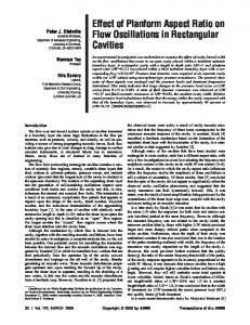
Fig. 2 Distribution of the first 20 eigenvalues for m Ä0, c Ä1, d Ä1Õ2, and N Ä20. Other parameters are: „a… Ä0.1, Ä5, and k Ä2 „‘‘Ã’’…; „b… Ä0.5, Ä1, and k Ä0 „‘‘¿’’….
1
mi j⫽
⌰ i 共 x 兲 ⌰ j 共 x 兲 dx⫹m⌰ i 共 d 兲 ⌰ j 共 d 兲
(52a)
0
g i j ⫽2
1
⌰ i 共 x 兲 ⌰ ⬘j 共 x 兲 dx,
0
k i j⫽共 2⫺ 2 兲 ⫻
冕
冕
1
c i j ⫽c⌰ i 共 d 兲 ⌰ j 共 d 兲
(52b)
⌰ i⬘ 共 x 兲 ⌰ ⬘j 共 x 兲 dx⫹a i4
0
1
⌰ i 共 x 兲 ⌰ j 共 x 兲 dx⫹k⌰ i 共 d 兲 ⌰ j 共 d 兲
(52c)
0
The mass m i j , stiffness k i j , and damping c i j matrices are symmetric, while the gyroscopic matrix g i j is skew-symmetric. By defining y⫽ 关 ˙ T , T 兴 T , where ⫽ 关 1 , 2 , . . . , N 兴 T , we transform Eq. 共51兲 into an equivalent set of 2N first order ordinary differential equations. The eigenvalues of the resulting first-order system, j ⫽ j ⫾i j ( j⫽1,2, . . . ,N), where j , j 苸R, are subsequently determined through numerical solution of a generalized eigenvalue problem.
7
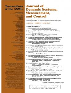
Fig. 3 Distribution of the first 20 eigenvalues for m Ä0, c Ä1, d Ä4Õ5, and N Ä20. Other parameters are: „a… Ä0.1, Ä5, and k Ä2 „‘‘Ã’’…; „b… Ä0.5, Ä1, and k Ä0 „‘‘¿’’….
Results and Discussion
7.1 Distribution of Eigenvalues. Eigenvalues for different cases are calculated numerically and compared with the analytical predictions given in Section 5. The first 20 eigenvalues for d ⫽1/2, ⫽0.1, ⫽5, m⫽0, c⫽1, k⫽2, and N⫽20 are shown in Fig. 2. All the eigenvalues are asymptotic to the two lines, Re ⫽⫺0.146 and Re ⫽⫺0.85, in the left-half plane, as predicted in Section 5.1. The second mode has a minimal decay rate 兩 2 兩 ⫽0.121, hence the stability margin of the distributed model is ⌺⫽0.121. When ⫽0.5, ⫽1, and k⫽0 with other parameters unchanged, the asymptotic behavior of eigenvalues remains unaltered, as expected, but the first several eigenvalues of lower modes are shifted. As a result, the stability margin of the distributed model increases to ⌺⫽0.146. When the tension is increased, the beam model becomes more string-like and the constraint location approaches the node of the second mode of vibration for the translating string model. The decay rate of the second mode of vibration, and consequently, the distributed model is reduced. When d⫽4/5 with other parameters same as those in Fig. 2, the first 20 eigenvalues are shown in Fig. 3. As predicted by Eq. 共44兲, there are five families of eigenvalues: one of them approaches the imaginary axis because d can be expressed as 4p/(4q⫺1) with p⫽3 and q⫽4, two are asymptotic to Re ⫽⫺0.345, and two to Re ⫽⫺0.904. When ⫽0.5, ⫽1, and k⫽0 with other parameters unchanged, though the first several eigenvalues of lower Journal of Dynamic Systems, Measurement, and Control
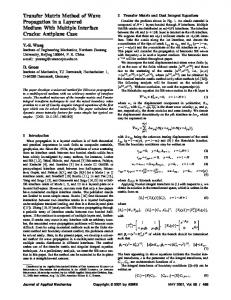
modes are altered, the asymptotic behavior of eigenvalues remains unchanged. The stability margin is 4.79⫻10⫺6 when N⫽20 and vanishes as N→⬁. When m⫽0 with other parameters same as those in Fig. 2共a兲, all the eigenvalues of higher modes approach the imaginary axis 共not shown兲, as predicted in Section 5.2. When m is increased from 0 to 0.2, the stability margin of the first 20 modes decreases monotonically from 0.121 to 2.55⫻10⫺3 . 7.2 Sensitivity of the Stability Margin to Variation of d. For the case of Fig. 2共a兲, the sensitivity of the stability margin of the first N modes to variation of d in the vicinity of the center location is shown in Fig. 4. The stability margin varies more dramatically with d when N is increased. As noted earlier, d⫽1/2 is a favorable location with a resulting stability margin of 0.121 for the distributed model. The stability margin at the center location is independent of N as long as N⭓2, because the second eigenvalue has the shortest distance to the imaginary axis. Within the range of d shown in the figure, a maximal stability margin of 0.246 is predicted at d⫽0.52275 by a ten-mode analysis. The stability margin at this location drops to 0.0028 when N⫽17. Common practice predicts the optimal locations from spatially discretized models. However, the stability margin at such a location often drops sharply when higher modes are accounted for. JUNE 2000, Vol. 122 Õ 327
location. For d⫽2/3, the stability margin of the distributed model is the same 共i.e., 0.236兲 as that of the first 20 modes, because the third modes has the shortest distance to the imaginary axis. The stability margins at the constraint locations not included as nodes cannot be larger than that at d⫽2/3 because of their relatively large numerators and/or denominators. Hence, d⫽2/3 is the optimal location associated with the maximal stability margin of the distributed model. The center location corresponds to the second largest stability margin of the distributed model. The range of variation of d around the optimal location to ensure a minimal stability margin of 0.236 for the first 20 modes is smaller than that around the center location shown in Fig. 4共c兲. The optimal location identified can be used for the placement of a control device. It offers an opportunity to stabilize a largest number of modes without increasing the bandwidth of any control hardware. Fig. 4 Variation of the stability margin of the first N modes with the constraint location around the center location: „a… N Ä2, „b… N Ä10, „c… N Ä20, „d… N Ä40, and „e… N Ä80. Other parameters are the same as those in Fig. 2„a…. The interval d «†0.495,0.53‡ is divided into a mesh of 141 nodes.
When d is increased from 1/2, it is seen that the stability margin increases first and drops subsequently. Due to the nonsymmetric boundary conditions, the stability margin drops rapidly when the constraint is placed slightly to the left of the center location. For all N⬎2, there exist regions in the neighborhood of the center location, in which the stability margins coincide with that for N ⫽2. These regions of coincidence decrease with the increase of N and reduce to a single point 共1/2,0.121兲 when N→⬁. In the vicinity of the center location, the ranges of variation of d to ensure a minimal stability margin of 0.121 for the first N modes are 关0.5,0.5136兴 for N⫽20, 关0.5,0.50667兴 for N⫽40, and 关0.5,0.5033兴 for N⫽80. When the control device is located within these ranges, the stability margins at the center location can be guaranteed for the specified numbers of modes. The qualitatively differing behaviors of the distributed model in Eqs. 共5a兲 and 共5b兲 for small variations in d can be interpreted as follows. For a rational d of the form 4p/(4q⫺1) or an irrational d near the center location, though the stability margin of the first N modes can be larger than that for the center location, they vanish when N→⬁. On the other hand, for a rational d near the center location that is not expressible in the form 4p/(4q⫺1), the stability margin of the distributed model does not vanish, but it remains small because of the relatively large denominator and numerator of d. 7.3 Optimal Constraint Location. The asymptotic behavior of eigenvalues predicted in Section 5.1 is used to predict the constraint location associated with the maximal stability margin of the distributed model. Standard optimization techniques cannot be applied here because of the infinite sensitivity of the stability margin to d. Consider the case of Fig. 2共a兲 with the interval 0⬍d⬍1 divided into a sufficiently fine mesh that includes favorable locations identified in Section 5.1 as nodes. The stability margin of the first 20 modes at each node is calculated first numerically 共not shown here兲. Due to the relatively large number of modes included, sharp peaks are observed around the set of favorable locations, such as 2/3, 1/2, 2/5, 1/3, in order of decreasing peak amplitudes. Though the stability margin in a small neighborhood to the right of each of these locations, say, d⫽1/2, can be slightly larger than that at d⫽1/2, as shown in Section 7.2, it is reduced substantially when higher modes are included. However, the stability margins at the favorable locations remain unchanged when higher modes are included. Because the stability margin at any d either decreases or remains unchanged when the number of included modes is increased, the stability margin of the distributed model at any location cannot be greater than that of the first 20 modes at the same 328 Õ Vol. 122, JUNE 2000
8
Conclusions
1 At all subcritical speeds, the constrained translating beam is asymptotically stable when c⬎0. When m⫽0, c⬎0, and d is either a rational number of the form 4p/(4q⫺1), where p, q 苸N, or an irrational number, a branch of eigenvalues approaches the imaginary axis. All the other eigenvalues are either asymptotic to at most q⫺1 lines of constant Re in the left-half plane when d is rational, or scattered all over in the left half plane when d is irrational. When m⫽0, all the eigenvalues of high modes approach the imaginary axis in the left-half plane independent of other parameters. In all these cases, stability margins of the distributed translating beam vanish, and the system is not exponentially stable. 2 When m⫽0, c⬎0, and d is any rational not expressible in the form 4p/(4q⫺1), where p,q苸N, all the eigenvalues are asymptotic to at most q lines of constant Re in the left-half plane. The system has a guaranteed stability margin for all the modes of vibration. 3 The asymptotic distribution of eigenvalues is governed by the location, inertia, and damping constant of the constraint. Though the tension, transport speed, and constraint stiffness do not influence the asymptotic behavior of eigenvalues of high modes, by affecting eigenvalues of low modes, they can alter the stability margin of the distributed system. 4 The optimal location d⫽2/3 corresponds to the maximal stability margin of the distributed model analyzed here. When it is desirable to dissipate a largest number of modes possible, the control device can be placed in a sufficiently small neighborhood of a favorable location such as 2/3 or 1/2, the allowable range around which depends on the number of modes to be controlled, the stability margin of the finite number of modes within a desired bandwidth has at least the same amplitude as that at the favorable location. Stabilization of a largest number of modes can be achieved in this case without increasing the bandwidth of any control device. 5 The methodology developed in this work can be extended to predict eigenvalues and stability margins of controlled translating beams with different boundary conditions and controller designs. It can also be used to determine the optimal control parameters resulting in maximal stability margins of distributed systems.
Acknowledgments This work was supported by an Earmarked Grant of the Hong Kong Research Grants Council and a Postdoctoral Fellowship of the Chinese University Hong Kong.
Nomenclature A, A j , B j ( j⫽1,2,3,4) a j ( j⫽1,2, . . . ) b; b j ( j⫽1,2, . . . ) C,c; c i j (i, j⫽1,2, . . . ,N)
⫽ ⫽ ⫽ ⫽
integration constants roots of frequency equation arbitrary constant; coefficients damping constant; entries of damping matrix Transactions of the ASME
C j ( j⫽1,2,3,4) D,d EI F j ( j⫽1,2,3,4), f g i j (i, j⫽1,2, . . . ,N) h i
⫽ ⫽ ⫽ ⫽ ⫽ ⫽ ⫽
J( ),Jˆ ( ); j, j ⬘ ⫽ K,k; k i j ⫽ k j ( j⫽1,2,3,4) ⫽ L;l; l 1 , l 2 ⫽ M ,m; m i j (i, j⫽1,2, . . . ,N) ⫽ N; n,n ⬘ , n j , N j ( j⫽1,2, . . . ) ⫽ P; P 1 , P 2 ⫽ p,p ⬘ , q,q ⬘ ⫽ R;r ⫽ S; s,s j ( j⫽1,2, . . . ) T,t U(X,T),u(x,t) V, ; c w X,x y,z; y
⫽ ⫽ ⫽ ⫽ ⫽ ⫽ ⫽
␣ ⫽  ⫽ ⌬,⌬ i j ⫽
␦ , ⑀ , ⑀ j ( j⫽1,2, . . . ) ␥ j (t)( j⫽1,2, . . . )
⫽ ⫽ ⫽ ⫽
⫽ , j ( j⫽1,2,3,4) ⫽
;⌺ ⫽ ⍀ j ( j⫽1,2,3); ⫽
(x), 1 , 2 ⫽ (x) ⌰ j ( j⫽1,2, . . . ); 1 , 2
⫽ ⫽ ⫽ ⫽ ⫽
coefficients constraint location bending stiffness coefficients entries of gyroscopic matrix coefficient imaginary unit or integer index functionals; integers constraint stiffness; entries of stiffness matrix integers span length; positive constant; integers constraint mass; entries of mass matrix number of included modes; integers tension; real and imaginary parts of a complex variable integers positive constant; location of assumed node integer; real variables time displacement transport speed; critical speed integer spatial variable variables of polynomials of order three; state variable positive constant smallest root for 冑⫺ ␥ coefficient matrix and its entries positive constants effective tension generalized coordinates square root of dimensionless tension eigenvalue variable and roots of characteristic polynomial real part of eigenvalue; stability margin function spaces; imaginary part of eigenvalue eigenfunction and its real and imaginary parts derivative of eigenfunction mass density trial functions; phase angle Lagrangian multipler coefficients
J 共 兲 ⫽Jˆ 共 兲 ⫽ 兩兩 ⬘ 共 x 兲 兩兩 2 ⫹ ␥ 兩兩 共 x 兲 兩兩 2 ⫽
冕
1
关 ⬘ 2 共 x 兲 ⫹ ␥ 2 共 x 兲兴 dx
0
(A1) Therefore, inf J( )⭓ min Jˆ ( ). 苸⍀ 2
苸⍀ 3
We now show that when ␥ ⬎⫺  2 , min Jˆ()⫽0. If ␥⭓0, it is 苸⍀3
obvious that min Jˆ()⫽0. For ⫺  2 ⬍ ␥ ⬍0, the minimum of Jˆ ( ) 苸⍀3
subject to the constraint 兰 10 (x)dx⫽0 is obtained by method of calculus of variation. The corresponding Euler’s equation along with the constraint and boundary conditions are derived by applying the Theorems I.2 and III.2 in Wan 关17兴:
⬙ 共 x 兲 ⫽ ␥ 共 x 兲 ⫹ ⬘ 共 0 兲 ⫽0,
共 1 兲 ⫽0,
冕
1
(A2)
共 x 兲 dx⫽0
(A3)
0
where is the Lagrangian multiplier. Solution to Eq. 共A2兲 by use of the first equation in Eq. 共A3兲 yields
共 x 兲 ⫽A cos冑⫺ ␥ x⫺
␥
(A4)
where A is a constant. Applying the second and third equations in Eq. 共A3兲 to Eq. 共A4兲 gives A cos冑⫺ ␥ ⫺
⫽0, ␥
A
冑⫺ ␥
sin冑⫺ ␥ ⫺
⫽0 ␥
(A5)
Hence A tan冑⫺ ␥ ⫽A 冑⫺ ␥ by Eq. 共A5兲. Because tan冑⫺ ␥ ⫽ 冑⫺ ␥ has no solutions in 0⬍ 冑⫺ ␥ ⬍  , one has A⫽0. Consequently, ⫽0 by Eq. 共A5兲. Therefore the only solution to Eqs. 共A2兲 and 共A3兲 is ⬅0. Hence, min Jˆ()⫽Jˆ(0)⫽0. 苸⍀3
Because ␥ ⬎⫺  2 implies 兩 兩 ⬍ c , one concludes that J( ) ⭓0 for all 苸⍀ 1 when 兩 兩 ⬍ c . Furthermore, it can be easily shown that J( )⫽0 if and only if ⫽0. Hence, Lemma 1 holds.
Appendix B
Proof of Theorem 1
¯ (x), Multiplying both sides of the first equation in Eq. 共5a兲 by where the overbar denotes complex conjugation, integrating the resulting expression in 关0,1兴 by parts by use of the boundary and internal conditions in Eq. 共5a兲, and noting that 2
冕
1
0
¯ dx⫽2 ⬘
冕
1
关 1⬘ 1 ⫹ 2⬘ 2 ⫹i 共 1 2⬘ ⫺ 2 1⬘ 兲兴 dx
0
⫽ 关 21 共 1 兲 ⫺ 21 共 0 兲 ⫹ 22 共 1 兲 ⫺ 22 共 0 兲兴 ⫹4 i
冕
1
0
1 2⬘ dx⫽4 i 具 1 , 2⬘ 典
(B1)
where ⫽ 1 ⫹i 2 and 1 and 2 are real, one obtains 2 兩兩 兩兩 2 ⫹4 i 具 1 , 2⬘ 典 ⫹ ␥ 兩兩 ⬘ 兩兩 2 ⫹ 兩兩 ⬙ 兩兩 2
Appendix A
Proof of Lemma 1
⫹ 共 m 2 ⫹c⫹k 兲 兩 共 d 兲 兩 2 ⫽0
(B2)
The functions contained in ⍀ 1 are twice continuously differentiable and satisfy the boundary conditions in Eq. 共5a兲. Their distributional derivatives up to the fourth order are square integrable in (0,d) and (d,1). Define a new domain ⍀ 2 ⫽ 兵 苸C 3 关 0,1兴 兩 (0)⫽ (1)⫽ ⬘ (1)⫽0 其 . Because ⍀ 2 is dense in ⍀ 1 共for each element in ⍀ 1 there exists an arbitrarily close element in ⍀ 2 兲, inf J( )⫽ inf J( ). Let ⫽⬘ and ⍀ 3 ⫽ 兵
Let ⫽ ⫹i , where , 苸R. Separating the real and imaginary parts in Eq. 共B2兲 yields
For every in ⍀ 2 , there cor-
Multiplying Eq. 共B3兲 by and Eq. 共B4兲 by , and adding the two expressions, yields
苸⍀ 1
苸⍀ 2 苸C 2 关 0,1兴 兩 (1)⫽ 兰 10 (x)dx⫽0 其 .
responds an element in ⍀ 3 with
Journal of Dynamic Systems, Measurement, and Control
共 2 ⫺ 2 兲 兩兩 兩兩 2 ⫹ ␥ 兩兩 ⬘ 兩兩 2 ⫹ 兩兩 ⬙ 兩兩 2
⫹ 关 m 共 2 ⫺ 2 兲 ⫹c ⫹k 兴 兩 共 d 兲 兩 2 ⫽4 具 1 , ⬘2 典
(B3)
2 兩兩 兩兩 2 ⫹4 具 1 , 2⬘ 典 ⫹ 关 2 m⫹c 兴 兩 共 d 兲 兩 2 ⫽0 (B4)
JUNE 2000, Vol. 122 Õ 329
兵 共 2 ⫹ 2 兲 兩兩 兩兩 2 ⫹ ␥ 兩兩 ⬘ 兩兩 2 ⫹ 兩兩 ⬙ 兩兩 2 ⫹ 关 m 共 ⫹ 兲 ⫹k 兴 兩 共 d 兲 兩 其 ⫽⫺c 共 ⫹ 兲 兩 共 d 兲 兩 2
2
2
2
2
2
再 冎
1 A1 ⫽ 2 ⫹r 1 1 ⫹r 2 A2 e ⫺e
(B5)
⫻
By Lemma 1, ␥ 兩兩 ⬘ 兩兩 2 ⫹ 兩兩 ⬙ 兩兩 2 ⭓0 when 兩 兩 ⬍ c . Hence by Eq. 共B5兲, Re ⫽⭐0 when c⬎0.
冋
e 3 ⫹r 2 ⫺e 2 ⫹r 3 e
1 ⫹r 3
⫺e
e 4 ⫹r 2 ⫺e 2 ⫹r 4
3 ⫹r 1
e
1 ⫹r 4
⫺e
4 ⫹r 1
册再 冎 A3 A4
(D2) Combining Eqs. 共19兲 and 共D2兲, one obtains Eq. 共18兲, where
Appendix C
⌬ 11⫽
22 ⫺ 23 e 3 ⫹r 2 ⫺e 2 ⫹r 3 ⫺ 21 ⫺ 22 e 2 ⫹r 1 ⫺e 1 ⫹r 2
⌬ 12⫽
22 ⫺ 24 e 4 ⫹r 2 ⫺e 2 ⫹r 4 ⫺ 21 ⫺ 22 e 2 ⫹r 1 ⫺e 1 ⫹r 2
⌬ 21⫽
23 ⫺ 21 e 1 ⫹r 3 ⫺e 3 ⫹r 1 ⫺ 21 ⫺ 22 e 2 ⫹r 1 ⫺e 1 ⫹r 2
⌬ 22⫽
24 ⫺ 21 e 1 ⫹r 4 ⫺e 4 ⫹r 1 ⫺ 21 ⫺ 22 e 2 ⫹r 1 ⫺e 1 ⫹r 2
Entries of matrix ⌬ in Eq. 共19兲 are
22 ⫺ 23 ⌬ 11⫽ ⫺ 共 2⫺ 3 兲 e 3⫺1 1⫹ 2 ⫺ 1 兵 F 1 ⫹F 2 关共 23 ⫺ 21 兲 e 共 2 ⫺ 1 兲 d ⫺ 23 ⫹ 22 兴 其 ⌬ 22⫽
(C1)
24 ⫺ 21 ⫺ 共 4⫺ 1 兲 e 4⫺2 1⫹ 2 ⫺ 2 兵 F 3 ⫹F 4 关 24 ⫺ 21 ⫺ 共 24 ⫺ 22 兲 e 共 1 ⫺ 2 兲 d 兴 其
⌬ 12⫽
(C2)
22 ⫺ 24 ⫺ 共 2⫺ 4 兲 e 4⫺1⫺ 1兵 F 1e 共 4⫺3 兲d 1⫹ 2 ⫹F 2 关共 24 ⫺ 21 兲 e 共 2 ⫺ 1 兲 d ⫺ 24 ⫹ 22 兴 其
⫹F 4 关 23 ⫺ 21 ⫺ 共 23 ⫺ 22 兲 e 共 1 ⫺ 2 兲 d 兴 其
e r共 1⫺2 兲⫽
(C4)
1⫽
m 2 ⫹c⫹k 共 1 ⫺ 3 兲共 1 ⫺ 4 兲共 3 ⫺ 4 兲
(C5)
2⫽
m 2 ⫹c⫹k 共 2 ⫺ 3 兲共 2 ⫺ 4 兲共 3 ⫺ 4 兲
(C6)
F 1 ⫽ 共 1 ⫺ 3 兲关 e
4⫺1 共 3⫺4 兲d
e
⫺e
共 3⫺1 兲d
(C7)
F 3 ⫽ 共 2 ⫺ 4 兲关 e
e
⫺e
共 4⫺2 兲d
⫺ 共 2 ⫺ 3 兲关 e 4 ⫺ 2 ⫺e 共 4 ⫺ 2 兲 d 兴
2 ⫺ 4 共 ⫺ 兲共 1⫺d 兲 2 ⫺ 3 共 ⫺ 兲共 1⫺d 兲 3 2 ⫺1 兴 ⫺ 2 ⫺1 兴 关e 4 2 2 2 关e 1⫺ 2 1 ⫺ 22 (C10)
Appendix D
Proof of Theorem 2
共 x 兲 ⫽A 1 e 1 x ⫹A 2 e 2 x ⫹A 3 e 3 x ⫹A 4 e 4 x
(D1)
where A j are arbitrary constants and j are given by Eqs. 共15a兲 and 共15b兲 with ⫽ i( j⫽1,2,3,4). Assume (x) has a nodal point at 0⬍r⬍1, i.e., (r)⫽0. By 共0兲⫽⬙共0兲⫽0 we obtain Eq. 共16兲. Next, (1)⫽ (r)⫽0 yields 330 Õ Vol. 122, JUNE 2000
冊冑
1
⫹O 共 兩 兩 ⫺3/2兲
(D5)
(D6)
冑
⫹i
冉
␥ 2 ⫹ 2 4
冊冑
1
⫹O 共 兩 兩 ⫺1 兲
(D7)
Separating the real and imaginary parts in Eq. 共D7兲 gives cos共 2r 冑 兲 ⫽1⫹ sin共 2r 冑 兲 ⫽
冉
冑
␥ 2 ⫹ 2 4
⫹O 共 兩 兩 ⫺1 兲
冊冑
1
⫹O 共 兩 兩 ⫺1 兲
(D8)
(D9)
This is impossible for ⫽0 because cos共 2r 冑 兲 ⫽ 冑1⫺sin2 共 2r 冑 兲 ⫽1⫹O 共 兩 兩 ⫺1 兲
(D10)
contradicts Eq. 共D8兲. Hence all higher modes of vibration, (x), do not have nodal points.
Appendix E
By Eq. 共B5兲 all the eigenvalues of Eqs. 共30a兲 and 共30b兲 are imaginary when 兩 兩 ⬍ c , i.e., ⫽i , where 苸R. The general solution to Eq. 共30a兲 is
␥ 2 ⫹ 2 4
Substituting Eqs. 共D5兲 and 共D6兲 into Eq. 共D4兲 yields
兴
(C9)
冉
21 ⫺ 23 ⫹O 共 兩 兩 ⫺1 兲 2 2 ⫽1⫹ 2⫺ 3 冑
1 ⫺ 3 共 ⫺ 兲共 1⫺d 兲 1 ⫺ 4 共 ⫺ 兲共 1⫺d 兲 ⫺1 兴 ⫺ 2 ⫺1 兴 关e 4 1 关e 3 1 21 ⫺ 22 1 ⫺ 22 (C8) 3⫺2 共 4⫺3 兲d
(D4)
where ␣ is some positive constant. By Eqs. 共15a兲 and 共15b兲 and ⫽i , we have
e 2r 冑 i ⫽1⫹
兴
⫺ 共 1 ⫺ 4 兲关 e 3 ⫺ 1 ⫺e 共 3 ⫺ 1 兲 d 兴
F 4⫽
21 ⫺ 23 ⫹O 共 e ⫺ ␣ 冑 兲 22 ⫺ 23
1 ⫺ 2 ⫽2 冑 i⫺i
where
F 2⫽
Setting the determinant of Eq. 共18兲 to zero yields Eq. 共19兲. Following the same procedures as those in Section 4, we multiply Eq. 共19兲 by 关 e 4 ⫹r 3 ⫺e 3 ⫹r 4 兴关 23 ⫺ 24 兴 e ⫺ 4 e ⫺r 2 , estimate the order of magnitude of each term, and combine all the terms of exponential decay, to obtain:
(C3)
23 ⫺ 21 ⌬ 21⫽ ⫺ 共 3⫺ 1 兲 e 3⫺2⫺ 2兵 F 3e 共 3⫺4 兲d 1⫹ 2
(D3)
Proof of Theorem 3
For rational d⫽p/q, where p,q苸N and (p,q)⫽1, we have by Eq. 共40兲 ds⫽
l1 共 4 j⫹1 兲 p ⫹O 共 j ⫺1 兲 ⫽k 1 ⫹ ⫹O 共 j ⫺1 兲 2q 2q
(E1)
with k 1 , l 1 苸Z⫹ and 0⭐l 1 ⬍2q. A necessary condition for cos ds→1 is l 1 ⫽0, i.e., 2q 兩 (4 j⫹1)p. Hence 2 兩 p, i.e., p is even. For convenience, we write d⫽2p/q with (2p,q)⫽1. Then Eq. 共E1兲 becomes Transactions of the ASME
ds⫽
l2 共 4 j⫹1 兲 p ⫹O 共 j ⫺1 兲 ⫽k 2 ⫹ ⫹O 共 j ⫺1 兲 q q
(E2)
where k 2 , l 2 苸Z⫹ and 0⭐l 2 ⬍q. Again cos ds→1 requires l 2 ⫽0, i.e., q 兩 (4 j⫹1)p. Since (2p,q)⫽1, we have q 兩 4 j⫹1. Let 4 j⫹1⫽k 3 q, where k 3 苸N. Since q is odd, k 3 must also be odd. Equation 共E2兲 becomes ds⫽k 3 p ⫹O 共 j ⫺1 兲
(E3)
By Eq. 共E3兲, cos dx→1 implies that p is even. Hence we write d ⫽4p/q with (4p,q)⫽1. Then Eq. 共E2兲 becomes ds⫽
共 8 j⫹2 兲 p ⫹O 共 j ⫺1 兲 q
(E4)
Again cos ds→1 implies q 兩 8 j⫹2. Because q is odd, we have q 兩 4 j⫹1. Let j⫽k 4 q⫹1, where k 4 , l苸Z⫹ and 0⭐l⭐q⫺1. Hence, q 兩 4l⫹1. Therefore, there exists an integer j ⬘ such that 4l⫹1⫽ j ⬘ q. Because 0⭐l⭐q⫺1, we can have three possibilities 1⭐ j ⬘ ⭐3. If j ⬘ ⫽1, then q⫽4l⫹1, where 0⭐l⭐q⫺1. One concludes j ⬘ ⫽2 is impossible, because it leads to 4l⫹1⫽2q, a contradiction. If j ⬘ ⫽3, then 3q⫽4l⫹1 with 0⭐l⭐q⫺1. Let l⫽q⫺w, where w苸N and 1⭐w⭐q. Then q⫽4w⫺1. Hence we can write d ⫽4p/(4q⫾1), where p,q苸N. Because 4p/(4q⫹1) ⫽4p ⬘ /(4q ⬘ ⫺1), where p ⬘ ⫽3p and q ⬘ ⫽3q⫹1, the necessary condition for cos ds→1 is d⫽4p/(4q⫺1), where p,q苸N. On the other hand, when d⫽4p/(4q⫺1), we choose j ⫽n ⬘ (4q⫺1)⫺q, where n ⬘ is any positive integer. Then
冉 冊
ds⫽ 2 j⫹
冉 冊
冉 冊
1 1 1 4p ⫹O ⫽2p 共 4n ⬘ ⫺1 兲 ⫹O 2 4q⫺1 n⬘ n⬘
(E5)
Indeed we have cos ds⫽cos(O(1/n ⬘ ))→1 as n ⬘ →⬁.
Appendix F Proof of Theorem 4 For any irrational d, choose two sequences, j ⬎0 and N j ⬎0, such that j →0 and N j →⬁ as j→⬁. By Lemma 2, there exist integers n j and l j such that n j ⬎N j and 兩 n j d⫺l j ⫹d/4 兩 ⬍ j . Let s j ⫽(2n j ⫹1/2) ⫹O(n ⫺1 j ), then
冉
ds j ⫽ 2n j ⫹
冉
冊
1 d ⫹O 共 n ⫺1 j 兲 2
⫽2 n j d⫺l j ⫹
冊
1 d ⫹2l j ⫹O 共 n ⫺1 j 兲 4
(F1)
Journal of Dynamic Systems, Measurement, and Control
Because j →0 and n j →⬁ as j→⬁, one has
冋冉
cos ds j ⫽cos 2 n j d⫺l j ⫹
冊
册
1 d ⫹O 共 n ⫺1 j 兲 →1 as j→⬁ 4 (F2)
Hence by Eq. 共44兲, the family of eigenvalues n j satisfies Re n j →0 as n j →⬁.
References 关1兴 Yang, B., and Mote, Jr., C. D., 1991, ‘‘Active Vibration Control of the Axially Moving String in the S Domain,’’ ASME J. Appl. Mech., 58, pp. 189–196. 关2兴 Yang, B., and Mote, Jr., C. D., 1991, ‘‘Frequency-Domain Vibration Control of Distributed Gyroscopic Systems,’’ ASME J. Dyn. Syst., Meas., Control, 113, pp. 18–25. 关3兴 Rahn, C. D., 1992, ‘‘Parametric Control of Vibration in Flexible and AxiallyMoving Material Systems,’’ Ph.D. dissertation, University of California at Berkeley. 关4兴 Rahn, C. D., and Mote, Jr., C. D., 1994, ‘‘Parametric Control of Flexible Systems,’’ ASME J. Vibr. Acoust., 116, pp. 379–385. 关5兴 Lee, S. Y., and Mote, Jr., C. D., 1996, ‘‘Vibration Control of an Axially Moving String by Boundary Control,’’ ASME J. Dyn. Syst., Meas., Control, 118, pp. 66–74. 关6兴 Yang, B., and Mote, Jr., C. D., 1990, ‘‘Vibration Control of Band Saws: Theory and Experiment,’’ Wood Sci. Technol., 24, pp. 355–373. 关7兴 Huang, D., Fan, Q., and Tan, C. A., 1998, ‘‘Experimental Investigations on the Active Vibration Control of Chain Drives,’’ Noise Control Eng., 46, No. 4, pp. 139–145. 关8兴 Zhu, W. D., Mote, Jr., C. D., and Guo, B. Z., 1997, ‘‘Asymptotic Distribution of Eigenvalues of a Constrained Translating String,’’ ASME J. Appl. Mech., 64, pp. 613–619. 关9兴 Chen, G., 1979, ‘‘Energy Decay Estimates and Exact Boundary Value Controllability for the Wave Equation in Bounded Domain,’’ J. Math. Pures Appl., 58, pp. 249–273. 关10兴 Chen, G., Krantz, S. G., Ma, D. W., Wayne, C. E., and West, H. H., 1987, ‘‘The Euler-Bernoulli Beam Equation with Boundary Energy Dissipation,’’ Lecture Notes in Pure and Applied Mathematics, Marcel Dekker, New York. 关11兴 Liu, K. S., 1988, ‘‘Energy Decay Problems in the Design of a Point Stabilizer for Coupled String Vibrating Systems,’’ SIAM J. Control Optim., 26, No. 6, pp. 1348–1355. 关12兴 Chen, G., Krantz, S. G., Russell, D. L., Wayne, C. E., West, H. H., and Coleman, M. P., 1989, ‘‘Analysis, Designs, and Behavior of Dissipative Joints for Coupled Beams,’’ SIAM J. Appl. Math., 49, No. 6, pp. 1665–1693. 关13兴 Wickert, J. A., and Mote, Jr., C. D., 1990, ‘‘Classical Vibration Analysis of Axially-Moving Continua,’’ ASME J. Appl. Mech., 57, pp. 738–744. 关14兴 Yang, B., 1989, ‘‘Active Vibration Control of Axially Moving Materials,’’ Ph.D. dissertation, University of California at Berkeley, p. 62. 关15兴 Hardy, G. H., and Wright, E. M., 1979, An Introduction to the Theory of Numbers, Fifth Edition, Oxford University Press, Oxford, UK. 关16兴 Inman, D. J., 1994, Engineering Vibration, Prentice-Hall, pp. 333–336. 关17兴 Wan, Frederick Y. M., 1995, Introduction to the Calculus of Variations and its Applications, Chapman & Hall.
JUNE 2000, Vol. 122 Õ 331