Page 1. Molecular dynamics calculation of the thermal conductivity and shear viscosity of the classical one-component plasma. Z. Donkó. Research Institute ...
PHYSICS OF PLASMAS
VOLUME 7, NUMBER 1
JANUARY 2000
Molecular dynamics calculation of the thermal conductivity and shear viscosity of the classical one-component plasma Z. Donko´ Research Institute for Solid State Physics and Optics of the Hungarian Academy of Sciences, H-1525 Budapest, P.O. Box 49, Hungary
B. Nyı´ri General Electric, Corporate Research and Development, P.O. Box 8, Schenectady, New York 12301
共Received 26 April 1999; accepted 20 May 1999兲 The thermal conductivity and shear viscosity of the three-dimensional classical one-component plasma 共OCP兲 were determined by molecular dynamics experiments. In the simulations the velocity of the particles was spatially modulated, and the transport coefficients were calculated from the relaxation time of the modulation profile. The results are given for the 2⭐⌫⭐125 range of the plasma coupling parameter ⌫. The reduced shear viscosity * was found to exhibit a minimum at ⌫⫽20 in agreement with previous calculations. In the 2⭐⌫⭐10 range our method yields * values 20%–50% higher compared to some of the previously obtained data, while very good agreement was found at the position of the minimum of * . The reduced thermal conductivity * exhibits a minimum 共similarly to * ) at ⌫ between 15 and 20. The calculations presented here result in 30%–40% lower thermal conductivity compared to previously available data. © 2000 American Institute of Physics. 关S1070-664X共00兲01601-3兴
I. INTRODUCTION
p⫽nk B T⫹
One-component plasmas 共OCP兲 consist of a single species of charged particles immersed in a uniform, neutralizing background of oppositely charged particles.1–3 The OCP model can be used to describe different physical systems occurring in nature, e.g., stellar interior,4 liquid metals5 electron layers on the surface of liquid helium,6,7 ions stored in traps,8,9 and particles in dusty plasmas.10 In the case of pure Coulombic interaction, the properties of the classical OCP are exclusively determined by the dimensionless plasma coupling parameter ⌫ 共expressing the ratio of the potential energy of particles to their kinetic energy兲. Assuming that the particles are singly charged, ⌫ is given by e2 1 , ⌫⫽ 4 0 ak B T
冉 冊 3 4n
U ex⫽ f 共 ⌫ 兲 Nk B T
f 共 ⌫ 兲 ⫽A⌫⫹B⌫ 1/4⫹C⌫ ⫺1/4⫹D,
1070-664X/2000/7(1)/45/6/$17.00
共6兲
where A⫽⫺0.897 52, B⫽0.945 44, C⫽0.179 54, and D ⫽⫺0.800 49. 11 Simulation techniques, like Monte Carlo12–19 and molecular dynamics20–24 methods have extensively been used to explore the behavior of one-component plasmas. The equation of state and several thermodynamic and transport parameters were obtained from these simulations.1–3 The first calculations for the viscosity and thermal conductivity of the classical OCP were carried out in the 1970s. Vieillefosse and Hansen21 investigated the transverse and longitudinal current correlation functions of the plasma to obtain the shear ( ) and bulk ( ) viscosity. They found that the shear viscosity exhibits a minimum at ⌫⬇20. The other main finding of their work was that the bulk viscosity is orders of magnitude smaller compared to the shear viscosity. The calculations of by Wallenborn and Baus25,26 were based on the kinetic theory of the OCP. Their results were in a factor of three agreement with the previous results21 at ⌫ ⫽1 and within a factor of 2 agreement at ⌫⫽160. The minimum value of agreed well for both reports, however the position of the minimum was reported by Wallenborn and Baus25 to occur at a lower value, ⌫⬇8.
共1兲
共2兲
where n is the number density of the system. For ⌫ values below 1 the plasma is said to be weakly coupled, while ⌫⭓1 represents the strong coupling regime where the potential energy of the particles dominates over their kinetic energy. The total internal energy U and the pressure p of the OCP are given by1 U⫽ 23 Nk B T⫹U ex ,
共5兲
is the excess internal energy 共resulting from the ‘‘potential’’ interaction of the particles兲. The f (⌫) function can be approximated for the 1⭐⌫⭐160 range by
1/3
,
共4兲
where N is the number of particles, V is the volume, and
where e is the elementary charge, 0 is the permittivity of free space, k B is the Boltzmann constant, T is the temperature 共all units given in SI兲 and a is the Wiegner–Seitz 共ionsphere兲 radius, a⫽
U ex , 3V
共3兲 45
© 2000 American Institute of Physics
Downloaded 09 Mar 2002 to 148.6.26.123. Redistribution subject to AIP license or copyright, see http://ojps.aip.org/pop/popcr.jsp
46
Phys. Plasmas, Vol. 7, No. 1, January 2000
Z. Donko and B. Nyiri
The first data for the transport coefficients obtained from molecular dynamics simulations 共and to our best knowledge the very first results for the thermal conductivity兲 were that of Bernu, Vieillefosse, and Hansen.27,28 Their results were deduced from Kubo currents in the plasma, and were given for only three values of ⌫:1, 10, and 100.4. The results confirmed that the bulk viscosity is negligible compared with the shear viscosity and showed that the thermal conductivity () has a minimum around ⌫⬃10, similarly to the shear viscosity. In a recent paper we reported a novel calculation method of the thermal conductivity of the classical OCP.29 In contrast to the molecular dynamics studies of Bernu et al.,27,28 where the transport coefficients were obtained from the simulation of an equilibrium system, we applied a perturbation to the system and deduced * from the relaxation time of the system towards the equilibrium state. Here we present results of simulations for an extended range of ⌫ and also report calculations of the shear viscosity ( * ) of the OCP, based on the same principle. The method of our simulations is described in Sec. II. The results are presented and discussed in Sec. III. The summary of the work is given in Sec. IV. II. SIMULATION METHOD
Our molecular dynamics simulations were based on the particle–particle particle–mesh 共PPPM兲 algorithm.30–32 This method makes it possible to simulate large ensembles of particles even in the presence of long-range 共e.g., Coulombic or gravitational兲 interaction potentials. In the PPPM method the force of interaction is not truncated, but it is decomposed to a slowly varying part represented on a mesh 共mesh-force兲 and a properly chosen short range correction force which — together with the mesh force — represents the interaction force for the particle pairs accurately.31,32 In the PPPM algorithm periodic boundary conditions are applied to the simulation box. As the finite Fourier transform 共FFT兲 method is applied for the calculation of the slowly varying part of the force, periodic images of charges are automatically included. Our investigations were carried out with two different system sizes 共number of particles兲, N⫽1024 and N⫽8192. The length of the edge of our simulation box 共cube兲 was L ⫽10⫺6 m. We used a 163 mesh for N⫽1024 and a 323 mesh for N⫽8192 in the PPPM code to optimize the runtime of the simulations.32 Following the method of Hockney and Eastwood32 the simulation time step (⌬t) was chosen taking into account the plasma frequency of the system, the frequencies associated with the closest approach of pairs of particles, and the vibration of pairs of particles at average separation. In the simulations reported here ⌬t ranged between 1.6⫻10⫺14 s and 5.7⫻10⫺14 s for N⫽8192 and it was between 2.5⫻10⫺14 s and 10⫺13 s for N⫽1024. The simulations were started from a bcc crystal configuration of the particles having initial velocities randomly sampled from a Maxwellian distribution corresponding to the specified value of the initial temperature. The thermalization of the system at the beginning of the simulations was checked by monitoring the pair correlation and the velocity
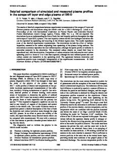
FIG. 1. Simulation box divided into 8 slabs along the X axis: 共a兲 the shading corresponds to temperature differences in the case of ‘‘thermal conductivity experiment’’ 共darker color indicates higher temperature兲 and 共b兲 the arrows indicate the average velocity in the slabs for the ‘‘shear viscosity experiment.’’
distribution functions of the particles. By the 400th 共for N ⫽8192) or 1000th time step 共for N⫽1024) the system was found to be perfectly thermalized and reached a steady temperature T 0 . At this time (t⫽t 0 ) a perturbation was applied to the system. For the thermal conductivity experiments the velocity of the particles was perturbed to obtain a sinusoidal spatial temperature profile 关 T(x) 兴 in the x direction. For the shear viscosity experiments the y component of the velocity of the particles was changed along the x direction. The simulation box was divided into 8 slabs along the X axis — as it is shown in Fig. 1 — and in each of these slabs a different temperature was set according to T 共 x k 兲 ⫽T 0 ⫹T M 0 sin
冉 冊
2xk , L
共7兲
where T M 0 is the amplitude of the temperature modulation and x k (k⫽1,2, . . . ,8) are the midpoints of the slabs along the X axis. At the time of the perturbation the total kinetic energy of the system was not changed. Similarly to this, in the case of shear viscosity ‘‘experiments’’ W 共 x k 兲 ⫽W M 0 sin
冉 冊
2xk , L
共8兲
was set, where W⫽ 具 v yi 典 i⫽1 . . . N , v yi being the y velocity component of the ith particle, and W M 0 is the amplitude of
Downloaded 09 Mar 2002 to 148.6.26.123. Redistribution subject to AIP license or copyright, see http://ojps.aip.org/pop/popcr.jsp
Phys. Plasmas, Vol. 7, No. 1, January 2000
Molecular dynamics calculation of the thermal . . .
47
the velocity modulation. Note that the average y velocity
具 v y 典 is zero before the modulation. The results reported here were obtained with 25% modulation depth, i.e., T M 0 /T 0 ⫽0.25 and W M 0 / 具 兩 v y 兩 典 ⫽0.25. After the modulation the T(x,t) temperature profile or the W(x,t) velocity profile was measured at each time step, a sinusoidal function was fitted to it, and its harmonic amplitude T M (t) or W M (t) was determined. The amplitudes of the modulation profiles T M (t) and W M (t) were found to fall exponentially for the experimental conditions discussed here, i.e., to follow the T 共 x,t 兲 ⫽T M 0 sin
冉 冊 冉
冊
t⫺t 0 2x exp ⫺ , L H
共9兲
solution of the one-dimensional heat-conductivity equation,
T 2T ⫽ , t c x2
共10兲
and in the case of ‘‘viscosity measurement’’ the W 共 x,t 兲 ⫽W M 0 sin
冉 冊 冉
2x t⫺t 0 exp ⫺ L S
冊
共11兲
solution of the shear viscosity equation,
v y 2v y , ⫽ t x2
共12兲
where c is the heat capacity, is the mass density, H and S are the characteristic times of the relaxation in the thermal conductivity and shear viscosity experiments, respectively. The transport coefficients can be calculated from the relaxation times as
冉 冊
⫽
c L H 2
⫽
L S 2
and
冉 冊
2
,
共13兲
.
共14兲
2
In Eq. 共10兲 the heat capacity at constant pressure is usually used. In our experiment, however, together with the temperature both the total internal energy 共U兲 and the pressure 共p兲 are spatially modulated 关see Eqs. 共3兲 and 共4兲兴. On the other hand, we have checked that the number of particles (N 1 ) did not change during the ‘‘experiments’’ in each of the slabs in the simulation box,29 i.e., the number density of the system can be considered homogenous 共neglecting the small spontaneous fluctuations兲. Thus the use of specific heat at constant volume (c v ) is appropriate in Eqs. 共10兲 and 共13兲. The specific heat c v of the OCP can be calculated as M c v⫽
冉 冊 U T
⫽Nk B V
冋
册
3 f 共⌫兲 ⫹ f 共 ⌫ 兲 ⫺⌫ , 2 ⌫
共15兲
where M is the mass of the system. Figure 2 illustrates the simulation method described above for the case of a thermal conductivity experiment. Figure 2共a兲 shows the T(x,t) – T 0 temperature distribution plotted for ⌫⫽3.9. Figure 2共b兲 displays the logarithm of the
FIG. 2. 共a兲 T(x,t) – T 0 temperature profile 共in K, averaged from four experiments兲 for ⌫⫽3.9 and N⫽8192. The modulation was applied at the 400th time step (t 0 ⬇12 ps兲. The modulation depth was 25%. 共b兲 Logarithm of the amplitude T M (t) as a function of time. The thick line is a linear fit to the data to illustrate the exponential decay of T M ; the slope gives the inverse of the relaxation time H .
T M (t) amplitude of the sinusoidal function fitted to T(x,t) – T 0 at each time step. The relaxation time H was determined by fitting a straight line to ln关TM(t)兴. It can be seen in Fig. 2共b兲 that ln关TM(t)兴 can be fitted by a straight line for a reasonable time interval. However, as T M decreases the fluctuations make the fitting more uncertain. Thus the fitting was executed for the time interval t 0 ⬍t⬍t 1 , where t 1 is defined by T M (t 1 )⫽T M (t 0 )/ ⑀ ( ⑀ ⫽2.718). The 25% modulation depth ensured T M (t 0 )⫽35 K at the time of modulation (t 0 ) and thus it gave ⬃10:1 signal to noise ratio 关in the measurement of T M (t)] which decreased at t⬎t 0 . Similar signal to noise ratio was found for the other values on ⌫ using the 25% modulation depth. The solutions of the heat-conductivity 共10兲 and shear viscosity 共12兲 equations, respectively, were obtained by assuming that and are independent of the temperature. The ‘‘experimentally’’ obtained exponential fall of T M (t) and W M (t) indicates that this is a reasonable approximation in
Downloaded 09 Mar 2002 to 148.6.26.123. Redistribution subject to AIP license or copyright, see http://ojps.aip.org/pop/popcr.jsp
48
Phys. Plasmas, Vol. 7, No. 1, January 2000
Z. Donko and B. Nyiri
the solution of 共10兲 and 共12兲. The assumption of a constant and would be more accurate at lower modulation depth (T M 0 /T 0 and W M 0 / 具 兩 v y 兩 典 ), however, we found that the 25% modulation depth was necessary so ensure that the modulation dominates over the spontaneous fluctuations. It is noted that for N⫽8192 a small positive drift of the system temperature (T 0 ) was observed in our simulations. This drift was most pronounced at low temperatures, it was 1%–2% over the relaxation time H 共or S ) at the highest ⌫ (⌫⬇20 for N⫽8192) and became even less important at higher temperatures. The drift 共which possibly originates from the unavoidable numerical errors in the simulations兲 could not be eliminated using shorter time steps. Using a smaller number of particles the drift decreased significantly and allowed us to study the OCP at ⌫ values as high as 125. This upper limit of ⌫ ensured that even at the 共25% deep兲 perturbation of the temperature all the parts of the system were still in the fluid state. III. RESULTS AND DISCUSSION
In this section the results of our calculations are presented and compared with previous results. We also discuss the limitations of our method. In the case of N⫽8192 four simulation runs were carried out for each value of ⌫ and the results and the error bars presented in the forthcoming figures represent the average and the standard deviation of the data obtained from the simulations. For N⫽1024 the number of runs was 72, first 9–9 runs were averaged; the results and error bars represent the average and standard deviation of 8 data values obtained this way. The standard deviation of the results ( ) ranges between 5% and 20% at the different values of ⌫. Figure 3共a兲 shows the relaxation times H and S obtained from our calculations for both system sizes (N ⫽1024 and 8192兲. The time units are given as the inverse of in Fig. 3. Our method is the plasma frequency P ⫽ ⫺1 P expected to yield correct transport coefficients when the relaxation time of the modulation profile ( H or S ) is much longer than the ‘‘local’’ thermalization time in the system. The speed of the local thermalization can be investigated by calculating the velocity autocorrelation function of the particles. Figure 3共b兲 shows the velocity autocorrelation function A vv ( )⫽ 具 v( )v(t 0 ⫹ ) 典 / 具 v(t 0 ) 2 典 共where 具典 denotes average over the particles兲 for different values of ⌫. The velocity autocorrelation time c 关defined as A vv ( c )⫽1/⑀ ; ⑀ ⫽2.718] is also plotted in Fig. 3共a兲 as a function of ⌫. It can be seen in Fig. 3共a兲 that with increasing ⌫ the velocity autocorrelation time C decreases as the collisions between the particles become more frequent and the information about the initial velocity of the particles is lost on a shorter time scale. At ⌫⭓20 the autocorrelation time is approximately constant, C / P ⬇2. At ⌫⬇1, in the system of 8192 particles the relaxation time of the temperature profile is H / P ⫽20.4, but in the system of 1024 particles it is only H / P ⫽7.7. This latter value is comparable to the velocity autocorrelation time C / P ⫽5.6. We found that this results in different values for the transport coefficients for different system sizes; in
FIG. 3. 共a兲 Relaxation times of the modulation profiles obtained in the thermal conductivity ( H ) and shear viscosity ( S ) ‘‘experiments’’ and velocity autocorrelation time defined as A vv ( c / p )⫽1/⑀ ( ⑀ ⫽2.718). p is the inverse of the plasma frequency. 共b兲 Velocity autocorrelation function A vv ( / p ) of the system for different values of ⌫.
smaller system lower values of and are obtained. With increasing ⌫ C decreases 关see Fig. 3共a兲兴 and the simulations give an increasing H and S . This behavior at ⌫⬇2 already results in an order of magnitude longer relaxation time compared to the velocity autocorrelation time. On the basis of this analysis we accepted the results for which the H / C ⭓10 or the S / C ⭓10 condition was fulfilled. The transport coefficients calculated taking into account this condition agreed within error bars for the different system sizes. Our previously calculated values of the thermal conductivity29 in the 1⭐⌫⭐2 range are however, most likely slightly underestimated. In the forthcoming figures the thermal conductivity and the shear viscosity are given in reduced units, *⫽
, nk B p a 2
共16兲
*⫽
, nm p a 2
共17兲
Downloaded 09 Mar 2002 to 148.6.26.123. Redistribution subject to AIP license or copyright, see http://ojps.aip.org/pop/popcr.jsp
Phys. Plasmas, Vol. 7, No. 1, January 2000
Molecular dynamics calculation of the thermal . . .
49
agree very well for all the calculations. At high values of ⌫ our results lie between the values of Vieillefosse and Hansen21 and those of Wallenborn and Baus.26 IV. SUMMARY
FIG. 4. Reduced thermal conductivity * of the classical 3D OCP as a function of ⌫. The thick line is a fit to the present results 共including both system sizes兲 in the 2⭐⌫⭐125 range.
where m is the mass of the particles and p is the plasma frequency, 2p ⫽ne 2 / 0 m. The thermal conductivity of the OCP as a function of ⌫ is shown in Fig. 4. The * values obtained by Bernu et al.27,28 are also displayed in Fig. 4. The stated accuracy of the results of Bernu et al. is 15%. Our results are consistent with the values given by these authors,27,28 though we obtained 20%–30% lower * . * exhibits a clear minimum in the ⌫⫽15– 20 range, as it was predicted previously.27,28 The results obtained for the reduced shear viscosity are presented in Fig. 5 together with the results of previous calculations. The best agreement is found between the present results and the molecular dynamics results of Bernu et al.27,28 Our results suggest that is ⬇20% – 30% higher that any previously accepted data in the ⌫⭐10 range. The * ⬇0.08 position of the minimum (⌫⬇20) and the value min
We carried out molecular dynamics experiments to determine the thermal conductivity * and shear viscosity * of the three-dimensional classical one-component plasma 共OCP兲. In our simulations the velocity of the particles was spatially modulated, and * and * were calculated from the relaxation time of the modulation profile. Based on the analysis of the velocity autocorrelation time of the particles, we found that our simulation method is valid in the 2⭐⌫ range. In this range of ⌫ the local thermalization of the particles is at least an order of magnitude faster than the relaxation of the modulation profiles applied to the system. The results presented here cover almost the entire fluid range of the OCP. The reduced shear viscosity * was found to exhibit a minimum at ⌫⬇20 in agreement with previous calculations. In the 2⭐⌫⭐10 range our method yields * values 20%– 40% higher compared to some of the previously obtained data, while very good agreement was found at the position of the minimum of * . The reduced thermal conductivity * exhibits a minimum similarly to * at ⌫⬇20. Our calculations resulted in 30%–40% lower thermal conductivity compared to previously accepted data. Our simulation method is not applicable below ⌫⬇2 with the present number of particles in the system. However, using N⬃105 – 106 particles reliable results could be expected for ⌫⭐1 values, as well. Finally it is noted that in principle the method would be applicable to calculate the bulk viscosity of the OCP. This could be done by applying a longitudinal velocity perturbation 共an x-dependent modulation of the v x velocity component兲. However, as the bulk viscosity is orders of magnitude lower than the shear viscosity, numerical difficulties are expected to arise using this method. ACKNOWLEDGMENTS
Helpful discussions with K. Ro´zsa, L. Szalai, and S. Hollo´ are gratefully acknowledged. This work was supported by the Hungarian Science Foundation Grant No. OTKA-T25989. M. Baus and J. P. Hansen, Phys. Rep. 59, 1 共1980兲. S. Ichimaru, Rev. Mod. Phys. 54, 1017 共1982兲. 3 S. Ichimaru, H. Iyetomi, and S. Tanaka, Phys. Rep. 149, 93 共1987兲. 4 H. M. Van Horn, Science 252, 384 共1991兲. 5 I. Yokoyama and S. Naito, Physica B 154, 309 共1989兲. 6 C. C. Grimes and G. Adams, Phys. Rev. Lett. 42, 795 共1979兲. 7 K. I. Golden, G. Kalman, and P. Wyns, Phys. Rev. A 46, 3463 共1992兲. 8 J. N. Tan, J. J. Bollinger, B. Jelenkovic´, and D. J. Wineland, Phys. Rev. Lett. 75, 4198 共1995兲. 9 W. M. Itano, J. J. Bollinger, J. N. Tan, B. Jelenkovic´, X.-P. Huang, and D. J. Wineland, Science 279, 686 共1998兲. 10 H. Thomas, G. E. Morfill, and D. Mohlmann, Phys. Rev. Lett. 73, 652 共1994兲. 1
2
FIG. 5. Reduced shear viscosity * of the classical 3D OCP as a function of ⌫. The thick line is a fit to the present results 共including both system sizes兲 in the 2⭐⌫⭐125 range.
Downloaded 09 Mar 2002 to 148.6.26.123. Redistribution subject to AIP license or copyright, see http://ojps.aip.org/pop/popcr.jsp
50 11
Phys. Plasmas, Vol. 7, No. 1, January 2000
W. L. Slattery, G. D. Doolen, and H. E. DeWitt, Phys. Rev. A 21, 2087 共1980兲. 12 S. G. Brush, H. L. Sahlin, and E. Teller, J. Chem. Phys. 45, 2102 共1966兲. 13 J. P. Hansen, Phys. Rev. A 8, 3096 共1973兲. 14 E. L. Pollock and J. P. Hansen, Phys. Rev. A 8, 3110 共1973兲. 15 H. Totsuji, Phys. Rev. A 17, 399 共1978兲. 16 R. C. Gann, S. Chakravarty, and G. V. Chester, Phys. Rev. B 20, 326 共1979兲. 17 S. Ogata and S. Ichimaru, Phys. Rev. A 36, 5451 共1987兲. 18 G. S. Stringfellow, H. E. DeWitt, and W. L. Slattery, Phys. Rev. A 41, 1105 共1990兲. 19 C. N. Likos and N. W. Ashcroft, Phys. Rev. Lett. 69, 316 共1992兲. 20 J. P. Hansen, I. R. McDonald, and E. L. Pollock, Phys. Rev. A 11, 1025 共1975兲. 21 P. Vieillefosse and J. P. Hansen, Phys. Rev. A 12, 1106 共1975兲.
Z. Donko and B. Nyiri R. W. Hockney and T. R. Brown, J. Phys. C 8, 1813 共1975兲. J. P. Hansen, D. Levesque, and J. J. Weis, Phys. Rev. Lett. 43, 979 共1979兲. 24 R. T. Farouki and S. Hamaguchi, Phys. Rev. E 47, 4330 共1993兲. 25 J. Wallenborn and M. Baus, Phys. Lett. A 61, 35 共1977兲. 26 J. Wallenborn and M. Baus, Phys. Rev. A 18, 1737 共1978兲. 27 B. Bernu, P. Vieillefosse, and J. P. Hansen, Phys. Lett. A 63, 301 共1977兲. 28 B. Bernu and P. Vieillefosse, Phys. Rev. A 18, 2345 共1978兲. 29 Z. Donko´, B. Nyı´ri, L. Szalai, and S. Hollo´, Phys. Rev. Lett. 81, 1622 共1998兲. 30 R. W. Hockney, S. P. Goel, and J. W. Eastwood, Chem. Phys. Lett. 21, 589 共1973兲. 31 R. W. Hockney and J. W. Eastwood, Comput. Phys. Commun. 19, 215 共1980兲. 32 R. W. Hockney and J. W. Eastwood, in Computer Simulation Using Particles 共McGraw–Hill, New York, 1981兲. 22 23
Downloaded 09 Mar 2002 to 148.6.26.123. Redistribution subject to AIP license or copyright, see http://ojps.aip.org/pop/popcr.jsp