PHYSICS OF PLASMAS
VOLUME 6, NUMBER 12
DECEMBER 1999
Onset of high-n ballooning modes during tokamak sawtooth crashes Y. Nishimura,a) J. D. Callen, and C. C. Hegna Department of Engineering Physics, University of Wisconsin-Madison, Madison, Wisconsin 53706-1687
共Received 27 July 1999; accepted 3 September 1999兲 A new phenomenon has been found during the nonlinear stage of the tokamak sawtooth crash in relatively high  plasmas. The m/n⫽1/1 magnetic island evolution gives rise to convection of the pressure inside the q⫽1 radius and builds up steep pressure gradient across the island separatrix, and thereby trigger ballooning instabilities below the threshold at the equilibrium. Effects of the ballooning modes on the magnetic reconnection process during the sawtooth crash are discussed. © 1999 American Institute of Physics. 关S1070-664X共99兲02812-8兴
I. INTRODUCTION
tion of the secondary high-n ballooning modes will be presented. Quantitative analysis of enhanced magnetic field line stochasticity is discussed in a separate paper.12 This paper is organized as follows. In Sec. II the basic model for magnetohydrodynamic 共MHD兲 simulation is discussed. In Sec. III, we present results of MHD simulations on the onset of high-n ballooning modes, showing evolution of both the pressure and magnetic field structures. Toroidal asymmetry of the m⫽1 magnetic island structure is discussed in Sec. IV. We summarize this work in Sec. V.
Sawtooth oscillations1 are generally observed in tokamak plasmas when the safety factor q at the magnetic axis is below unity. The temporally discontinuous soft x-ray signals suggest sudden electron temperature drops or crashes in the core of the plasma column. After the crash, the temperature profile inside the q⫽1 radius is flattened. 关Some exceptions of sawtooth free discharges are reported in Toroidal Experiment for Technically Oriented Research 共TEXTOR兲2 and Tokamak Fusion Test Reactor 共TFTR兲 supershots.3兴 There is a large gap between the theoretical understanding and the experimental results; the mechanism responsible for the nonlinear stage of the crash phase is far from being understood. The following two principal problems remain unsolved for sawtooth studies: 共1兲 The central q-value remains below unity during the crash in most experiments2 whereas zero-pressure Kadomtsev model predicts4 a full magnetic field reconnection and that the central q rises to above unity in the core of the plasma. 共2兲 The time scale of the final crash phase is much shorter than the one predicted by resistive reconnection4 or the Sweet–Parker layer model.5 In today’s high-temperature tokamak plasmas, the time scale is on the order of tens of microseconds.6 Recent experimental results, for example, those in Refs. 7 and 8, indicate dynamical temperature evolution during the crash phase of a sawtooth oscillation. Furthermore, the experimental measurements in TFTR6 have suggested the mode localization of the pressure driven modes 共ballooning modes兲 on the bad curvature side of the torus. On top of the ballooning mode localization, a series of TFTR experiments9,10 as well as TEXTOR experiments11 have inferred that the magnetic field line stochasticity in the vicinity of the q⫽1 radius plays an important role in thermal transport and the resultant rapid changes in the magnetic field structure. In the experiment,10 it is suggested that the pressure contours and the magnetic flux surface does not coincide during the nonlinearly developed stages of the crash. In this work, numerical simulation results on the excita-
II. BASIC MODEL FOR COMPUTATION
In this section, the basic properties of a magnetic field and a reduced MHD formulation in a tokamak are reviewed. A nonorthogonal, straight-field-line coordinate system is employed in the present calculations, in which is the flux surface label, is the poloidal-like angle, and is the toroidal angle. The magnetic field in a tokamak can be written as 共1兲
Beq⫽⫺Fⵜ ⫹ⵜ ⫻ⵜ eq ,
共2兲
˜ ⬅ⵜ⫻A ˜ ⫽ⵜ⫻ 共 ⫺ ˜ ⵜ 兲 ⫽ⵜ ⫻ⵜ ˜ , B
共3兲
where eq( ) and F( ) stand for the equilibrium poloidal magnetic flux and equilibrium poloidal current. Here, ˜ ( , , )⫽ 兺 m/n ˜ m/n ( )cos(m⫹n) is the poloidal flux function of the perturbed field, where m and n are the poloidal and the toroidal mode numbers, respectively. We denote the total poloidal magnetic flux as ( , , )⬅ eq( ) ⫹ ˜ ( , , ). Numerical simulation has been conducted employing a reduced MHD formulation13 in a toroidal geometry. Toroidal geometry enters via metric elements obtained from an equilibrium solver RSTEQ.14 The initial value simulation is conducted by employing the FAR code15 which originally contained a full set of MHD equations. In our study the reduced MHD equations13 are solved for the magnetic flux , the toroidal component of the vorticity U , and the pressure p. The relevant equations are: the toroidal component of Ohm’s law,
a兲
Present address: Department of Physics, University of Colorado, Boulder, Colorado 80309-0390. Electronic mail:
[email protected]
1070-664X/99/6(12)/4685/8/$15.00
˜, B⫽Beq⫹B
4685
© 1999 American Institute of Physics
Downloaded 06 Mar 2007 to 128.104.198.190. Redistribution subject to AIP license or copyright, see http://pop.aip.org/pop/copyright.jsp
4686
Phys. Plasmas, Vol. 6, No. 12, December 1999
⫽⫺R 2 关共 v⫻B兲 •ⵜ ⫺ J 兴 , t the vorticity equation,
冋 冉冊 冉
Nishimura, Callen, and Hegna
共4兲
冊 册
J  1 dU ⫹ 2 ⵜ ⫻ⵜ p •ⵜ ⫽S 2 R 2 B•ⵜ dt F 2⑀ B ⫹ ⬜ ⵜ 2 U ,
共5兲
and the pressure evolution equation, dp ⫽ ⬜ ⵜ⬜2 p. dt
共6兲
In these equations, R stands for the major radius, v⬅R 2 ⵜ ⫻ⵜ is the fluid velocity 共 is the stream function兲, U ⬅R 2 ⵜ⫻(R 2 v/F) is the vorticity, and J⬅ⵜ⫻B is the current density. Superscripts 共subscripts兲 denote the contravariant 共covariant兲 components. Here is the resistivity and the transport coefficients are given by ⬜ , and ⬜ , which are the perpendicular viscosity and the perpendicular heat conductivity, respectively. In this work heat conduction parallel to the magnetic field is ignored due to numerical difficulties. The maximum toroidal beta value at the magnetic axis is denoted by , while the inverse aspect ratio is ⑀. The reduced MHD formulation is derived by neglecting ⑀ 2 and higherorder terms and is correct to the small inverse aspect ratio limit where ⑀Ⰶ1. Time is normalized by the resistive time r ⬅a 2 / and the length is normalized by the minor radius a. The Lundquist number is given by S⬅ r / a where a is the poloidal Alfven transit time. Incompressibility (ⵜ•R ⫺2 v⫽0) is implicit in Eq. 共6兲. Toroidal curvature effects are included in the second term of Eq. 共5兲, which is the minimum requirement to describe the ballooning-type pressure driven modes. The reduced MHD does not precisely include the effect of the n⫽1 toroidal internal kink mode. The analysis by Bussac et al.16 reveals that the mode enters through order ⑀ 4 in the variational principle.16 Bussac et al.16 have shown that the internal kink mode is only unstable when  p,Bussac⬎0.3 (  p,Bussac is the poloidal beta value which is volume averaged within the q⫽1 radius, and differs from the conventional poloidal beta  p ). In our simulation, possibly due to the absence of higher-order term effects, the m/n⫽1/1 ideal/ resistive kink modes are always linearly unstable regardless of what  value one employs. To time advance the reduced MHD equations, the unknown quantities x( , , ) in Eqs. 共4兲, 共5兲, and 共6兲 are separated into equilibrium and perturbation parts: x( , , ) ˜ ( , , ). The purely equilibrium terms are dis⫽x eq( , )⫹x carded in the FAR code,15 leaving only terms that are linear or quadratic in the perturbed quantities. Linear calculations ˜ terms implicitly, while nonlintime advance only the x eq⫻x ˜ explicitly. ear calculations integrate quadratic terms ˜x ⫻x ˜ The perturbed quantities x ( , , ) are finite differenced in and expanded in Fourier series for the poloidal angle and the toroidal angle . At t⫽0 we perturb a single resonant mode 1/1 with a finite amplitude. To see the evolution of
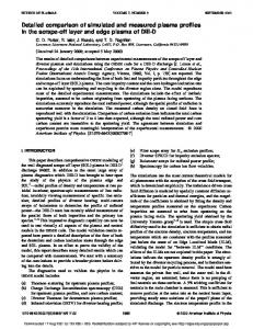
FIG. 1. Mode spectrum employed for the simulation. The abscissa and ordinate corresponds to poloidal and toroidal mode numbers, respectively. A total of 151 modes are used in the simulations.
magnetic structures, magnetic field line trajectories have been obtained by integrating the magnetic field line equation d B 1 ⫽ ⫽⫺ , d B F 1 d B ⫽ ⫽ , d B F using a fourth-order Runge–Kutta–Gill method.17 III. SIMULATION RESULTS
Parameters used in the calculations were as follows. The q-profile is taken as a peaked profile.18 The central-q is taken as q 0 ⫽0.81 to avoid the resonance of m/n⫽4/5 mode near the magnetic axis. The equilibrium pressure profile has the 2 form of p⫽ eq . Major radius R⫽5 m, minor radius a ⫽1.25 m 共the inverse aspect ratio ⑀⫽1/4兲, and Lundquist number S⫽105 are taken. A total of 500 equally spaced mesh points was used in the radial direction. The mode spectrum was selected as shown in Fig. 1, so that it fills the 0.81⭐q⬃m/n⭐2.7 region. A total of 151 modes was included in the simulations. The transport coefficients are taken as small as possible: ⬜ ⫽0.1, and ⬜ ⫽0.1. Figures 2共a兲 and 2共b兲 show pressure contours in the poloidal cross sections at ⫽ and ⫽0 after a nonlinear evolution of m⫽1 magnetic island. All the figures in this paper are plotted in the Cartesian 共configuration space兲 coordinates (X,Z). The center line of the torus is located at the middle of the figure and the toroidal magnetic field falls off proportional to 1/R toward the edges. In Fig. 2,  of 4% 共poloidal beta of  p ⫽0.74) was used. The green and yellow crescentshaped part corresponds to the magnetic island. Localization of the mode on the bad curvature side can be seen starting from t⫽1.205⫻10⫺2 ; the m/n⫽1/1 magnetic island evolution gives rise to convection of the pressure inside the q ⫽1 radius and builds up a steep pressure gradient across the
Downloaded 06 Mar 2007 to 128.104.198.190. Redistribution subject to AIP license or copyright, see http://pop.aip.org/pop/copyright.jsp
Phys. Plasmas, Vol. 6, No. 12, December 1999
Onset of high-n ballooning modes during tokamak . . .
4687
FIG. 2. Pressure contours for the ⫽4% simulation. The axisymmetry center line is located at the middle of the page. 共a兲, 共b兲 at t⫽1.205⫻10⫺2 , 共c兲, 共d兲 at t⫽1.230⫻10⫺2 , and 共e兲, 共f兲 at t⫽1.265⫻10⫺2 .
island separatrix or the Y-ribbon,19 and thereby triggers ballooning instabilities below the threshold at the equilibrium. At later times (t⫽1.230⫻10⫺2 and t⫽1.265⫻10⫺2 ), typical ballooning type structures 共so-called ballooning fingers兲 on the bad curvature side can be seen. Note that the corresponding high-n mode activity is suppressed in Figs. 2共a兲, 2共c兲, and 2共e兲 where the hot core is facing the good curvature side. Figures 2共e兲 and 2共f兲 show the final temperature crash phase. Figure 3 shows eigenprofiles of the streamfunction : the commensurate 1/1 to 10/10 mode spectrum, at t⫽1.175 ⫻10⫺2 when the high-n mode amplitudes are small, and at t⫽1.230⫻10⫺2 when the high-n modes are active. Figure 3 indicates rapid growth of the 8/8 to 10/10 modes 共red, blue, and green curves兲. Figure 4 shows eigenprofiles of n⫽10 modes but with different m 共poloidal mode兲 numbers. These incommensurate helicity modes grow simultaneously. This is a typical eigenmode structure of ballooning modes; different m modes with same n are correlated in the ballooning transformation.20 Note that each of the modes are localized near the corresponding mode rational surfaces exhibiting the nature of Weber functions21— say 15/10 at q⫽1.5 surface 共red兲, 16/10 at q⫽1.6 共blue兲, 17/10 at q⫽1.7 共green兲 . . . , and so on.
FIG. 3. Fourier spectrum of the stream functions 共a兲 at t⫽1.175⫻10⫺2 and 共b兲 at t⫽1.230⫻10⫺2 . Commensurate modes, m/n⫽1/1 to m/n ⫽10/10.
An important observation is that these higher number modes are not active in the axisymmetric equilibrium but are triggered by the change in the pressure profile in the vicinity of the Y-ribbon.19 These high-n modes are not generated from mode coupling but rather they result from changes in the n⫽0 equilibrium modes. The ideal n⫽10 ballooning modes are stable to ⬃⑀ which is allowed for the reduced MHD description.13 The resistive ballooning modes22 are always unstable with a linear growth rate proportional to S ⫺1/3 共here, S is the Lundquist number兲, just as for the m/n⫽1/1 resistive kink mode. However, in our simulation model, the small amplitudes of n⫽10 modes at t⫽0 never catch up with the amplitude of m/n⫽1/1 mode, unless there is a triggering mechanism such as pressure steepening across the island separatrix. The phenomena is different from a mode-
Downloaded 06 Mar 2007 to 128.104.198.190. Redistribution subject to AIP license or copyright, see http://pop.aip.org/pop/copyright.jsp
4688
Phys. Plasmas, Vol. 6, No. 12, December 1999
Nishimura, Callen, and Hegna
FIG. 5. The velocity field for the ⫽4% simulation. The axisymmetry center line is located at the middle of the page. 共a兲, 共b兲 at t⫽1.205⫻10⫺2 , 共c兲, 共d兲 at t⫽1.230⫻10⫺2 , and 共e兲, 共f兲 at t⫽1.265⫻10⫺2 . The lengths of the arrows are in the same unit for all the figures.
FIG. 4. Fourier spectrum of stream function 共a兲 At t⫽1.175⫻10⫺2 and 共b兲 at t⫽1.230⫻10⫺2 . All modes shown have the same toroidal mode number n⫽10, but they have incommensurate helicities.
coupling energy cascade as one sees in magnetoturbulence.23,24 Figure 5 shows the flow velocity field for the same ⫽4% simulation. Interestingly, we can observe small scale eddy structures along the ballooning mode fingers streaming both inward and outward. Note that the significant eddy appears outside the q⫽1 radius, while similar structures exist inside the q⫽1 radius. These eddies convect plasma substantial distances across the q⫽1 surfaces. In an actual plasma discharge, no modes can keep growing forever, unless, say, the entire plasma discharge is terminated. Any instability should reach a saturation stage. For example, in Fig. 2共f兲 the ballooning mode fingers are torn and we see a transition to another instability perhaps of a Kelvin–Helmholtz type.25 This signifies that numerous m/n
⫽1/1 modes come into play and destroy the coherent structures. A key to understand ‘‘tearing’’ of the ballooning fingers is the finite dissipation. In a dissipative plasma, resistivity as well as viscosity plays a role in damping modes, especially in the short wavelength modes. As a reminder, the diffusion terms in Eqs. 共5兲 and 共6兲 are proportional to m 2 . Figure 6 shows magnetic field line Poincare´ plots during the ballooning mode evolution, at the time corresponding to those for the pressure contours of Fig. 2. As one can see, although the magnetic field lines are globally stochasticized, the field lines basically follow pressure surfaces. This is in contrast to the work by Kleva and Guzdar26 where the authors claim that the pressure and the magnetic field completely decouple and the pressure finger evolution does not affect the poloidal magnetic field strength. From the numerical measurement of the local magnetic field line pitch at t⫽1.265⫻10⫺2 we obtained q 0 ⬍1 near the shifted magnetic axis. The value of q-profiles for both the equilibrium 共the solid line兲 and at the time t⫽1.265⫻10⫺2 共circles兲 are shown in Fig. 7. Given the location of the shifted magnetic axis (X 0 ,Z 0 ) in a Cartesian coordinate system, a poloidal angle is calculated from
Downloaded 06 Mar 2007 to 128.104.198.190. Redistribution subject to AIP license or copyright, see http://pop.aip.org/pop/copyright.jsp
Onset of high-n ballooning modes during tokamak . . .
Phys. Plasmas, Vol. 6, No. 12, December 1999
4689
FIG. 7. The safety factor profile at the equilibrium 共solid line兲 and at t ⫽1.265⫻10⫺2 共circles兲 which corresponds to Fig. 6共f兲.
FIG. 6. Poincare´ plots of magnetic field line trajectories for the ⫽4% simulation. The axisymmetry center line is located at the middle of the page. 共a兲, 共b兲 at t⫽1.205⫻10⫺2 , 共c兲, 共d兲 at t⫽1.230⫻10⫺2 , and 共e兲, 共f兲 at t ⫽1.265⫻10⫺2 .
⌰⫽arctan
Z⫺Z 0 共 兲 . X⫺X 0 共 兲
Then, the safety factor is calculated by an averaged field line pitch
具 q 典 ⫽ lim
→⬁
. ⌰ 共 兲 ⫺⌰ 共 0 兲
共7兲
The averaged 具 q 典 -value in the perturbed state is no more than the ratio between the number of toroidal windings to poloidal windings. In Fig. 7, only five toroidal evolutions were taken for in Eq. 共7兲. If one follows field lines for a long period, the information of the initial position is lost due to magnetic stochasticity. In Figs. 6共c兲–6共f兲, global stochasticity can be seen in the annular region extending to q⬃2 共most of the flux surface except for a few peripheral regions are destroyed兲. The q ⫽1 annular region is stochastic enough to produce rapid radial heat transport. 共Note that parallel heat conduction is taken as zero in the work of this paper.兲 A simultaneous excitation of incommensurate high-n modes and the island overlapping allows rapid escape of the heat from the center to the q⭓1 regions. This mode coupling feature of the bal-
looning modes and resultant global stochasticity can be a possible explanation for the rapid escape of the heat observed in TFTR experiment.10 As a result, after the stage of Figs. 2共e兲 and 2共f兲, the effect of finite parallel heat transport along the stochastic magnetic field lines becomes dominant for the pressure evolution. The inclusion of parallel heat transport effects into the MHD model is numerically too demanding and we do not present these simulation results in this paper. With a decrease in  共4%→2%, see Fig. 8兲, the ballooning structures can be still seen, but they are rather modest (  p ⫽0.49 for ⫽2%兲. The onset of the ballooning instability is delayed for this lower  case; finger-like structures appear at a much later phase of the m⫽1 island evolution. It takes a longer time for the pressure gradient to build up to the ballooning threshold. Another observation is the degree of radial extension of the fingers. In the ⫽2% case, the finger extends only up to q⬃1.3 surface. As a result, the extension of stochastic annular region is modest compared to higher  cases. Figure 9 shows magnetic field line Poincare´ plots during the ballooning mode evolution, at the time corresponding to those for the pressure contours of Fig. 8. In the lower  (  p ⬍0.25) limit, the magnetic field lines seem to recover the Kadomtsev-type full magnetic reconnection. As a reminder, the TEXTOR11 experiments are conducted in  p ⭐0.3 and the work by Nagayama et al. in TFTR6 experiments reveals  p ⬃0.95 for the hot ion mode,  p ⬃0.4 for the ion cyclotron range of frequencies 共ICRF兲 plasmas, and  p ⬃0.11 for the Ohmic plasmas. Although magnetic stochasticity induced by the ballooning modes may play a role, the mechanism for the incomplete magnetic reconnection process in the low- plasmas remains to be explored. IV. TOROIDAL ASYMMETRY OF THE m ⴝ1 MAGNETIC ISLAND
For the simulation in this section, we have taken the equilibrium q profile and the pressure profile 共the equilib-
Downloaded 06 Mar 2007 to 128.104.198.190. Redistribution subject to AIP license or copyright, see http://pop.aip.org/pop/copyright.jsp
4690
Phys. Plasmas, Vol. 6, No. 12, December 1999
Nishimura, Callen, and Hegna
FIG. 8. Pressure contours for the ⫽2% simulation. The axisymmetry center line is located at the middle of the page. 共a兲, 共b兲 at t⫽1.162⫻10⫺2 , 共c兲, 共d兲 at t⫽1.187⫻10⫺2 , and 共e兲, 共f兲 at t⫽1.225⫻10⫺2 .
FIG. 9. Poincare´ plots of magnetic field line trajectories for the ⫽2% simulation. The axisymmetry center line is located at the middle of the page. 共a兲, 共b兲 at t⫽1.162⫻10⫺2 , 共c兲, 共d兲 at t⫽1.187⫻10⫺2 , and 共e兲, 共f兲 at t⫽1.225⫻10⫺2 .
rium of ⫽4%兲 as in the previous section. However, we do not include pressure/curvature effects in the mode evolution and we set ⫽0 in Eq. 共5兲. Thus, the plasma responds to a Shafranov shift 共which is 17% of the minor radius for the equilibrium employed here兲 and the equilibrium geometry metric elements, but the dynamical ballooning mode evolution is absent. The aim of this rather artificial calculation is to extract the magnetic field line structure near the m⫽1 island separatrix or the current sheet, until the moment of the ballooning modes onset. As shown in Figs. 6 and 9, once the short wavelength ballooning modes are triggered, the magnetic field lines basically follow the pressure surface which exhibits the finger-like structure. As suggested by Hegna and Callen27 the local magnetic shear can be an important factor for the triggering of ballooning modes. The ballooning modes can become unstable when the destabilizing pressuredrive overcomes the field line bending stabilizing contribution on the perturbed magnetic surface.27 Inclusion of a dynamical curvature term generates magnetic stochasticity and makes observation of the magnetic structures very difficult. Here, we have also employed an extremely large viscosity value ( ⬜ ⫽5.0) so as to kill the strong flow. Figure 10 shows Poincare´ plots of magnetic field line trajectories when the hot core is facing the good 共left兲 and
the bad 共right兲 curvature sides of the plasma. As before, the center line is located at the middle of the figure, and the toroidal magnetic field falls off as ⬃1/R from the center toward edges of the figure. By comparing Poincare´ mappings of the field line trajectories on the good and bad curvature sides, toroidal asymmetry in the magnetic field structure can be seen: the internal column is close to the wall in Fig. 10共b兲 when the hot core region faces the bad curvature side. One can observe the three-dimensional structure of the current sheet28 of the m⫽1 magnetic island 共or the Y-ribbons19兲; the compression of the flux surfaces is much more pronounced at a toroidal angle where the current sheet is located on the bad curvature side of the torus. The central core has an oval shape rather than circular. The oval shape is upright when facing the bad curvature side, but horizontal when facing the good curvature side. As shown in Figs. 10共e兲 and 10共f兲, Kadomtsev-type full magnetic reconnection4 takes place in the absence of dynamical ballooning modes. From this magnetic structure, one can expect that the resultant ballooning-type instabilities across the q⫽1 surface will be toroidally localized by their alignment with the magnetic island structure. This mechanism is not the same as the localization of the ballooning modes which is demonstrated in the previous section. This mechanism arises from the geo-
Downloaded 06 Mar 2007 to 128.104.198.190. Redistribution subject to AIP license or copyright, see http://pop.aip.org/pop/copyright.jsp
Phys. Plasmas, Vol. 6, No. 12, December 1999
FIG. 10. Poincare´ plots of magnetic field line trajectories for the ⫽4% simulation. Kadomtsev type full reconnection takes place in the absence of dynamical ballooning modes. The axisymmetry center line is located at the middle of the page. 共a兲, 共b兲 at t⫽2.52⫻10⫺2 , 共c兲, 共d兲 at t⫽2.56⫻10⫺2 , and 共e兲, 共f兲 at t⫽2.60⫻10⫺2 .
metrical effects on the m/n⫽1/1 magnetic island evolution due to the 1/R dependence of the toroidal magnetic field.
V. SUMMARY AND DISCUSSION
In this paper, the tokamak sawtooth crash phase has been studied numerically employing a toroidal magnetohydrodynamic initial value simulation. Motivated by experimental results from TFTR showing dramatic temperature evolution during the crash, emphasis has been put on the role of pressure driven high-n ballooning modes. With a wide selection of Fourier modes, it has been shown that the m/n⫽1/1 magnetic reconnection process induces nonlinearly unstable high-n ballooning modes; the m/n⫽1/1 magnetic island modifies the pressure profiles and generates unstable states for ballooning modes. The ballooning spectrum in the simulation compares favorably with that expected from conventional MHD theory;20 all the modes with different m numbers but with the same n mode numbers are correlated. In the crash phase, it is observed that small scale vortices are generated. The results were significant in suggesting the breaking of the symmetric m⫽1 flows, and
Onset of high-n ballooning modes during tokamak . . .
4691
hence the possibility of temperature profile flattening without complete magnetic reconnection in tokamak plasma discharges. As an artificial probe for the onset mechanism of high-n ballooning modes, the m/n⫽1/1 island evolution for a large equilibrium  value 共and thus a large Shafranov shift兲 has been simulated but without the dynamical pressure-drive. By comparing the magnetic field line trajectories on the good and bad curvature sides, we have observed a threedimensional, non-axisymmetric structure of the m⫽1 magnetic island. It has been shown that the current sheet,28 or the Y-ribbon,19 is stretched 共vertically elongated兲 when it is facing the bad curvature side. The effect is considered to induce ballooning modes on the bad curvature side. Compared to previous work by Park et al.29 where the helically twisted equilibrium produced by the kink mode was taken as an initial configuration, this is the first MHDsimulation to reveal the activity of the secondary high-n ballooning modes, starting from a self-consistent concentric equilibrium that evolved into an m/n⫽1/1 magnetic island structure. The simulation by Park et al.29 was conducted to account for the TFTR  limit disruptions30 rather than sawtooth crashes. In the  limit disruptions30 it is observed that the ideal kink modes 共instead of resistive kink modes兲 give rise to precursor signals and the 1/1 kink strongly couples to higher m/n components. 共It is worth pointing out that the localization of a pressure hot bulge to the bad curvature side during the m/n⫽1/1 island evolutions has been demonstrated by Park et al.31 and Aydemir.32兲 To emphasize again, in our studies, the high-n ballooning activity does not come from the mode couplings. The ballooning modes are suddenly triggered due to the emergence of the magnetic island or the ‘‘topological change in magnetic field lines’’ and the local pressure steepening. With regard to magnetic structures, it has been shown that the ballooning mode can break the helical symmetry and thereby induce magnetic stochasticity. In the high- simulations, significant stochasticity has been induced by the strong mode couplings between modes of incommensurate helicity, which can induce radial thermal transport along the field lines. This supports TFTR experimental results which suggest rapid heat escape from the center to the outside q⫽1 region.10 The relation of our simulation results to the experimentally observed partial reconnection in TFTR6 is discussed here. As indicated experimentally10 the flattening of the temperature profile takes place before the full reconnection of the magnetic field lines. We suggest that, in relatively high- plasmas, the ballooning modes are playing a role in the flattening of the temperature crash in the nonlinear stage of sawtooth events. The dominant mode is converted from the m/n⫽1/1 mode to n⫽10 higher harmonics 共via onset of high-n ballooning modes兲. Furthermore, we conjecture that the resultant small scale vortices may be playing an important role in the mixing and at the same time damping of strong m⫽1 flow. At the temperature crash phase, we have shown that the local magnetic field line pitch at the magnetic axis stays as q 0 ⬍1. Though the parallel heat transport along the stochastic magnetic field lines becomes dominant for the
Downloaded 06 Mar 2007 to 128.104.198.190. Redistribution subject to AIP license or copyright, see http://pop.aip.org/pop/copyright.jsp
4692
Phys. Plasmas, Vol. 6, No. 12, December 1999
pressure evolution after the temperature crash, we did not simulate the effect in this paper. The heat conduction effects parallel to the magnetic field lines remain to be explored, since, in the lower  limit (  p ⭐0.25), our simulation results seem to recover the Kadomtsev type full magnetic reconnection, while the experimental results from TEXTOR11 and TFTR10 typically reveal the partial magnetic reconnection. The experimental sawteeth analyses by Nagayama et al.6 exhibit the localization of the ballooning modes on the bad curvature side in high- TFTR discharges. Our simulation results of ballooning mode in high  共⬎2% and  p ⬎0.49) have common features with their experimental findings. On the other hand, as shown in Figs. 6 and 9, the magnetic topology at the both sides of the torus seems to be the same, and did not reveal the evidence of threedimensional reconnection model proposed by Nagayama et al.6 We suspect this discrepancy can be due to the reduced MHD formulation we employed and the lack of stabilizing parallel heat transport effects along stochastic magnetic field lines 共the possibility of the three-dimensional reconnection process still remains兲. Collisionless magnetic reconnection model has been developed33,34 to explain fast reconnection including nonideal kinetic effects in the thin current layer. Our numerical simulation results are antithetical to those models in that high-n ballooning modes across the current layer can destroy effects such as electron inertia. It is difficult to imagine that the electron current sheet is not being influenced by the pressure-drive effects which cause very strong radial flows. As a summary, this paper has demonstrated an important nature of the high-n, m/n⫽1/1 mode activities during the tokamak sawtooth crash in relatively high- plasmas. We further investigated the strong interaction between the m ⫽1 flow and the high-n mode flows. Further progress in the magnetic reconnection model will be reported in the future. ACKNOWLEDGMENTS
One of the authors 共YN兲 is grateful to Dr. B. Coppi, Dr. Y. Nagayama, Dr. W. Park, and Dr. M. Yamada for valuable suggestions. Y.N. would like to acknowledge an enormous credit from Dr. B. A. Carreras, Dr. L. A. Charlton, Dr. H. R. Hicks, Dr. J. A. Holmes, Dr. J-N. G. Leboeuf, Dr. D. K. Lee, Dr. V. E. Lynch, Dr. D. A. Spong, and Dr. B. V. Waddell for the development of FAR. This research was supported by United States Department of Energy Grant No. DE-FG02-86ER53218. 1
S. von Goeler, W. Stodiek, and N. Sauthoff, Phys. Rev. Lett. 33, 1201 共1974兲. 2 H. Soltwisch, W. Stodiek, J. Manickam, and J. Schlu¨ter, in Plasma Physics and Controlled Nuclear Fusion Research, 1986, Proceedings of the 11th International Conference, Kyoto 共International Atomic Energy Agency, Vienna, 1987兲, Vol. 1, p. 263; H. Soltwisch, Rev. Sci. Instrum. 59, 1599 共1988兲.
Nishimura, Callen, and Hegna 3
F. M. Levinton, L. Zakharov, S. H. Batha, J. Manickam, and M. C. Zarnstorff, Phys. Rev. Lett. 72, 2895 共1994兲. 4 B. B. Kadomtsev, 1, 389 共1975兲; B. B. Kadomtsev, in Plasma Physics and Controlled Nuclear Fusion Research, 1976, Proceedings of the 6th International Conference, Berchtesgaden 共International Atomic Energy Agency, Vienna, 1977兲, Vol. 1, p. 555. 5 E. N. Parker, Astrophys. J. 121, 491 共1955兲; P. A. Sweet, Nuovo Cimento Suppl. 8, 188 共1958兲. 6 Y. Nagayama, M. Yamada, W. Park, E. D. Fredrickson, A. C. Janos, K. M. McGuire, and G. Taylor, Phys. Plasmas 3, 1647 共1996兲. 7 Y. Nagayama, K. M. McGuire, M. Bitter, A. Cavallo, E. D. Fredrickson, K. W. Hill, W. Park, G. Taylor, and M. Yamada, Phys. Rev. Lett. 67, 3527 共1991兲. 8 J. D. Callen, B. A. Carreras, and R. D. Stambaugh, Phys. Today 45, 34 共1992兲. 9 E. D. Fredrickson, K. McGuire, A. Cavallo, R. Budny, A. Janos, D. Monticello, Y. Nagayama, W. Park, G. Taylor, and M. C. Zarnstorff, Phys. Rev. Lett. 65, 2869 共1990兲. 10 M. Yamada, F. Levinton, N. Pomphrey, R. Budny, J. Manickam, and Y. Nagayama, Phys. Plasmas 1, 3269 共1994兲. 11 H. Soltwisch and H. R. Koslowski, Plasma Phys. Controlled Fusion 37, 667 共1995兲. 12 Y. Nishimura, Ph.D. dissertation, University of Wisconsin–Madison, 1998. 13 H. R. Strauss, Phys. Fluids 20, 1354 共1977兲. 14 V. E. Lynch, B. A. Carreras, H. R. Hicks, J. A. Holmes, and L. Garcia, Comput. Phys. Commun. 24, 465 共1981兲. 15 L. A. Charlton, J. A. Holmes, H. R. Hicks, V. E. Lynch, and B. A. Carreras, J. Comput. Phys. 63, 107 共1986兲. 16 M. N. Bussac, R. Pellat, D. Edery, and J. L. Soule, Phys. Rev. Lett. 35, 1638 共1975兲. 17 M. Abramowitz and I. A. Stegun, Handbook of Mathematical Functions 共Dover, New York, 1970兲, p. 896. A better fourth order Runge–Kutta– Gill method which includes corrections to the truncation error can be found in I. Kawakami, Suuchi-keisan 共Iwanami, Tokyo, 1989兲, p. 159 共in Japanese兲. 18 H. P. Furth, P. H. Rutherford, and H. Selberg, Phys. Fluids 16, 1054 共1973兲. 19 F. L. Waelbroeck, Phys. Fluids B 1, 2372 共1989兲. 20 J. W. Connor, R. J. Hastie, and J. B. Taylor, Phys. Rev. Lett. 40, 396 共1978兲. 21 M. Abramowitz and I. A. Stegun, Handbook of Mathematical Functions 共Dover, New York, 1970兲, p. 498. 22 R. B. White, Theory of Tokamak Plasmas 共North-Holland, Amsterdam, 1989兲, p. 192. 23 D. Biskamp, Nonlinear Magnetohydrodynamics 共Cambridge, London, 1993兲, p. 183. 24 K. Hallatschek, A. Gude, D. Biskamp, S. Gu¨nter, and ASDEX Upgrade Team, Phys. Rev. Lett. 80, 293 共1998兲. 25 S. Chandrasekhar, Hydrodynamic and Hydromagnetic Stability 共Clarendon, Oxford, 1961兲, p. 507. 26 R. G. Kleva and P. N. Guzdar, Phys. Rev. Lett. 80, 3081 共1998兲. 27 C. C. Hegna and J. D. Callen, Phys. Fluids B 4, 3031 共1992兲. 28 M. N. Rosenbluth, R. Y. Dagazian, and P. H. Rutherford, Phys. Fluids 16, 1894 共1973兲. 29 W. Park, E. D. Fredrickson, A. Janos, J. Manickam, and W. M. Tang, Phys. Rev. Lett. 75, 1763 共1995兲. 30 E. D. Fredrickson, K. McGuire, Z. Chang, A. Janos, M. Bell, R. V. Budny, C. E. Bush, J. Manickam, H. Mynick, R. Nazikian, and G. Taylor, Phys. Plasmas 2, 4216 共1995兲. 31 W. Park, D. A. Monticello, E. D. Fredrickson, and K. McGuire, Phys. Fluids B 3, 507 共1991兲. 32 A. Aydemir, Phys. Fluids B 2, 2135 共1990兲. 33 J. A. Wesson, Nucl. Fusion 30, 2545 共1990兲. 34 D. Biskamp and J. F. Drake, Phys. Rev. Lett. 73, 971 共1994兲.
Downloaded 06 Mar 2007 to 128.104.198.190. Redistribution subject to AIP license or copyright, see http://pop.aip.org/pop/copyright.jsp