Using PHP format

PHYSICS OF PLASMAS

VOLUME 7, NUMBER 10

OCTOBER 2000

Experimental study of the bifurcation nature of the electrostatic potential of a toroidal helical plasma A. Fujisawa, H. Iguchi, T. Minami, Y. Yoshimura, K. Tanaka, K. Itoh, H. Sanuki, S. Lee, M. Kojima,a) S.-I. Itoh, M. Yokoyama, S. Kado, S. Okamura, R. Akiyama, K. Ida, M. Isobe, S. Nishimura, M. Osakabe, I. Nomura, A. Shimizu, C. Takahashi, K. Toi, K. Matsuoka, Y. Hamada, and M. Fujiwara National Institute for Fusion Science, Oroshi-cho, Toki, 509-5292 Japan

共Received 28 March 2000; accepted 6 July 2000兲 The bifurcation nature of the electrostatic structure is studied in the toroidal helical plasma of the Compact Helical System 共CHS兲关K. Matsuoka et al., Proceedings of the 12th International Conference on Plasma Physics and Controlled Nuclear Fusion Research, Nice, 1988 共International Atomic Energy Agency, Vienna, 1989兲, Vol. 2, p. 411兴. Observation of bifurcation-related phenomena is introduced, such as characteristic patterns of discrete potential profiles, and various patterns of self-sustained oscillations termed electric pulsation. Some patterns of the electrostatic structure are found to be quite important for fusion application owing to their association with transport barrier formation. It is confirmed, as is shown in several tokamak experiments, that the thermal transport barrier is linked with electrostatic structure through the radial electric field shear that can reduce the fluctuation resulting in anomalous transport. This article describes in detail spatio-temporal evolution during self-sustained oscillation, together with correlation between the radial electric field and other plasma parameters. An experimental survey to find dependence of the temporal and spatial patterns on plasma parameters is performed in order to understand systematically the bifurcation property of the toroidal helical plasma. The experimental results are compared with the neoclassical bifurcation property that is believed to explain the observed bifurcation property of the CHS plasmas. The present results show that the electrostatic property plays an essential role in the structural formation of toroidal helical plasmas, and demonstrate that toroidal plasma is an open system with a strong nonlinearity to provide a new attractive problem to be studied. © 2000 American Institute of Physics. 关S1070-664X共00兲04310-X兴

I. INTRODUCTION

issue to address is how the structure of the radial electric field is related to plasma transport.11–15 A number of theoretical and experimental works have been devoted to clarification of the relationship between transport and the structure of radial electric field. In the Continuous Current Tokamak 共CCT兲 and Tokamak Experiment for Technically Oriented Research 共TEXTOR兲,16,17 the radial electric field generated with a biasing electrode at the plasma edge successfully induced forced H-mode transitions. The impact of the radial electric field on transport began to become widely noticed. Following confirmation of the edge transport barrier in other tokamak experiments, similar improved confinement regimes were also found in two toroidal helical plasmas, the Wendelstein7-AS and Compact Helical System 共CHS兲.18,19 Before these findings, bifurcation of the radial electric field had been expected in toroidal helical plasmas by a neoclassical theory including helical ripple diffusion.20–22 In contrast to tokamaks, the neoclassical theory had predicted that the absolute value of the radial electric field affected the transport in toroidal helical plasmas. The radial electric field, therefore, had been a primary physical quantity in toroidal helical plasmas, even without the discovery of the H-mode. At present, the radial electric field of the interior is received attention as a key to determine the global property of toroidal

Plasma is a matter of non-thermoequilibrium with strong nonlinearity. Its structural formation could be one of the most attractive issues as a general physics subject,1 similar to dissipative structures, such as the Be´rnard cell, BelouzovZhabotinskii 共BZ兲 reaction and so on. A bifurcation property of toroidal plasmas is recognized for the first time in the Axisymmentrical Divertor Experiment 共ASDEX兲 tokamak.2 There the plasma suddenly changes from so-called L-mode into H-mode as the auxiliary heating power is increased. The H- and L-modes are characterized by high and low plasma confinement, respectively, or the H-mode is equivalent to the formation of edge transport barrier associated with suppression of fluctuation-driven transport.3,4 This discovery is important in terms of fusion application, as well as physics interest, since this could give a more economical way to achieve a high plasma performance. A predominant working hypothesis to explain this spontaneous change of plasma property is based on bifurcation in the radial electric field or plasma rotation velocity.5–7 The structure change of the radial electric field was actually confirmed with spectroscopic measurements in Doublet III-D 共DIII-D兲 and JFT-2M tokamaks.8–10 Then, another important a兲

Also at RIAM, Kyushu University, Kasuga, 816-8580 Japan.

1070-664X/2000/7(10)/4152/32/$17.00

4152

© 2000 American Institute of Physics

Downloaded 03 Apr 2009 to 133.75.139.172. Redistribution subject to AIP license or copyright; see http://pop.aip.org/pop/copyright.jsp

Phys. Plasmas, Vol. 7, No. 10, October 2000

plasmas, including both tokamaks and toroidal helical plasmas. In this situation, the dynamics and statics of the radial electric field were investigated in the interior of the CHS heliotron/torsatron.23 After the charge exchange recombination spectroscopy 共CXRS兲 was used to measure the internal radial electric field,24 advanced measurements were performed using a heavy ion beam probe 共HIBP兲.25,26 The high spatio-temporal resolution of the HIBP was sufficient to reveal the bifurcation nature of the radial electric field.27 The stationary potential profile showed characteristic patterns to be classified into five categories. Quite intriguing dynamics of potential, or transition between discrete patterns, has been observed in the electron cyclotron resonance heating 共ECRH兲 plasmas. It is worth noting that successive transitions between the discrete patterns of profiles have been discovered.28 Various spatial and temporal patterns emerging in CHS plasmas should provide evidence that the toroidal helical plasmas are a medium showing an interesting bifurcation property. Some of the patterns are quite important for fusion application owing to its association with formation of transport barrier. Among new achievements of internal transport barriers in tokamaks,29–34 the internal transport barrier for electron thermal energy is confirmed for the first time in the CHS as the toroidal helical plasmas. The internal transport barrier is associated with the bifurcation nature of the radial electric field.35 The purpose of this paper is to describe bifurcation, related phenomena observed in the CHS plasmas, and to give a systematic understanding of the phenomena. In Sec. II we introduce the experimental apparatus and peculiarity of the magnetic field configuration of toroidal helical devices. In Secs. III and IV we describe the bifurcation nature seen in spatial and temporal patterns of potential. Section V shows the correlation of the radial electric field with other plasma parameters during pulsation. Details of the potential evolution are deduced using the correlated signal as a reference. In Sec. VI we deal with the formation of the thermal transport barrier for electrons. Experimental observations are presented about the radial electric field structure and its effects on turbulence around the transport barrier. In Sec. VII we discuss the dependence of bifurcation patterns on the lineaveraged density and the power of ECR 共electron cyclotron resonance兲-heating, together with other aspects, such as the hysteresis of potential profile evolution. Section VIII is devoted to showing the neoclassical bifurcation diagram to give a unified view to the experimental results. Finally, discussion and conclusion are presented in Secs. IX and X. II. BRIEF DESCRIPTION OF CONFIGURATION AND EXPERIMENTAL DEVICES A. Particularity of the toroidal helical configuration

The toroidal helical configuration, in contrast to tokamaks, is non-axisymmetrical. Helical inhomogeneity is inherent with its magnetic configuration. A certain amount of particles is trapped in so-called helical ripples, that is, a mirror field associated with the helical inhomogeneity. The ex-

Experimental study of the bifurcation nature of the . . .

4153

istence of helically trapped particles results in additional collisional transport that is not seen in axisymmetrical devices. Collisional transport enhanced by helically ripple trapped particles becomes outstanding in the low collisional regime. The particle and energy transport in toroidal helical plasmas is symbolically expressed as36 ⌫ 共 r 兲 ⫽D Neo n 共 X,E r 兲

⳵n ⳵T ⫹D TNeo共 X,E r 兲 ⫹⌫ fluc共 X,E r⬘ 兲 , ⳵r ⳵r

共1兲

Q 共 r 兲 ⫽ ␹ Neo n 共 X,E r 兲

⳵n ⳵T ⫹ ␹ TNeo共 X,E r 兲 ⫹Q fluc共 X,E r⬘ 兲 . ⳵r ⳵r

共2兲

In the neoclassical theory, the collisional part of the diffusion Neo Neo and ␹ TNeo is strongly depencoefficients of D Neo n , DT , ␹T dent on the polarity and the absolute value of the radial electric field in toroidal helical plasmas; a positive electric field is associated with better transport property than a negative one.37 Many modern theories expect that the fluctuation driven parts on the right hand side are also affected by the shear of the radial electric field.11–14 The radial electric field also has a significant effect on the orbits of helically trapped particle with high energy. The polarity of potential has a strong effect on the loss rate of the high energy particles and their heating efficiency by modifying the loss cone structure. In a positive 共negative兲 radial electric field, the rotational direction due to the E⫻B drift is opposite to that of ⵜB drift for electrons 共ions兲. If the resonance condition ␻ E⫻B ⫹ ␻ ⵜB ⯝0 is satisfied, the toroidal drift remains in their motion. Here, ␻ E⫻B and ␻ ⵜB are rotation frequencies of E⫻B drift and ⵜB drift, respectively. Then the particles escape from the plasma owing to a larger loss cone.38–40 The radial electric field is determined by maintenance of ambipolarity, or local balance of ion and electron fluxes. The flux balance equation can be written as ⌫ i 共 E r ,r,X 兲 ⫽⌫ e 共 E r ,r,X 兲 ,

共3兲

where ⌫ i and ⌫ e represent ion and electron radial fluxes, respectively, and X represents some other bulk parameters, such as temperature, density, their gradients and so on. The neoclassical particle fluxes enhanced by these helical ripples are essentially non-ambipolar. The neoclassical collisional fluxes can be the main contributor to determine the radial electric field. Equation 共3兲 gives the radial electric field if the thermal quantities are known. The solution of the equation shows multiple values, or bifurcation nature, in a certain regime of plasma parameters. Two stable branches of the solution exist, the so-called electron and ion roots, when the plasma parameters satisfy a certain condition. On the other hand, the radial electric field affects the thermal quantities by controlling the transport expressed in Eqs. 共1兲 and 共2兲. The situation is, therefore, highly nonlinear in determination of the transport and the radial electric field. Plasma structures are realized to satisfy the thermal and the electrostatic constraints simultaneously.


4154

Fujisawa et al.


FIG. 1. Magnetic field parameters of the compact helical system 共CHS兲 in the standard configuration for the present experiments. The solid and dashed lines represent the safety factor and the helical ripple coefficient as a function of normalized minor radius, respectively.

B. Compact Helical System

The Compact Helical System 共CHS兲 is a toroidal helical device categorized to Heliotron/Torsatron type.23 The major and averaged minor radii are 1.0 and 0.2 m, respectively. The aspect ratio is approximately 5. This value is the lowest in the present toroidal helical devices. A capability of high-␤ equilibrium is, therefore, expected for the CHS; the highest beta of 2% was achieved.41 The CHS has a pair of four-turn windings of helical coils to generate its essential confinement field. The magnetic field configuration has a rotational symmetry of 45 degrees. Four pairs of poloidal coils are provided to modify the plasma shape and shift the magnetic axis. The maximum strength of the magnetic field is 2 T at present. The CHS has co- and ctr-NBI 共neutral beam injection兲 systems and three gyrotron systems as heating apparatus; the frequency of two of the gyrotrons is 53.2 GHz, and the other is 106 GHz. The maximum power of NBI is approximately 1 MW; the beam energy and the current intensity as heating systems are 40 keV and 25 A, respectively. Different heating schemes produce a wide variety of plasmas belonging to quite different regimes in plasma parameters, and allow one to investigate behavior of the plasmas in different regimes of collisionality. The experiments introduced in this article were all performed on the magnetic configuration whose axis is located on R ax⫽0.921 cm with its strength of 0.88 T. The configuration is defined here as the standard configuration. The electron cyclotron resonance is exactly on the magnetic axis, since the gyrotron frequency is 53.2 GHz. In order to give an idea of the CHS configuration, Fig. 1 shows the safety factor and the helical ripple coefficient of the standard configuration as a function of normalized minor radius. The safety factor is, in contrast to tokamaks, a monotonically decreasing function toward the edge. The safety factor and the helical ripple coefficient are expressed as q⫽3.3⫺3.8␳ 2 ⫹1.5␳ 4 ⫹••• and ⑀ H( ␳ )⯝0.0534⫹0.231␳ 2 ⫹0.00231␳ 4 ⫹••• in a polynomial series, respectively. The helical ripple coefficient becomes comparable to the inverse aspect ratio at the plasma periphery.

FIG. 2. Observation range of the heavy ion beam probe 共HIBP兲 for the standard configuration. 共a兲 The circles are points projected onto a vertically elongated cross-section of magnetic flux surfaces. 共b兲 The toroidal angle of the actual observation points. The angle is measured from the vertically elongated cross-section.

C. Heavy ion beam probe

The heavy ion beam probe 共HIBP兲 is a unique method to investigate the electrostatic structure of the interior in the modern high temperature plasmas.42–47 The CHS device is equipped with an HIBP whose beam energy is up to 200 keV. The HIBP has a unique feature. In order to manage the complicated beam trajectory in the magnetic field of a toroidal helical device, an additional beam sweep system is set in front of the energy analyzer, as well as on the accelerator side. This method extends the observable range widely over almost the whole plasma region.26,48 Figure 2 shows the observation range of the HIBP for the standard configuration. The necessary beam energy is 72 keV for the standard configuration when a cesium beam is used. The observation points have different toroidal angles owing to the threedimensional magnetic field structure of the helical plasma. The points in the figures are projected onto a poloidal cross section being traced along the magnetic field line from the actual observation points; the toroidal angles of the actual observation points are shown in Fig. 2共b兲. In principle, the HIBP has the capability to take simultaneous measurements of potential, density, magnetic field49 and their fluctuation simultaneously. The potential can be known from the change of the detected beam energy after injection. The density profile change can be sensed from the beam intensity, since the beam attenuation is related to the integrated density along the beam orbit. The magnetic field change could be inferred from a change of the beam orbit. The detected beam intensity I D of the HIBP is expressed as I D 共 r 兲 ⬀Q 12共 r 兲 exp关 ⫺ ␣ 1 共 r 兲 ⫺ ␣ 2 共 r 兲兴 ⌬V s ,

共4兲

where Q 12(r)(⬅n e 具 ␴ v 典 12v B⫺1 ) is the local rate of the beam ionization from singly to doubly charged states, 具 ␴ v 典 12v B⫺1 ,



v B and ⌬V s are the effective cross section, the beam velocity and the sample volume, respectively. The beam attenuation factor ␣ is defined as ␣ i (r)⬅ 兰 r Q i dl i , where Q i (i⫽1,2) is the total ionization rate from the ith charged states to a more highly charged state. The ionization rate is proportional to electron density 关e.g., Q 12(r)⬀n e (r)] provided that the electron temperature is sufficiently high (⬃0.1 keV兲. In the case that the beam attenuation factor is sufficiently small and the fluctuation integration on the beam orbit is neglected, density fluctuation can be identical with the fluctuation of the beam intensity.50–52 The constraint for potential measurements is also given by the attenuation. The attenuation of the beam becomes so severe that the signal-to-noise ratio deteriorates when the line-averaged density becomes nearly ¯n e ⯝3 ⫻1013 cm⫺3. The HIBP is operated in two manners. The first one is to scan the radial position by sweeping the beam trajectory continuously in order to obtain the potential profile. The time evolution of potential can be obtained every few milliseconds at the fastest. The second one is that the beam orbit, or observation point, is fixed in order to investigate the dynamics or fluctuation of plasma. A high temporal resolution up to approximately 500 kHz is attainable by tuning the gain of current-voltage converters.

III. SPATIAL PATTERNS AND TRANSITION IN POTENTIAL STRUCTURE A. Patterns of potential profiles in ECR-heating plasmas

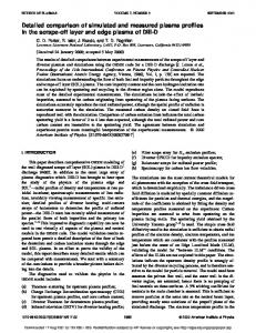
In CHS experiments, ECR-heating plasmas are characterized by peaked electron temperature and flat density profiles. Electron temperature can reach a few keV at the center in the low density regime (n e ⬃0.5⫻1013 cm⫺3), while ion temperature is low (⬃0.1 keV). The ECR-wave energy is directly transferred into the electron kinetic energy, then ions are indirectly heated up through collisions with hotter electrons. The difference in the operational condition of the lineaveraged density and the heating power P ECRH produces plasmas with electrons in different collisional regimes. The resulting potential profile alters according to the operational condition. The profile has been empirically classified into five representative patterns. Figure 3 shows the patterns in potential profiles of ECRheating plasmas with P ECRH⫽100 kW. The error bars in this figure represent standard deviation. Negative ␳ in Fig. 3 means that the observation point is located below the magnetic axis. The open and closed circles in Fig. 3 indicate the profiles termed bell and dome, respectively; the lineaveraged densities for bell and dome are ¯n e ⯝0.15⫻1013 cm⫺3 and ¯n e ⯝0.35⫻1013 cm⫺3, respectively. These profile patterns are observed in lower density or stronger ECRheating plasmas. In these two profiles a steep change in radial electric field, or a large E r -shear, can be seen at ␳ ⬃0.5 and ␳ ⬃0.25 for bell and dome, respectively. The open squares represent a rather simple profile, well expressed as a parabolic shape. This pattern is termed hill


4155

FIG. 3. Five typical shapes of potential profiles in ECR-heating plasmas. The ECR-heating power is fixed at 100 kW. The shapes are termed here 共a兲 bell, 共b兲 dome, 共c兲 hill, 共d兲 Mexican hat, and 共e兲 well. The potential shapes are changed according to the line-averaged density and the ECR-heating power.

profile here. The line-averaged density of this case is ¯n e ⯝0.5⫻1013 cm⫺3. The pattern shows no difference from those of bell and dome outside the position where a large E r -shear exists. The hill profile can be seen in the ECRheating plasmas in a density region where dome and bell patterns are observed. The hill pattern turns out, however, to be uniquely observed as the density becomes higher or heating power becomes weaker. As we describe later in detail, these three profiles are bifurcated states in low density regimes. In contrast to the above-mentioned profiles, the others are uniquely observed in a higher density regime. The closed squares show the Mexican hat profile, where the lineaveraged density is ¯n e ⯝0.8⫻1013cm⫺3. This profile is characterized by positive and negative electric fields around the core and periphery, respectively. The height of the hat decreases with an increase in the line-averaged density. As the density increases further and becomes closer to the density limit of ¯n e ⯝1.2⫻1013 cm⫺3, the potential profile gradually changes from Mexican hat shape into the so-called well shape. Changes in short length scale of ⬃1 cm are seen in the radial electric field of bell, dome, and Mexican hat profiles. There rather strong E r -shear exists in the core for bell and dome, and the periphery for Mexican hat profiles. These plasmas provide an interesting region for study, since the E r -shear could be associated with fluctuation reduction and resulting improved confinement modes. Actually, the formation of an internal transport barrier is confirmed for the plasma with the dome feature 共see Sec. VI兲. There, the relation between the fluctuation and the E r -shear is described with the formation mechanism of the transport barrier. Dependence of the profile patterns on the line-averaged density is more systematically described in Sec. VII.


4156


Fujisawa et al.

⫽0.6⫻1013 cm⫺3 and ¯n e ⫽1.5⫻1013 cm⫺3, respectively. Both potential profiles take on the well shape. Despite the two times difference in the density, the strength of radial electric field in the core region is similar. The same tendency has been already confirmed in the previous CXRS measurements in a wider density range.54 As the density increased, the radial electric field showed no significant difference in the core region of the NBI plasmas, while the radial electric field at the plasma edge became more negative. Consequently, the NBI plasma exhibits consistently a well shape of potential profile in a wide range of line-averaged density. In the ECR-heating plasma near the density limit, equipartition time between ion and electron becomes shorter. As a result, the ion temperature should have a value close to electron temperature near the density limit of ECR-heating plasmas. Then a thermal property similar to that of NBIheated plasmas is realized, and the potential profile of ECRheating plasma shows a well shape near the density. FIG. 4. Potential profiles in neutral beam injection 共NBI兲 heated plasmas. The open and closed circles show the potential profiles with the lineaveraged electron density of ¯n e ⫽0.6⫻1013 cm⫺3 and ¯n e ⫽1.5⫻1013 cm⫺3, respectively. Essentially, the potential profiles in the NBI-heated plasmas take the well shape without respect to the density. The increase in density makes the radial electric field at the periphery more negative, with keeping the radial electric field in the core region almost constant.

B. Patterns of potential profiles in NBI-heated plasmas

The NBI-heated plasma is characterized by a similar temperatures of electron and ion. Typically, both temperatures are about 0.2–0.3 keV in our experiments with field strength of 0.88 T, although high ion temperature modes have been reported in the low density plasma of ¯n e ⬃0.8 ⫻1013 cm⫺3 with field strength of 1.8 T.53 The high energy beam ions heat electrons more effectively than ions in our NBI-heated plasmas. The profiles of electron temperature, ion temperature and density are close to a parabolic shape. Figure 4 shows representative potential profiles in NBIheated plasmas with two different density cases. The open and closed circles represent the potential profiles for ¯n e

C. Potential profiles in ECR- and NBI-heated plasmas

Combined heating of ECR⫹NBI makes the plasmas regain the capability to exhibit all sorts of potential profile patterns in mere ECR-heating plasmas. The combined heating plasmas are characterized by high electron temperature (⬃1 keV兲 and lower ion temperature. The difference from the ECR-heating plasmas is a higher absolute value of ion temperature (⬃0.3 keV兲, since the injected neutral beam energy is directly transferred into ions with collisions. The electron collisionarity varies widely according to the lineaveraged density and the ECR-heating power. Potential profile patterns in the combined heating plasmas are considered to be essentially identical with those of ECR-heating plasmas. Two examples are presented to demonstrate the transient response of the potential due to switching the heating method and the potential profile in the combined heating phases. In the first example, ECR-heating of P ECRH⯝100 kW is applied on a target deuterium plasma sustained with NBI-heating. Figure 5共a兲 shows potential waveforms taken shot by shot for

FIG. 5. 共a兲 Time evolution of potentials at three radial points ( ␳ ⫽0, ␳ ⫽0.32 and ␳ ⫽0.48) when the ECR-heating is applied to the target plasma sustained with NBI. 共b兲 Potential profile in the steady state with a combined heating of ECR and NBI. The potential profile exhibits a similar feature to the bell shape in the ECR-heating plasma.




4157

FIG. 6. 共a兲 Time evolution of potential when the NBI-heating is applied to the target plasmas sustained with ECR-heating. 共b兲 Potential profiles in the later period of the combined heating phase of ECR and NBI. The potential profile has a characteristic of Mexican hat profile in the ECR-heating plasma. The dashed lines represent potential profiles in single ECR- or NBI-heating phases. A particular thing to note is that discontinuous changes in central potential are observed around t⫽55 msec.

several fixed spatial points. All potentials start to increase just after ECR-heating is applied. Only the central potential continues to increase after the other potentials at outer radii stop increasing 6 msec later. After 15 msec more, the plasma relaxes into a stationary state indicated by the arrow in Fig. 5共a兲. On the other hand, the line-averaged density begins to decrease after the ECR-heating is turned on, and reaches a constant value of ¯n e ⯝0.4⫻1013 cm⫺3 in the stationary state. Figure 5共b兲 shows the potential profile of the stationary state taken in the scanning mode in a sequential shot with an identical condition. The potential profile has a characteristic classified as the bell shape. After the ECR-heating is turned off, the potential profile starts to return to the potential profile with a well shape in 1–2 msec. In contrast to the previous, NBI-heating is placed over a deuterium plasma sustained with the ECR-heating of its maximum power P ECRH⬃300 kW. Figures 6共a兲 and 6共b兲 show the waveforms of the potential and its profiles in different heating phases, respectively. After the NBI application, the central potential increases by ⬃0.2 kV, keeping the

dome feature. Simultaneously, the potentials at outer radii of ␳ ⬎0.4 gradually change during the combined heating phase. Then the central potential monotonically decreases except for discontinuous changes around t⫽55 msec. This particular phenomenon will be discussed in the following subsection. The line-averaged density monotonically increases from ¯n e ⯝0.4⫻1013 cm⫺3 to ¯n e ⯝0.7⫻1013 cm⫺3 in this combined heating phase. The initial potential has the dome feature in the ECR-heating phase, as is shown by the dashed line in Fig. 6共b兲. In the later period indicated by the arrow in Fig. 6共a兲, the potential profile develops into a Mexican hat shape represented by the circles in Fig. 6共b兲. The height of the hat becomes lower gradually toward the end of the combined heating phase. After the ECR-heating is turned off, the potential profile starts to relax into a well shape in confinement time scale of 1–2 msec. These two examples demonstrate that the potential profiles show essentially identical characteristics with the ECR-heating plasmas.

FIG. 7. 共a兲 An expanded view of potential and detected beam intensity waveforms around t⫽55 ms in Fig. 6. Transition between discrete patterns of potential profiles. 共b兲 Expected potential profiles of two states that plasma makes the transition. The time scale of the change is in a few dozen microseconds at the fastest. This is much faster than the confinement time scale.


4158

Fujisawa et al.


FIG. 8. Self-sustained oscillation, referred to as electric pulsation, is observed in a combined ECR⫹NBI-heating phase. 共a兲 Pulsating behavior of the central potential of CHS plasmas 共solid line兲 in the lower density region. The dashed line represents the line-averaged electron density measured with a HCN interferometer. The line-averaged density in the stationary state is quite low at ¯n e ⯝0.4⫻1013 cm⫺3. 共b兲 Spatial structural change of the potential before and after transitions. Here ␳ is the normalized minor radius.

D. Transition between discrete patterns

The particular behavior to note is the discontinuous changes around t⫽55 msec in Fig. 6共b兲. Figure 7共a兲 shows an expanded view of the central potential for the events, together with the detected beam current intensity reflecting a local density change. The time scale of the changes is examined more accurately by fitting a function of tanh关(t⫺t0)/␶兴 to the slopes in the transient phase. The solid lines in Fig. 7共a兲 indicate the fitting curves. The obtained time constants for the abrupt drop and rise are ␶ ⫽60 ␮ sec and ␶ ⫽220 ␮ sec, respectively. The local density represented by the beam intensity should also change in similar time scale. The time scale is much faster than the energy confinement time of a few milliseconds. This is the first observation of transition in a radial electric field with a fine temporal resolution of microsecond order in toroidal plasmas. The spatial structure during the drastic change in the core potential is inferred from the measured potential changes at several spatial points. The open squares and closed circles are potential values before and after the transition, respectively 关see the arrows in Fig. 6共a兲兴. As is shown in Fig. 7共b兲, this dynamic behavior is localized in the core of ␳ ⬍0.4. These observations imply that the electric field of narrow region around ␳ ⯝0.25 changes from a positive to a negative value. The differences between potential signals from the three detectors of the HIBP also supports this expectation. This figure suggests, therefore, that the profile with the sharp peak turns into a flat or hollow profile. The hollowed potential profile has not been seen in the stationary state, therefore, this profile can exist only for a transient phase. Although it is difficult to obtain the fine structural change of profile during the transition happening in a few dozen microseconds, it is obvious that the plasma makes a transition between quite different and discrete patterns of potential profile. Therefore, this phenomenon shows that two different patterns of potential profile can be taken on the same bulk plasma parameters. This is definite evidence

for the bifurcation property in a potential profile or radial electric field in a toroidal helical plasma. IV. TEMPORAL PATTERNS IN POTENTIAL-VARIETY OF PULSATION A. Electric pulsation as stationary state

The bifurcation nature of the ECR-heating plasmas simply manifests itself as transitions between discrete patterns of potential profile. It is discovered, furthermore, that the bifurcation nature causes more drastic temporal patterns, a stationary self-excited oscillation in potential termed electric pulsation or potential pulsation. The phenomenon shows a number of variations and is considered to be repetitive back and forth transitions between bifurcated states. The most drastic patterns of electric pulsation are introduced as follows. The self-excited oscillations are maintained for a longperiod (⬃50 msec兲 after the ECR-heating is applied to the NBI-sustained plasma. The first example of electric pulsation is obtained in a hydrogen plasma to which almost maximum ECR-heating power ( P ECRH⬃300 kW兲 is applied. The solid and dashed lines in Fig. 8 show waveforms of central potential and line-averaged density, respectively. After the ECRheating is turned on, the central potential begins to increase and reaches its maximum with exhibiting pulses. The lineaveraged density decreases toward a stationary state of ¯n e ⯝0.4⫻1013 cm⫺3 in approximately 5 msec. In the stationary state from t⫽55 msec to t⫽95 msec, negative pulses of potential of ⫺0.6 kV quasi-periodically occur in approximately every 2 msec, or with frequency of ⬃0.5 kHz. The timescale of a pulse (⬃ a few dozen microseconds兲 is much faster than the diffusive one (⬃ a few milliseconds兲. Supposing that the oscillation is repetitive transitions between two distinct states, the potential profiles in the high and low potential states are roughly estimated from the time evolution of potentials at different radii 共details are discussed




4159

FIG. 9. Self-sustained oscillation, referred to as electric pulsation, is observed in a combined ECR⫹NBI-heating phase. 共a兲 Pulsating behavior of the central potential of CHS plasmas 共solid line兲 in the higher density region. The dashed line represents the line averaged electron density measured with a HCN interferometer. The line-averaged density in the stationary state is ¯n e ⯝0.7⫻1013 cm⫺3. 共b兲 Spatial structural change in potential before and after transitions.

in Sec. V B兲. Figure 8共b兲 shows the estimated potential profiles of two states. The profile in the high potential state has a bell shape as is seen in stationary states, while that in the low potential state has no identical one in stationary state. These data are taken with an identical operational condition shot by shot using the HIBP in the fixed-point observation mode. The profile in the low potential state is deduced by taking the statistical averages of local maxima or minima in periods including a pulse. Each data point of the high potential state is obtained by taking the statistical values between adjacent pulses. The time scale of the transitions is similar to that of the previous single pair of transitions observed in the deuterium plasma 共Figs. 6 and 7兲. However, in this example, the electric field around the core 共the first derivative of the potential兲 does not change considerably before and after the transitions. A large change of the electric field, as a result, occurs around the radial position of ␳ ⯝0.55 during a transition. In the present pattern, potentials at other locations also exhibit quasi-periodic pulses at similar intervals but with different amplitudes and polarities. In contrast to the pulses near the plasma center, positive pulses are observed in the outer plasma radii of ␳ ⯝0.55. The pulsation pattern alters with an increase in the lineaveraged density at the same ECR-heating power. Figure 9共a兲 shows the second example of pulsation seen in the central potential. After the ECR-heating application, the central potential increases and reaches its maximum of 0.3–0.4 kV. Simultaneously, the line-averaged density 共dashed line兲 decreases and relaxes to a steady state value of ¯n e ⯝0.7⫻1013 cm⫺3. During the combined heating phase of ECR⫹NBI, the line-averaged density increases gradually. Being accompanied with this slight increase, the amplitude and the frequency of pulsation become smaller and higher, respectively. The initial frequency of ⬃1.0 kHz increases to ⬃1.5 kHz in the later phase. Figure 9共b兲 shows the potential profiles before and after transitions in this case. Each point of data is taken in the period from t⫽50 msec to t⫽70 msec to avoid the characteristic change due to the bulk parameter difference. The plot

demonstrates that the potential profiles repeat transitions between two Mexican hat profiles with higher and lower domes during the pulsation, with the central potential change of about 0.3 kV. The profile change is limited inside ␳ ⫽0.6. The potential outside ␳ ⫽0.6 共x-marks兲 shows no change during the pulsation; the data of these locations are taken in the radial scan mode. The potential profile patterns between which plasmas repeat transitions are quite different from the first case of low density. The characteristics of electric pulsation vary according to the line-averaged density.

B. Flip-flop pattern

In the previous pulsations, the period of the low state is much shorter than that of the high potential state. The potential profile in the low potential state, hence, is allowed to be taken as a transient spatial pattern. Figures 10共a兲 and 10共b兲 present other pulsation patterns in the central potential. The solid and dashed lines in the figure represent the potential and the detected beam intensity, respectively. Both discharges were obtained in deuterium plasmas with only ECRheating whose power was 140 kW. The discharges have no NBI-heating. Consequently, the high energy ions of NBI are not an essential element to cause electric pulsation. The waveforms in the early phase of the discharges indicate a flip-flop behavior; the plasma alternately takes two discrete potential values in every ⬃1 msec. In the present patterns, both high and low potential states have an equivalent life time. The pulsation can be really regarded as the repetitive transitions between equilibrium states. The following measurements of potential profile with the identical condition confirm that the states with the low and high values correspond to the hill and dome states, respectively. Figure 10共a兲 shows that the central potential jumps up to a higher value in the later stage of the discharge. As is shown in Fig. 11, the profile of this new state has a bell shape. The beam intensity signals of the HIBP imply that the local densities should show no significant change in both discharges before the third branch appears. This result proves


4160

Fujisawa et al.


old to obtain the dome profile 共see Sec. VII兲. As the ECRheating power increases, the higher potential 共or bell兲 state becomes more stable, and the period of low potential state may become shorter. Then the pulsation patterns should be close to the previous two examples in which the full power of ECR-heating is applied. C. Other pulsation patterns

FIG. 10. Flip-flop patterns of electric pulsation in single ECR-heating plasma. The ECR-heating power is 140 kW. Two examples of time evolution of central potential 共solid line兲 and detected beam intensity 共dashed line兲 signals. 共a兲 The potential waveform shows transitions between three states A, B and C. 共b兲 The potential waveform shows transitions between two states A and B. In the early stage of both discharges, the behaviors are identical to each other. However, a transition to third state C occurs in the late stage of the discharge in the first case.

that there exist three bifurcation patterns 共bell, dome and hill兲 in the low density regime of ¯n e ⯝0.4⫻1013 cm⫺3. This observation suggests that potential structure should be remarkably sensitive to the bulk plasma parameters. The occurrence of a certain state could, as a result, be probabilistic. The ECR-heating power of 140 kW is close to the thresh-

FIG. 11. The potential profiles of three states in the flip-flop patterns of electric pulsation shown in Figs. 10共a兲 and 10共b兲. The potential profiles exhibit hill 共a兲, dome 共b兲 and bell 共c兲 features.

The difference in the line-averaged density and the ECRheating power brings about a variation of electric pulsation characteristics. Figure 12 shows two patterns observed in a combined ECR- and NBI-heating phase of hydrogen plasmas. In both discharges, the ECR-heating of 100 kW is applied to the NBI-target plasmas. The difference of these two discharges is the line-averaged density; 共A兲 ¯n e ⯝0.35⫻1012 cm⫺3 and 共B兲 ¯n e ⯝0.40⫻1012 cm⫺3. The solid and dashed lines in these figures represent the central potential and the detected beam intensity, respectively. The evolution of lineaveraged density and electron temperature measured with Thomson scattering is shown in Fig. 12共c兲. During the buildup of the potential, the central potential repeatedly shows small pulses with amplitude of ⬃0.1– 0.2 kV in both cases. The characteristics of each pulse have a similar feature to the previous electric pulsation or transitions. The phenomenon in Fig. 12 is a variation of electric pulsation. In a stationary state, both plasmas begin to exhibit regular pulses. The pulse amplitude becomes larger toward the end of the combined heating phase. In the low density discharge, the pulsation frequency obviously becomes lower as its amplitude increases. Furthermore, the correlation between the beam intensity signal and the potential pulse becomes clear. The electron temperature gradually increases after the ECR-heating is turned on. Each value of the temperature is the statistical average of similar discharges including the present examples. The electron temperature increase in the later phase of combined heating should be associated with the characteristic change of pulsation. The rapid changes of central potential signals at t⬃70 msec 共shot no. 76428兲 and t⬃76 msec 共shot no. 76436兲 suggest that the plasma should make a transition into the state characterized by higher potential or higher electron temperature. Figure 12共d兲 shows the ratio of the beam intensity from the plasma center to the line-averaged density. The ratio has a meaning of a peaking factor of density profile, since the change in the beam intensity should reflect a central density change in this low density region; the ratio should be pro¯ e . The signals imply that the density portional to n e (0)/n profile in the stationary states should have a similar shape, while the plasma in the single ECR-heating phase should have a more peaky density profile in the lower density discharge than that in higher density discharge. The difference in pulsation characteristics between these discharges is ascribed to the absolute value of density, which should be accompanied with temperature difference. A closer look at Fig. 12共b兲 gives us another finding that the amplitude of the pulses alternates two values of ⬃0.1 kV and ⬃0.05 kV. Figure 13 is an expanded view of the potential waveform from t⫽90 to 100 msec. In the pulsation pat-




4161

FIG. 13. Expanded view of the pattern of electric pulsation from t⫽90 ms to t⫽100 ms in the previous example 共shot no. 76436兲. The pulses with the half amplitudes are seen between pulses with regular amplitudes. It suggests the existence of an intermediate state.

tern of Fig. 8, similar small pulses with approximately half value are also seen between pulses with a regular amplitude. It could be interpreted that the potential in these two cases should make a transition from a high potential state to a certain intermediate state or fine structure. The behavior should give information of the detailed structure of bifurcation. D. Histograms as expression for pulsation characteristics

FIG. 12. Other pulsation patterns in a combined heating phase of ECR 共100 kW兲 and NBI 共800 kW兲. 共a兲 Central potential and detected beam intensity for the discharge whose density is ¯n e ⫽0.35⫻1013 cm⫺3. 共b兲 Central potential and detected beam intensity for the discharge whose density is ¯n e ⫽0.4⫻1013 cm⫺3. The detected beam intensity for the lower density discharge is presented by the gray dashed line for comparison. 共c兲 Time evolution of line-averaged density for two discharges. The statistical averaged electron temperature measured with Thomson scattering is represented by closed circles. The hatched area indicates the period when the transition should happen. 共d兲 Ratio of detected beam intensity to line-averaged density. The ratio has a meaning of a peaking factor.

The characteristics of pulsation patterns can be extracted by using a histogram expression of potential value appearing in the time evolution or waveforms. A histogram is made, for example, to clarify the characteristics of the flip-flop patterns in Figs. 10共a兲 and 10共b兲. Figure 14 presents the histogram expression of the flip-flop patterns of Fig. 10. In this histogram, the statistical frequency of potential value is normalized by the total number of ensemble. Therefore, the normalized histogram has a meaning of probability for realization of each potential value. Here, the waveform is digitized in every 20 ␮ sec and each data point is taken into the ensemble. The circles in Figs. 14共a兲 and 14共b兲 represent the normalized histogram or probabilities of central potential value of the central potential values. Three branches of the flip-flop pattern 关Fig. 10共a兲兴 are distinguished in the histogram as two prominent peaks around ␾ ⫽0.15 kV, ␾ ⫽0.9 kV and a diffusive band from ␾ ⫽0.3 kV to ␾ ⫽0.5 kV. The diffusive band corresponds to the potential profile with the dome feature. Two vague peaks are recognized in this band. It suggests that the dome branch may be composed of two fine structures. On the other hand, the spectrum of the flip-flop pattern with two states 关Fig. 10共b兲兴 shows a sharp peak at ␾ ⯝0.2 kV and a continuous band from ␾ ⫽0.3 to ␾ ⫽0.6 kV. The continuous band without any identical peak corresponds to the dome branch. The broadness of the band is caused by rather large fluctuations inherent with the dome state in this operational condition. Difference in the dome state property of these two discharges can be recognized in the histogram expression. The peak of


4162


FIG. 14. Normalized histograms of the flip-flop patterns. 共a兲 Probability of central potential values of the flip-flop discharge with three states 关see Fig. 10共a兲兴. 共b兲 Probability of central potential values of the flip-flop discharge with two states 关see Fig. 10共b兲兴. The dashed line represents the probability for the flip-flop patterns with three states as a reference.

the hill state in both discharges has a clear identity by their narrowness of full width at half-maximum 共FWHM兲. The histogram expression is applied to another ECRheating deuterium plasma showing three-state. Figure 15 shows the time evolution of the potential near the plasma center of ␳ ⯝0.21. Initially the plasma is stationary in the low potential state, then abruptly jumps to a higher potential state where irregular hesitating pulses, or rather large fluctuations are observed. Finally, the plasma develops into the oscillatory state showing a periodic pulsation. The beam intensity signal, which is represented by the dashed line, shows that a local density gradually decreases. Figure 15共b兲 is the histogram of the waveform of Fig. 15共a兲. It is recognized that there exist three identical states, which are indicated by the three peaks. The lower peak represents the hill branch, and the other two are expected to correspond to two dome branches appearing in the three-state flip-flop pattern; the dashed line shows the histogram of Fig. 14共a兲 for comparison. In the histogram indicated by the bold line, the second state showing turbulent nature (t⯝43 msec to t⯝50 msec兲 is expressed as a peak with a Gaussian-like fluctuation structure. The histogram expression or spectra of waveform gives a useful insight to identify bifurcated states, and clarify the characteristics of bifurcated states for their stability.

Fujisawa et al.

FIG. 15. Potential evolution exhibiting three states in an ECR-heating plasma. The ECR-heating power is 140 kW. 共a兲 Time evolution of the central potential 共solid line兲 and the detected beam current 共dashed line兲. The central potential develops from a quiet state to a state with large fluctuation through a transition. Then the potential makes another transition into a state with pulsation. 共b兲 The normalized histogram of potential values for this discharge. The dashed line represents the normalized histogram of the flip-flop discharge with three states 关see Fig. 10共a兲兴. Both histograms have similar peaks corresponding to hill and dome states.

V. DYNAMICS OF POTENTIAL STRUCTURE DURING PULSATION A. Behavior of plasma parameters during pulsation

Change of radial electric field causes or is caused by changes in bulk plasma parameters, such as temperature and density. Other diagnostic signals, in fact, are well correlated with the potential signal during electric pulsation. The pulsation pattern of Fig. 8, in which the correlation is the clearest, is chosen to demonstrate a close relationship between potential and thermal variables. Figure 16 shows signals correlated with the potential pulsation: 共a兲 potential signal as a reference, 共b兲 soft x-ray and electron cyclotron emission 共ECE兲, 共c兲 internal plasma pressure estimated from in-and-out asymmetrical evolution of Mirnov coil signals, and H ␣ signal, and 共d兲 line-averaged electron density. The soft x-ray emission along the central line of sight ( ␳ ⫹ ⫽0) decreases with the potential crashes, while the soft x-ray on an outer line of sight ( ␳ ⫹ ⫽0.4) increases 关Fig. 16共b兲兴. Here, ␳ ⫹ indicates the normalized smallest tangency radius of chordal measurements. This may be interpreted as a heat flux propagating from the inner to the outer region. An increase in the ECE 共93.5 GHz兲 signal from an outer region of the plasma ( ␳ ⬎0.5) supports this inter-




4163

FIG. 16. Correlation of the potential change with other plasma parameters during electric pulsation shown in Fig. 8. 共a兲 Potential signal at ␳ ⫽0.1 as a reference. 共b兲 Chord integrated soft x-ray emissions of two lines of sight of ␳ ⫹ ⫽0.4 and ␳ ⫹ ⫽0.0, together with ECE from the plasma edge region ( ␳ ⬎0.5). Here ␳ ⫹ indicates the normalized distance of a chord from the plasma center. 共c兲 Change of ⌬ ␤ estimated from plasma shift. The plasma shift is measured by Mirnov coils located at the inner and outer points on the equatorial plane, and H ␣ emission from the plasma edge. 共d兲 Line-averaged electron densities with ␳ ⫹ ⫽0.4 and ␳ ⫹ ⫽0.6.

pretation, although a plasma at such a low density is not sufficiently optically thick for the ECE to reflect the electron temperature. In the CHS magnetic configuration, the ECE has several resonant points, therefore, the change of the temperature profile cannot be deduced. Mirnov coils at the inner and outer points of the equatorial plane 关Fig. 16共c兲兴 indicate that the plasma starts moving inward, when the central potential reaches its minimum during a pulse. The internal energy measured by a diamagnetic loop and the average ␤ are about 400 J and 0.2%, respectively. The inward shift implies that the plasma loses an internal energy of about 20 J 共approximately ⌬ ␤ ⯝0.01%) with a potential pulse. This oscillation limits or deteriorates the confinement property of the plasma. The H ␣ emission also shows a good correlation with the potential pulses. The line-averaged density signals on chords of ␳ ⫹ ⬍0.4 show an increase synchronized with a potential crash, while the other ones on outer chords show no clear correlation; the lineaveraged density of ␳ ⫹ ⫽0.6 is given as an example in Fig. 16共d兲. In the present case of pulsation, its effect reaches plasma periphery, since the H ␣ signal is well correlated with pulsating potential. However, for the case of the electric pulsation with a higher base density, e.g., Fig. 9, the pulsation region becomes narrower around the plasma core. There, a correlation between these parameters and the potential pulse becomes less clear, and the effect is limited within a narrower region and the correlation with the H ␣ signal is ambiguous. B. Reconstruction of potential evolution during pulsation

The good correlation between a soft x-ray signal and the potential pulse makes it possible to reconstruct the spatio-

FIG. 17. The waveforms of potential during pulsation at 共a兲 ␳ ⫽0.0, 共b兲 ␳ ⫽0.21, 共c兲 ␳ ⫽0.43 and 共d兲 ␳ ⫽0.59. The bold lines represent statistical averaged waveforms, while the dashed lines show an example of the waveform without the average. The waveforms are obtained by taking the soft x-ray signal on the central chord as a reference clock. The bolder dashed lines are the standard deviation of each ensemble.

temporal evolution of the potential profile during pulsation by taking the central chord of a soft x-ray signal as a reference clock. In a discharge, more than a dozen pulses are available to produce their statistically averaged waveforms of potential. Here, the ensemble data is low-pass filtered with frequency of less than 10 kHz, and data points are taken with a sampling time of 10 ␮ sec. The time at which the soft x-ray crashes can be determined with a precision of ⬃10 ␮ sec. Figure 17 shows the potential waveforms for several radial points, 共a兲 ␳ ⫽0.0, 共b兲 ␳ ⫽0.21, 共c兲 ␳ ⫽0.43 and 共d兲 ␳ ⫽0.59. Solid and thin-dashed lines represent waveforms with and without statistical average, respectively. The point at t⫽0 means the beginning of the soft x-ray crash on the


4164


Fujisawa et al.

the next hundred microseconds until t⫽250 ␮ sec, the radial electric field at the periphery becomes positive, and the potential profile alters its shape a little slowly. The quasi-steady state profile at t⯝200 ␮ sec is shown by the open circles. After the plasma shows the profile indicated by the closed squares (t⯝250 ␮ sec兲, another transition occurs around the core at ␳ ⯝0.3. Then the plasma takes the intermediate potential profile with the dome feature, represented by the open squares, at t⯝300␮ sec. The potential profile rather gradually recovers to the initial state. In other words, the foot point of a strong shear of the radial electric field moves outwards. Approximately 2 msec later, almost the same process is repeated. C. Reconstruction of density profile evolution during pulsation

FIG. 18. Evolution of reconstructed potential profile during electric pulsation in Fig. 8. The potential profile in the high potential state at t⫽0 is represented by the closed circles. The potential profiles after the transition are shown at t⫽150 ␮ sec, t⫽200 ␮ sec, t⫽250 ␮ sec and t⫽300 ␮ sec.

central chord. The decrease in potential at ␳ ⫽0.0, ␳ ⫽0.21 and ␳ ⫽0.43 occurs at the same time as the soft x-ray crash within the present precision of a few dozen microseconds. At the location at ␳ ⫽0.0 and ␳ ⫽0.21, the time scale of the back transition from the low to the high potential state ( ␶ ⫽70– 90 ␮ sec兲 is of the same order as that of the forward transition ( ␶ ⫽25– 45 ␮ sec兲, where ␶ is the time constant of tanh关t/␶兴-fitting. At ␳ ⫽0.43, the potential gradually recovers into the high potential state after the forward transition of the same time scale as those at the above locations. For the waveform at ␳ ⫽0.59, the polarity of pulses is opposite to that of plasma inside. The potential rise has a delay of ⬃100 ␮ sec. The time scales of the potential rise and drop at this location are similar to those around core region. The bold dashed lines in Fig. 17 represent the standard deviation of each ensemble. The standard deviation has a minimum value at the time of the lowest potential value, and has a maximum in the slopes of fast potential change. The potential at each radial point should have a definite value that corresponds to the quasi-steady profile of the lower bifurcated state. The standard deviation should become smaller around the definite value. The time constants, however, are not exactly the same in each transition. This results in larger standard deviation on the process to reach the lower bifurcated state. The quasi-stable state, therefore, may be attained statistically at t⯝200 ␮ sec when the standard deviation reaches its minimum for all radial points. Using these waveforms, the evolution of potential profiles can be reconstructed during the pulsation. Figure 18 shows the evolution of the potential profiles during transitions. Closed circles represent the profile at the high potential state (t⫽0 ␮ sec兲, that is, the initial potential profile with the bell feature. The first transition happens in the radial electric field around ␳ ⯝0.5, and the potential profile changes into a shape represented by the open circles at t⫽150 ␮ sec. During

During the pulsation in Fig. 8, the detected beam intensity also exhibits a good correlation with the potential signal in a wide range of minor radius. The density of the discharges is sufficiently low for us to ascribe the change in the detected beam intensity to a local density change. Estimation of the attenuation factor ␣ in Eq. 共4兲 using the Lotz’s empirical formula55 gives a result that the condition of ␣ ⬍1 is actually satisfied in this low density plasma. Furthermore, the parameter ␣ does not make any significant difference for both completely flat and parabolic density profiles. Consequently, the change of the detected beam intensity ␦ I B (r) allows one to deduce a transient change of density profile during the pulsation except at the plasma edge.50 This correlation may give some insight into the causal relationship between the density and the radial electric field. Figure 19 shows time evolutions of the potential and the beam intensity signal for two different radii at ␳ ⫽0.43 and ␳ ⫽0.64. The increase 共or decrease兲 in the intensity at ␳ ⫽0.43 is correlated with a decrease 共or increase兲 in potential. The pulse polarity in the beam intensity at ␳ ⫽0.64 is opposite to that of ␳ ⫽0.43, although the correlation with potential pulses has the same property. The time constant of the beam intensity change is almost the same as that of the potential in the transition from the high potential state to the low potential state. Seemingly, the time constant of the beam intensity change, however, is faster than that of potential in the back transitions. In the discharges shown in Fig. 8, the line-averaged densities on several chords were taken shot by shot using the interferometer. The density profile can be reconstructed using the time-averaged value of each interferometer signal including pulses. The result obtained in this process should mainly reflect the density profile of the high potential state owing to its longer life time, although some small contribution in the low potential state is involved. Similar to the previous treatment of potential signals, statistical averages of the beam intensity signals during a pulse are obtained by taking the central chord of the soft x-ray as a reference clock. Assuming that the path integral effect is completely neglected, the ratio of beam intensity before and after transitions I B (t)/I B (t⫽0) are supposed to purely reflect the ratio of the local density change n e (t)/n e (t⫽0). Hence, evolution




4165

FIG. 19. Beam intensity signal of HIBP during electric pulsation in Fig. 8. Time evolutions of beam intensity signals at two different radial points, 共a兲 ␳ ⫽0.43 and 共b兲 ␳ ⫽0.64. The signals are well correlated with the pulsation in potential signals.

of the density profile during the pulsation can be inferred by multiplying the ratio to the Abel inverted density profile in the high potential state. Figure 20 shows 共a兲 the beam intensity signals of t ⫽0 ␮sec and t⫽300 ␮ sec as a function of normalized minor radius, 共b兲 the ratios of the beam intensity signals, and 共c兲 evolution of the reconstructed density profiles. The ratios and the reconstructed density profiles are presented at three points of time, t⫽150 ␮ sec, t⫽250 ␮ sec and t⫽300 ␮ sec. At the time of t⫽150 ␮ sec, a clear boundary of the change is seen at the location of ␳ ⬃0.4. The density increases inside the boundary, while it decreases outside. Then, the density profile recovers to the initial values of the high potential state after the density profile modification becomes localized around the boundary. The increase in density from t⫽0 ␮ sec to t⫽150 ␮ sec is from ¯n e (0)⯝0.4⫻1013 cm⫺3 to ¯n e (0)⯝0.7⫻1013 cm⫺3. The amount of change is quite large. In order to explain this increase in density, the necessary change of particle fluxes is approximately ␦ ⌫⬃3⫻1020 m⫺3 at ␳ ⬃0.4. The neoclassical fluxes accompanied with the absolute value of the radial electric field, however, is predicted to be only about ␦ ⌫ ⬃1019 m⫺3. Another mechanism should, therefore, play a role in the reformation of density profile. A possible candidate is convective fluxes induced by poloidal asymmetry in potential during the pulsation. Simultaneous measurements for poloidal asymmetry, using two beam probes, will have a great interest to clarify the structural reformation during pulsation.

FIG. 20. 共a兲 Profiles of the detected beam intensity after and before transitions. 共b兲 Profiles of ratios of beam intensity signals I B (t)/I B (0) at several times. 共c兲 Evolution of reconstructed density profile during electric pulsation using the detected beam intensity signals. The bold line indicates the density profile with Abel inversion in the high potential state. This suggests the density profile after transition from the high to the low potential state becomes a centrally peaked one.

VI. ELECTROSTATIC POTENTIAL AND THERMAL STRUCTURES A. Fine structure of the radial electric field

Many theories11–15 expect that a strong E r -shear or rotational shear affects plasma turbulence and suppresses the fluctuation driven transport. The electrode biasing experiments in the TEXTOR-94 have recently shown that fluctuation driven transport is reduced as the E r -shear increases.56 In the ECR-heating plasmas of CHS, a discontinuous change of the radial electric field in a narrow region, termed here a connection layer, is seen in the potential profiles with dome and bell features. In the connection layer, the E r -shear could


4166

Fujisawa et al.


shows the overall potential profiles of deuterium plasmas of interest. The potential profiles of the dome and hill are obtained with the ECR-heating power of 200 and 150 kW for the line-averaged densities of ¯n e ⫽0.4⫻1013 cm⫺3 and ¯n e ⫽0.3⫻1013 cm⫺3, respectively. Figure 21共b兲 shows the results of fine structural measurements in the profile with the dome feature. The fine structure was taken in an identical condition in the same day experiments with a spatial resolution of approximately 2 mm. Around the connection layer, the radial electric field is assumed to be expressed in a function form of tanh关(␳ ⫺␳0)/⌬c兴 since two different phases are considered to converge at ␳ 0 with a finite radial width of ⌬ c . The local potential profile around the connection layer is described as the integrated form of the function, that is,

␾ 共 ␳ 兲 ⫽A ln关 cosh关共 ␳ ⫺ ␳ 0 兲 /⌬ c兴兴 ⫹B ␳ ⫹C, where A, B, C are also the fitting parameters. By fitting the integrated function to the potential data in Fig. 21共b兲, the following results are obtained; A⫽0.028, ⌬ c ⫽0.047, ␳ 0 ⫽0.259 and B⫽⫺0.891. Figure 21共c兲 shows the obtained E r and its shear as a function of normalized minor radius. The E r -values inside and outside barrier are 7.8 ⫾0.7 kV/m and 1.7⫾0.3 kV/m, respectively. In real dimension, the FWHM of the E r -shear layer and the barrier position from the plasma center are 1.3⫾0.5 cm and 4.7⫾0.4 cm, respectively. The resulting E r -shear is ⬃39.7⫾17.4 V/cm2. As a reference, the potential profile of a simple hill shape is also shown in Fig. 21. Outside the connection layer, there is no difference between the potential profiles of the dome and hill. A simple parabolic function is well fitted to the hill profile, and the resulting shear is ⬃2 V/cm2. In the plasmas with the dome feature, the radial electric field inside ␳ ⯝0.25 is bifurcated into strongly positive branches from a weakly positive branch in which the radial electric field outside the radius still remains. B. Fluctuation around the connection layer

FIG. 21. Precise measurements around the barrier location using a HIBP. 共a兲 Potential profiles with different power of ECR-heating. The circles and the squares show the potential profiles with the power of 200 kW 共dome兲 and 150 kW 共hill兲, respectively. 共b兲 Fine structure of potential around the connection layer. Here two data sets from sequential shots are plotted. The dashed line represents potential profile of the hill state as a reference. 共c兲 Deduced E r -structure and its shear of the dome state. The dashed line shows the radial electric field of the hill state.

be sufficiently large to reduce the fluctuation. It is of a great importance to investigate the fluctuation and the transport around this regime. The potential profile with the dome feature can be easily sustained for a sufficiently long period in an operational condition. Elaborate experiments were performed to investigate the fine structure of the radial electric field around the connection layer in a potential profile with the dome feature, and to compare the fluctuation and thermal property between plasmas with the dome and the hill feature. Figure 21共a兲

The plasmas of the experiments are in a quite low density range of ¯n e ⯝0.5⫻1013 cm⫺3. Consequently, the fluctuation in the detected beam intensity ␦ I b (r) mainly reflects local fluctuation of density, except at the plasma edge.50 It is expected that the path integral term in Eq. 共4兲 should contribute to the fluctuation amplitude as a white noise. Density fluctuation around the shear-maximum point is measured shot by shot under the identical operation condition with the cases of Fig. 21. Figure 22共a兲 illustrates the fast Fourier transform 共FFT兲 spectra of fluctuation in the detected beam current from several spatial points for the dome state; ⌬r⫽0, ⫺3, ⫺1, ⫹1, and ⫹3 cm, where r represents the averaged minor radius. The point of ⌬r⫽r⫺r 0 ⫽0 cm is the nearest to the center position of the connection layer r 0 ⫽4.3⫾0.9 cm ( ␳ 0 ⫽0.23⫾0.05). The spectrum at ⌬r⫽0 cm shows a reduction in fluctuation power whose frequency ranges from 5 to 70 kHz, in comparison with other spectra at neighboring radial locations. In order to express the absolute power in a simple manner, Fig. 22共b兲 plots the integrated fluctuation power Q(⌬r)⫽ 兰 Pd f as a function of radius. The



FIG. 22. 共Color兲 Fluctuation in the dome state. 共a兲 Power spectra of density fluctuation at several radial positions around the shear-maximum radius. The red line represents the power spectra at the location of the shear maximum. 共b兲 Integrated fluctuation power as a function of the distance from the shear maximum radius ⌬r.

integral is performed from 5 to 70 kHz since the low frequency could contain other effects such as plasma movements. The power spectrum above 70 kHz just shows the nature of white noise, whose level is P base⬃1⫻10⫺5 . This fluctuation level could be mainly ascribed to the path integral effects, or the integrated fluctuation level on the beam orbit.50,52 The fluctuations independent along the beam orbit contribute to the base level of the fluctuation in the beam intensity. For comparison, Fig. 23共a兲 shows the power spectrum of the density fluctuation and its integrated power in the plasmas with a potential profile of the hill shape. In contrast to the previous spectrum, the power of the fluctuation monotonically increases toward the plasma edge. The power level is approximately twice larger than the dome state, as is shown in Fig. 23共b兲; thus, the absolute value of fluctuation is approximately ⬃ 冑2 times larger. The difference in the absolute fluctuation level could be ascribed to the lower density in this hill state. The peak frequency of this spectra shows no significant difference for all radii presented in this graph. Peak frequencies f p and the peak widths of these FFT spectra are estimated in the following manner. The peak frequency and its width are obtained by fitting the function of P( f )⫽ P 0 exp关⫺(f⫺f p) 2 /⌬ f 2 兴 ⫹ P base , to the spectrum around the peak, where P base , P 0 , f p and ⌬ f are the fitting parameters. These estimated values are shown in Fig. 24. Figure 24共a兲 shows that the peak frequency has a maximum, and that the normalized width ⌬ f / f p becomes narrower at


4167

FIG. 23. Fluctuation in the hill state. 共a兲 Power spectra of density fluctuation at several radial positions around the radius at which the dome profile shows the shear-maximum. 共b兲 Integrated fluctuation power as a function of the distance from the shear maximum radius ⌬r.

the shear-maximum point. Figure 24共b兲 also plots the peak frequency and its width in the plasma of the hill state. The figure shows the reduction in the fluctuation power at the shear-maximum point by 39%. This reduction rate is ¯ (1 cm)⫺Q(0) 兴 /Q ¯ (1 cm) with estimated from 关 Q ¯ (1 cm)⫽0.5关 Q(1 cm)⫹Q(⫺1 cm)]. The noise level of Q integral fluctuation can be assumed to be Q noise⯝70 ⫻10⫺5 . Then the reduction of fluctuation power at the shear-

FIG. 24. Peak f p and normalized width ⌬ f / f of frequency spectrum 共a兲 in the dome state, 共b兲 in the hill state. The circles and squares show the peak and normalized band width. The variable ⌬r represents the distance from the shear-maximum radius.


4168

Fujisawa et al.


FIG. 25. 共a兲 Electron temperature profiles for dome and hill states. 共b兲 Density profiles for the dome and hill states. The line averaged densities are ¯n e ⫽0.4⫻1013 cm⫺3 and ¯n e ⫽0.3⫻1013 cm⫺3 for the dome and hill states, respectively.

maximum point is 48% if the integral fluctuation level subtracted by the noise is used for the estimation. The radial electric field structure or its shear, therefore, has a large impact on the turbulence structure of the plasma. Furthermore, the reduced fluctuation should contribute to decreasing the fluctuation-induced transport. Hence a thermal transport barrier is expected at the connection layer. C. Transport at the connection layer

A Thomson scattering system was used to measure the profiles of electron temperature and density in the ECRheating plasmas indicating the hill and the dome feature in Fig. 25. The electron density of these two cases are not so high for obtaining sufficient photons to deduce local temperature and density in a single shot, therefore, approximately 20 shots are taken to obtain statistical averaged values of temperature and density. The results show clear difference in electron temperature profiles for these two states. The circles and squares in Fig. 25 represent the T e -profiles with the dome and hill states, respectively. The central temperature of the dome state is 2.0⫾0.2 keV, while that of the hill state is 1.4⫾0.1 keV. The T e -profiles outside the normalized radius of ␳ ⫽0.27 have no significant difference. The particular thing to note is that a

steep gradient change exists at the location of ␳ ⫽0.25 in the electron temperature for the plasma with the dome feature. The T e -gradients there are estimated as dT e /dr⫽⫺0.57 keV/cm and dT e /dr⫽⫺0.12 keV/cm for the dome and hill states, respectively. Figure 25共b兲 shows the n e -profiles measured with the Thomson scattering system. The n e -profiles have a flat or a slightly hollow shape for both cases. The line-averaged densities in the dome and hill states are ¯n e ⫽0.4⫻1013cm⫺3 and ¯n e ⫽0.3⫻1013cm⫺3, respectively. Around ␳ ⯝0.25 where the steep T e -gradient exists, no significant change can be seen in the density. The drastic change in pressure gradient exists at ␳ ⫽0.25 for the dome state. An energy transport barrier for electrons, consequently, is formed at the normalized radius of ␳ ⯝0.25. The experimental electron heat flux at the transport barrier is roughly estimated q exp⬃1⫻105 W/m2. According to a neoclassical theory,21,22 the electron heat flux there ( ␳ ⬃0.25) is estimated q neo⬃1 – 2⫻104 W/m2 in the hill state, when the available parameters of T e , n e and E r are taken into account. Hence, the anomalous transport should be dominant at that radius. On the other hand, the neoclassical electron heat flux can become closer to the level of the experimental value in the dome state owing to the higher temperature gradient. The estimation implies that the anomalous transport is reduced at the shear-maximum point. The location of the steep dT e /dr is in good agreement with the position of the E r -shear-maximum within the present error bar. It is suggested that the E r -shear reduction of fluctuation should, therefore, lessen the anomalous heat transport and form the transport barrier. Another peculiarity of the CHS transport barrier is that the density profile indicates no gradient change at the barrier location. This can be related to the importance of offdiagonal terms for the neoclassical particle flux in the toroidal helical plasma;21,22 e.g., Eq. 共1兲 is reduced into ⌫ Neo ⯝D TNeo⳵ T e / ⳵ r owing to the condition of ⳵ n e / ⳵ r⯝0. The neoclassical calculation gives the particle fluxes of ⌫ neo ⬃0.2⫻1020 m⫺2s⫺1 and ⌫ neo⬃1.5⫻1020 m⫺2s⫺1 at the barrier location for the hill and the dome states, respectively. In the dome state, a decrease in the fluctuation driven particle flux ⌫ fluc could compensate the neoclassical part enhanced by T e -gradient. D. E r -shear in other potential profiles

As has been already mentioned, a radial location of a significant E r -shear has been found in both Mexican hat and bell profiles. These profiles have a steep change in radial electric field at radii of ␳ ⯝0.5 and ␳ ⯝0.6. The strength of E r -shear is estimated for the region of these profiles to examine the possibility of the formation of internal transport barriers. Figure 26 shows fine structural measurements of the radial electric field around its shear maximum of the Mexican hat profile. The profile is taken in the plasma whose density is ¯n e ⯝0.8⫻1013 cm⫺3 with the ECR-heating power of 100 kW. The potential envelope around the shear maximum ( ␳ ⯝0.6) is shown in Fig. 26共a兲. It is less obvious in this case if



FIG. 26. A fine structural measurement of a potential profile with the Mexican hat feature. 共a兲 The potential profile around ␳ ⯝0.6, where the E r -shear has its maximum. 共b兲 The resulting radial electric field and its shear around the shear maximum.

two phases convergence is well assumed for the local shape of the potential. The results are obtained by fitting the integrated form of tanh关(␳⫺␳0)/⌬c兴 function to the envelope. The thickness of the connection layer is ⌬ c⫽0.11, which corresponds to ⬃2 cm in real dimension. The resulting shear is approximately ⬃6 V/cm2. The fitting process using a polynomial function gives a similar value as the estimated maximum shear. The value is expected to be too small to cause fluctuation reduction. The potential profiles with the bell feature are not stably sustained for a sufficiently long period. The profiles are usually linked with pulsation behavior in the experimental condition to date. The fluctuation has not been measured around that shear maximum point. Figure 27共a兲 shows the fine structure around the shear maximum ( ␳ ⯝0.5). The thickness of the connection layer is ⌬ c⫽0.052, which corresponds to ⬃1 cm. The resulting shear is approximately ⬃60 V/cm2, hence, the fluctuation reduction and the improved confinement are expected on the analogy of the potential profile with the dome feature. It is a matter for future work to find a region where the profile with the bell feature is stably maintained, and to investigate the temperature profile in the E r -shear maximum region. VII. EXPERIMENTAL BIFURCATION CHARACTERISTICS OF POTENTIAL A. Dependence of potential patterns on density

The presented observation of temporal and spatial patterns of the potential has demonstrated the bifurcation nature


4169

FIG. 27. A fine structural measurement of a potential profile with the bell feature. 共a兲 The potential profile around ␳ ⯝0.5, where the E r -shear has its maximum. 共b兲 The resulting radial electric field and its shear around the shear maximum.

of toroidal helical plasmas. The studies in these patterns show a close link between the thermal and the radial electric field structures. The bifurcation characteristics of the potential can be systematically understood by identifying the region in certain plasma parameters for each pattern to appear. So far, the line-averaged density has been treated as a representative parameter to indicate the plasma status with a given ECR-heating power, although the other plasma parameters are also changed with the line-averaged density. Electron temperature, for instance, decreases with an increase in the density. The bifurcation status of the plasma is considered to be expressed on a plane composed of the ECR-heating power and the line-averaged density. A series of experiments has been conducted for the purpose of making a map of potential profile patterns with a fixed heating power. The experiments were performed in hydrogen plasmas with ECR-heating in a wide range of line-averaged densities from ¯n e ⫽0.2⫻1013cm⫺3 to ¯n e ⫽1.2⫻1013cm⫺3. There the heating power was fixed at P ECRH⫽100 kW. Figure 28 shows the central potential values as a function of the lineaveraged density. Here 700–800 points of data are plotted in the diagram. The overall tendency is that the central potential decreases with an increase in the line-averaged density. Two critical values of the density are seen in this diagram, where the characteristics of the diagram change drastically. Below the first critical density of ¯n e ⯝0.5⫻1013 cm⫺3, higher potential values of ⬃0.4 kV can be obtained with a certain probability. As the density decreases further beyond the second critical value of ¯n e ⯝0.3⫻1013 cm⫺3, the potential value


4170


FIG. 28. Dependence of the central potential on the line-averaged density in the case of ECR-heating power of 100 kW. In low density regimes, bifurcations of the potential profile are observed at two critical values of density. Characteristic shapes of potential profiles are identical for five regimes.

up to ⬃1 kV can be reached. The bifurcation of potential profile patterns is considered to occur at these two critical values of the density. Five regions are identical on the diagram in correspondence with the five characteristic patterns of potential profile as already shown in Fig. 3. In the higher density region, the potential pattern is uniquely determined. In the region D from ¯n e ⬃0.6⫻1013 cm⫺3 to ¯n e ⬃1⫻1013 cm⫺3 along the low dashed line, the potential takes Mexican hat profiles. As the plasma becomes close to the density limit 共region E兲, the potential shows the well shape. Along the lower dashed line of ¯n e ⬎0.5⫻1013 cm⫺3, the profile gradually changes from the hill to the well through the Mexican hat shape. On the other hand, the plasma has a choice of three patterns in the potential profile in low density regime. In the region C along the low dashed line with the line-averaged density of ¯n e

Fujisawa et al.

⬍0.5– 0.6⫻1013 cm⫺3, the plasma can show a hill shape. Below the first critical density along the middle dashed line 共region B兲, the potential profile acquires the dome around the core, giving higher central potential. Below the second critical density along the high dashed line 共region A兲, the dome region expands to the outer radius of ␳ ⯝0.5, then the profile alters into the bell shape. Bifurcation diagrams of the radial electric field can be made for each radial position. The study shows that these two critical densities correspond to the bifurcation of the radial electric field at two different radii of the plasmas. Figure 29 shows the diagrams of the radial electric field at three radial positions of 共a兲 ␳ ⯝0.25, 共b兲 ␳ ⯝0.5 and 共c兲 ␳ ⯝0.75. The radial electric field is estimated by fitting a function to the measured potential. The radial electric field at ␳ ⯝0.25 is a unique function of the density above ¯n e ⬃0.5⫻1013 cm⫺3. However, a larger value of the radial electric field is allowed below this critical density, in other words, a bifurcation can take place at this density. Similar to this, the bifurcation of the radial electric field at ␳ ⯝0.5 occurs at the density of ¯n e ⬃0.3⫻1013 cm⫺3. In contrast, the radial electric field at ␳ ⬃0.75 decreases monotonically with an increase in the lineaveraged density. Hence no bifurcation on the density is identical in the periphery, although the change of radial electric field accompanied bifurcation could be less than the data scattering.

B. Hysteresis of bifurcation branch realization

It has been just shown in the previous bifurcation diagram that three branches of potential profile should exist in a low density regime of the ECR-heating plasma. The proposition is valid for plasmas with combined heating of NBI ⫹ECR. Bifurcation branches are able to be demonstrated by making a Lissajous diagram of the potential evolution as a function of the line-averaged density. The Lissajous diagram also reveals a hysteresis in potential on the density evolution. Examples are provided for this purpose in the following dis-

FIG. 29. Dependence of the radial electric field on the line-averaged density at three radial points. 共a兲 ␳ ⬃0.25. 共b兲 ␳ ⬃0.5. 共c兲 ␳ ⬃0.75. A density at which bifurcation occurs is found in the cases of ␳ ⬃0.25 and ␳ ⬃0.5. The radial electric field can bifurcate into a higher branch below the critical densities at ␳ ⬃0.25 and ␳ ⬃0.5. On the other hand, the radial electric field monotonically changes in the case of ␳ ⬃0.75.



FIG. 30. 共Color兲 Evolution of the potential and the line-averaged density in plasmas with a combined heating of ECR共100 kW兲⫹NBI共800 kW兲. 共a兲 The waveforms of the central potential and 共b兲 the line-averaged electron density. 共c兲 The Lissajous lines made of the central potential and the lineaveraged electron density. A clear hysteresis is seen; a clear difference in the density at which backward and forward transitions happen. Three distinctive branches exist for the combined phase of the ECR⫹NBI-heating, while the NBI phase has only one branch.

charges where the ECR-heating of P ECRH⬃100 kW and ⬃200 kW is applied to the target plasmas sustained with NBI-heating. Figure 30 shows three examples of time evolution of the central potential and the line-averaged density in deuterium plasmas. The plasmas in sequential shots have different initial densities that make their potential evolution quite different after the ECR-heating of 100 kW is launched. The initial densities of the plasmas are 共A兲 ¯n e ⫽0.2⫻1013 cm⫺3, 共B兲


4171

¯n e ⫽0.6⫻1013 cm⫺3, and 共C兲 ¯n e ⫽0.8⫻1013 cm⫺3. After the ECR-heating of P ECRH⬃100 kW is turned on, a rapid increase in potential and the following back-and-forth transitions, seemingly a pulse, are observed in the discharge with the lowest density 共case A; the green line兲. In the other two shots 共the red and blue lines兲, the potential gradually increases and transitions to upper potential states occur in the time scale of a few dozen microseconds. Then the potential gradually decreases. In the lowest density discharge 共case A兲, the line-averaged density monotonically increases after the launch of ECR-heating, while the other two shots show an increase in the density after an initial decrease. Bifurcation characteristics can be extracted from Lissajous traces of the potential and the density for sequential discharges with different initial densities. Figure 30 shows five Lissajous traces including the above three cases; the initial densities of the other discharges are ¯n e ⫽0.9⫻1013 cm⫺3 and ¯n e ⫽1.0⫻1013 cm⫺3. These Lissajous traces fall on curves to indicate four branches; three branches in the combined heating phase of ECR⫹NBI and one for the NBIheating phase. The three branches in the combined heating phase should correspond to those on the previous bifurcation diagram. Therefore, low, middle and high branches in Fig. 30 are termed here, for convenience, hill, dome and bell, respectively. Similar to the previous bifurcation diagram 共Fig. 28兲, two critical density values of ¯n e ⯝0.6⫻1013 cm⫺3 and ¯n e ⯝0.5⫻1013 cm⫺3 are identical, where the gradient of curves is altered. These critical values are different from the values of the previous diagram. This reason should be ascribed to the ion temperature difference owing to the NBIapplication. As for the Lissajous traces of case B 共the red line兲, the plasma status evolves as a loop of A-B-C-D-E-F during the combination heating phase. There are several transitions observed in a faster time scale than the confinement time scale. Initially after the launch of ECR-heating, the potential increases through point F along the hill branch. At point A, the plasma status becomes unstable, then transition occurs from the hill to the dome branch. Similarly, the transition from the dome branch to the bell branch occurs at point C. Then the plasma goes back to the dome branch in a confinement time scale, and potential gradually decreases along the line of the dome branch. Finally, back transition from the dome to the hill branch occurs at points E to F 关see Fig. 30共a兲兴. Clear hysteresis loops, therefore, exist for relationship between potential and density evolution. Also hysteresis and transition from the hill to the dome branch 共from point H to G兲 are seen in the Lissajous trace of case C 共the blue line兲. The second example is hydrogen discharges where higher ECR-heating power of P ECRH⬃200 kW is applied to NBI-sustained plasmas. The ECR-heating is launched with modulation in every 10 msec for a period of 10 msec. Figure 31 shows the time evolution of the potential and the lineaveraged density. As is similar to the other cases, the electron density starts to decrease, from ¯n e ⫽1⫻1013 cm⫺3 to 0.5⫻1013 cm⫺3, with a simultaneous increase in the potential after the ECR-heating is turned on. Then different behav-


4172


Fujisawa et al.

density is considered to be the bifurcation point from the dome to the bell branch. Below this density, another pulsation behavior between the bell and the hill branches occurs. As is similar to the diagram of Fig. 30, three bifurcation branches in the ECR-heating phase could be identified, although the low density part in the branches becomes unstable so that the pulsation behavior starts. Furthermore, an increase in the ECR-heating power should alter the path of potential evolution and should cause the pulsation. C. Probability of realization of potential profile patterns

FIG. 31. 共Color兲 Evolution of the potential and the line-averaged density with the power modulation of ECR-heating on NBI-sustained plasmas. The ECR-heating power of 200 kW repeats turning on and off alternately. Pulsation is seen below a critical density. 共a兲 Time evolution of the potential 共bold line兲 and the density 共dashed line兲. 共b兲 The Lissajous lines made of the potential and the density. Three branches can be identified on the traces of the ECR-heating phase.

ior from the previous case appears clearly. The plasma begins to exhibit potential pulsation with negative pulses at the center above a critical potential or below a critical density. After the ECR-heating is turned off, the potential decreases and the electron density starts to recover. At the same time, the electric pulsation terminates. Lissajous traces are made of these waveforms of the potential and the line-averaged density. Several Lissajous traces with different densities of target NBI-heated plasma are shown in the diagram. The envelope along the plasma evolution draws outlines of bifurcation branches. There can be seen three critical points in this diagram. A steep change in the gradient of ⳵ ␾ / ⳵ n e is observed at the critical density of ¯n e ⯝0.6⫻1013 cm⫺3. After ECR-heating launch, the plasma evolves directly from the hill to the dome branch at this first bifurcation point, while the previous plasma with P ECRH⬃100 kW passes through the first bifurcation point to the hill branch. Below the critical density of ¯n e ⯝0.5⫻1013 cm⫺3, the pulsation between dome and hill branches begins to occur with an increase in its amplitude and a decrease in density. Another steep change in the gradient can be recognized at the critical density of ¯n e ⯝0.45⫻1013 cm⫺3. This

The existence of several bifurcation branches or multiple states makes it uncertain which potential profile is actually realized even if the line-averaged density and the ECRheating power are given with an identical operational condition. In the previous subsection, hysteresis of the evolution of the potential profile is actually observed, and two or three states are realized at a density with the same ECR-heating power. A probabilistic treatment, therefore, is possible for realization of three branches of potential structures of ECRheating plasmas in lower density regime. The probabilistic treatment is, for instance, performed on the data set shown in the bifurcation diagram of Fig. 29. Normalized histograms or probability distribution functions of the radial electric field at ␳ ⯝0.25 and ␳ ⯝0.5 are ¯ e ⬍0.6⫻1013 made for five density ranges, 共A兲 0.5⫻1013⬍n ¯ e ⬍0.5⫻1013 cm⫺3, 共C兲 0.2⫻1013 cm⫺3, 共B兲 0.3⫻1013⬍n 13 ⫺3 ¯ ⬍n e ⬍0.3⫻10 cm and 共D兲 ¯n e ⬍0.2⫻1013 cm⫺3. The probability distribution functions are obtained by normalizing the number of data taking an E r -value by the total number of ensembles and step widths of the radial electric field ⌬E r chosen as 0.5 kV/m. Figure 32 shows the probability distribution functions at ␳ ⯝0.25 共open circles兲 and ␳ ⯝0.5 共closed circles兲. In range A of the highest density, the functions at ␳ ⯝0.25 and ␳ ⯝0.5 have clear sharp peaks at E r ⯝0.5 kV/m and E r ⯝1.0 kV/m, respectively. The FWHM of the peaks are ⌬E r ⫽0.37 kV/m and ⌬E r ⫽0.33 kV/m at ␳ ⯝0.25 and ␳ ⯝0.5, respectively. Usually only the hill branch is realized in this density range. The sharpness of these peaks also indicates that the hill branch is quite stable. As the density decreases to range B, a small broad peak appears at E r ⯝5.2 kV/m in the distribution function at ␳ ⯝0.25. The FWHMs of sharp and broad peaks are ⌬E r ⫽0.58 kV/m and ⌬E r ⫽1.36 kV/m, respectively. On the other hand, the distribution function at ␳ ⯝0.5 has a sharp peak at E r ⯝1 kV/m with its FWHM of ⌬E r ⫽0.36 kV/m. This result indicates, therefore, that the dome branch begins to appear in this density range. However, the broadness of the dome branch peak indicates that the state should not be so stable, or that the radial electric field at ␳ ⯝0.25 E r (0.25) should have a rather large fluctuation. Further density decrease makes both sharp peaks at ␳ ⯝0.25 and ␳ ⯝0.5 become diffusive, and form continuous bands up to more than E r ⫽10 kV/m. In range C, the peak at ␳ ⯝0.25 around E r ⯝1 kV/m is strongly distorted from a Gaussian-like shape. In the distribution function at ␳ ⯝0.25




4173

FIG. 33. The radial electric field at ␳ ⫽0.25 as a function of the radial electric field at ␳ ⫽0.5 in a density range of ¯n e ⫽0.5⫻1013 cm⫺3 for the ECR-heating power of 100 kW.

band up to E r ⬃10 kV/m begins to be formed in the probability distribution function at ␳ ⯝0.5. The broadness of the band indicates that the bell branch is not stable. It was actually observed in the experiments that the bell branch had a shorter life time for this low ECR-heating power of 100 kW. In ranges C or D, both bell and dome branches can be realized with a finite probability. Figure 33 shows at the E r (0.5)-value as a function of E r (0.25) for the density range of ¯n e ⬍0.5⫻1013 cm⫺3. The dense region in the figure is where the profiles of hill and dome are realized. The scattering points, which have a much smaller population, on the upper-right side mean the appearance of the bell profile. A simple estimate shows that the realization probabilities for dome and bell are approximately 20% and 5% in the density range of ¯n e ⬍0.5⫻1013 cm⫺3 for rather low power P ECRH ⯝100 kW. D. Dependence of patterns on ECR-heating power FIG. 32. Normalized histograms of the radial electric field values for the data of Fig. 24. The normalized histograms are made for four density ranges, ¯ e ⬍0.6⫻1013 cm⫺3, 共b兲 0.3⫻1013⬍n ¯ e ⬍0.5⫻1013 cm⫺3, 共c兲共a兲 0.5⫻1013⬍n 13 ¯ 13 ⫺3 ¯ 0.2⫻10 ⬍n e ⬍0.3⫻10 cm and 共d兲 n e ⬍0.2⫻1013 cm⫺3. The solid 共open兲 and dashed 共closed兲 lines 共circles兲 represent the normalized histograms at ␳ ⯝0.25 and ␳ ⯝0.5, respectively. The realization probability of the potential profile with the dome or the bell feature is much lower than that of the hill shape in the case of P ECRH⯝100 kW.

in the density range, two peaks are found in the region of E r ⬎3 kV/m. This suggests that two fine structures may exist for the dome branch in the lower density regime, as was suggested in flip-flop pattern discharge 关see Figs. 10共a兲 and 14共a兲兴. On the other hand, the sharp peak at ␳ ⯝0.5 still keeps a Gaussian-like shape with the FWHM of ⌬E r ⫽0.52 kV/m. Finally, in range D, of the lowest density, a continuous

As the heating power increases, the probability for plasmas to take higher potential branches 共dome or bell兲 is expected to increase. Figure 34 shows dependence of the potential profile patterns on the ECR-heating power in hydrogen plasmas. The potential profiles were obtained in sequential shots. The line-averaged density in the experiment is kept constant of ¯n e ⯝0.4⫻1013 cm⫺3. With the ECRheating power of 130 kW, the potential profile 共squares兲 just shows the hill feature. As ECR-heating power increases up to 150 kW 共open circles兲, the profile abruptly changes to acquire the dome feature. The feature is lost again by further increase in the ECR-heating power up to 190 kW, then the potential profile shows the bell feature. The profile with the dome feature is obtained in a certain window of the ECRheating power for a fixed density. The threshold power for the dome feature has been empirically estimated as P ECRH⯝150 kW for the line-averaged


4174

Fujisawa et al.


FIG. 35. Dependence of the pulsation characteristics on the line-averaged electron density. 共a兲 The pulsation frequency observed in the central potential versus the line-averaged density. 共b兲 The pulsation amplitude of the central potential versus the line-averaged density. Here, the port-through NBI- and ECR-heating powers are 700 and 300 kW, respectively. FIG. 34. Dependence of the potential profile on the ECR-heating power. The square, open circles, closed circles and x-marks represent the potential profiles with ECR-heating power of 130, 150, 170, and 190 kW, respectively. The line-averaged density here is fixed at n e ⯝0.4⫻1013 cm⫺3.

density of ¯n e ⫽0.4⫻1013 cm⫺3. In this operational condition, the probability for realization of the dome feature will indicate a sharp peak in the normalized histogram. Then, the separation of peaks between the dome and the hill branches could become clearer, compared with the case of P ECRH ⬃100 kW. The probability for the dome branch will become higher with an increase in the ECR-heating power until the probability for the bell feature becomes dominant. The concepts of the power threshold and the critical density can be exactly defined in a strict sense after the probabilistic base is formulated. Some other branches, such as oscillatory steady states, turn to occupy a certain amount of regime on the bifurcation diagram as the ECR-heating power increases. Pulsating behavior, or a stationary oscillatory state, should be also expressed in a bifurcation diagram, as well as steady potential patterns. Under the fixed ECR-heating power of P ECRH ⯝100 kW, the pulsating behavior in potential is seen in some discharges in the extremely low density region of ¯n e ⯝0.2 ⫻1013 cm⫺3. This case suggests that the threshold for pulsation may be P ECRH⬃100 kW for the density of ¯n e ⯝0.2 ⫻1013 cm⫺3. The following estimate of the power threshold is given in other experiments: P ECRH⬃200 kW for ¯n e ⯝0.5 ⫻1013 cm⫺3, and P ECRH⬃300 kW for ¯n e ⯝0.7⫻1013 cm⫺3. It is preliminarily expected that pulsation threshold should be apparently proportional to the density. Furthermore, the pulsation characteristics such as the pulsation frequency, the pulse amplitude, and the bifurcated states that the plasmas make transitions to, alter according to the line-averaged density and the ECR-heating power. The pulsation patterns presented in the previous section would be mapped onto a certain regime on the ECR-heating power and the line-averaged density. Dependence of the pulsation frequency and the amplitude on the line-averaged density is

preliminarily obtained at a fixed heating power. Figure 35 presents the dependencies obtained in the combined heating phase of NBI⫹ECR, where ECR-heating power is nearly at its maximum of ⬃300 kW. There, it is obvious that the pulsation amplitude becomes smaller and the pulsation frequency becomes higher as the density increases. It is a future work to make a complete bifurcation diagram including power dependence. VIII. COMPARISON WITH NEOCLASSICAL THEORETICAL EXPECTATION A. Bifurcation characteristics in neoclassical theory

The bifurcation property of the radial electric field in toroidal helical plasmas has been predicted with neoclassical theories including helical ripple effects. In a neoclassical frame work, a local balance of radial fluxes of electrons and ions determines the radial electric field if the bulk plasma parameters are given, such as density, temperature, their gradients, and amounts of impurities. Equation 共3兲 allows us to draw a neoclassical bifurcation diagram for a radial position as a function of the electron temperature and density. Figure 36 is an example of a neoclassical bifurcation diagram made by use of the Hastings formula.22 The necessary parameters are assumed to be in a plausible range of the CHS experimental values; B⫽0.9 T, T i ( ␳ )⫽0.3 keV, Z eff ⫽2, ⳵ ln ne(␳)/⳵␳⫽0 and ⳵ ln Te(␳)/⳵␳⫽⳵ ln Ti(␳)/⳵␳⫽⫺1.1. The ion species is assumed to be hydrogen. The helical ripple and toroidal coefficients 共or inverse aspect ratio兲 are chosen as ⑀ H⫽0.063 and ⑀ T ⫽0.16, respectively, corresponding to ␳ ⯝0.5 of the CHS plasma. The temperature gradients also correspond to that at ␳ ⫽0.5 in a parabolic form. The bold and thin dashed lines in Fig. 36 represent the contours of the radial electric field for E r ⫽0 and the other values, respectively. The crescent region represents an area where multiple solutions exist inside. Two examples of the radial electric field along a line crossing the crescent region are shown in Figs. 36共b兲 and 36共c兲. Figure 36共b兲 shows the radial electric field as a function of the electron density with




4175

FIG. 37. 共a兲 Difference of the radial electric field between two branches, E gap . 共b兲 The maximum value of neoclassical radial current during transition j max . The values are calculated along the boundaries of the crescent regime in Fig. 36共a兲. Here, H and L means the branches of high and low radial electric fields, respectively.

the bifurcation point, a slight deviation from an equilibrium radial electric field induces radial current flowing in the direction to enhance the change of the radial electric field. During the transition, the radial electric field evolves obeying the following equation:1,7

⑀⬜ ⑀ 0

FIG. 36. A neoclassical bifurcation diagram. The assumptions used in the calculation are T i ( ␳ )⫽300 eV, Z eff⫽2, ⳵ ln ne(␳)/⳵␳⫽0 and ⳵ ln Te(␳)/⳵␳ ⫽⳵ ln Ti(␳)/⳵␳⫽⫺1.1. We choose ⑀ h ⫽0.063 and ⑀ t ⫽0.16, which corresponds to ␳ ⯝0.5 of the CHS hydrogen plasma. 共a兲 Radial electric field as a function of electron temperature and density. Multiple steady states exist in the hatched region on the n e ⫺T e plane 共shaded region兲. Contours of the constant electric field are shown by dashed lines. 共b兲 Bifurcation curve of the radial electric field as a function of density. A constant electron temperature is assumed; T e ( ␳ )⫽0.5 keV. 共c兲 Bifurcation curve of the radial electric field as a function of temperature. A constant density is assumed; n e ( ␳ )⫽5⫻1012 cm⫺3.

a fixed temperature of T e ⫽0.5 keV, while Fig. 36共c兲 does that as a function of electron temperature with a fixed density of n e ⫽0.5⫻1013 cm⫺3. Both curves show three branches of solutions. An unstable solution 共dashed line兲 exists between two stable ones 共solid lines兲. In other words, the unstable branch forms a forbidden band between the radial electric field actually realized. The curves indicate a subcritical bifurcation nature. This characteristics allow a hysteresis of radial electric field on the evolution of bulk plasma parameters, as well as a drastic change of radial electric field in time and space. B. Transition in neoclassical theory

Transition occurs between two stable solutions if the plasma satisfies a condition on the crescent boundaries. At

⳵Er ⫽⫺ j r 共 E r 兲 . ⳵t

共5兲

Here, ⑀⬜ ⫽M tor(1⫹c 2 / v A2 ) with M tor⯝1⫹2q 2 is the perpendicular dielectric coefficient of plasma, where q, v A and c are the safety factor, Alfve´n and light velocities, respectively. The factor M tor is termed the toroidal enhancement factor. The time scale of the transition is determined by the magnitude of the radial current and dielectric constant. The neoclassical radial current during a transition is approximately expressed by a simple form as j r (E r ) 2 , where j max , E H and E L ⬃4 j max(E r ⫺E H )(E r ⫺E L )/⌬E gap are the maximum radial current during the transition, and the values of radial electric field of high and low branches, respectively, and ⌬E gap(⫽E H ⫺E L ) represents the gap of the radial electric field between two stable branches. Assuming the parabolic form of radial current, the solution can be expressed as a simple form of tanh关(t⫺t0)/␶Neo兴 , with the time constant of ␶ Neo⯝ ⑀⬜⑀ 0 ⌬E gap/2j max . For instance, two quantities to estimate the transition time constant, ⌬E gap and j max , are plotted in Fig. 37 as a function of the electron density along the boundaries of the crescent regime in Fig. 36共a兲. C. Comparison with experimental results

The neoclassical bifurcation property of the radial electric field could be associated with the cause of electric pulsation and formation of transport barrier. In the neoclassical theoretical frame, electric pulsation can be a stationary state where repetitive transitions take place between two stable branches in the radial electric field. The internal transport barrier is formed after the radial electric field inside the connection layer bifurcates into a strongly positive branch with the radial electric field outside remaining in the weakly positive branch. The formation of the connection layer and the


4176


FIG. 38. A comparison between neoclassical and experimental E r in a NBIheated plasma. 共a兲 Profiles of ion, electron temperatures, and electron density. 共b兲 The experimental profile of the radial electric field, and the radial electric field predicted by the neoclassical theory using the above plasma parameters.

electric pulsation could, therefore, be the manifestation of neoclassical bifurcation nature of radial electric field in space and time, respectively. The plasma parameters in these two phenomena are in a range 共a crescent regime兲 possible for occurrence of the neoclassical bifurcation within the present experimental precision. Detailed comparison can be made between neoclassical and experimental radial electric fields in a few cases of NBIplasmas. Almost all parameters are available to predict the radial electric field with the neoclassical theory; there the ion temperature profile is known from the CXRS experiments. Figure 38 shows an example of the comparison between theory and experiment. The profiles of bulk plasma parameters, such as ion temperature, electron temperature and density, are also shown in Fig. 38共a兲. It can be said for this case that a good agreement is achieved, although the theoretical expectation gives an absolutely lower value than that of experiments. The neoclassical theory also gives a qualitative explanation of the positive electric field observed in the ECR-heating plasmas where the electron temperature becomes higher than the ion temperature. Another comparison between experiments and neoclassical theories can be made in transition time scales. A number of transition time scales are evaluated in electric pulsation. Figure 39 shows typical waveforms of backward 共low

Fujisawa et al.

FIG. 39. Examples of waveforms of the central potential during the transition. 共a兲 Experimental time scale of the transitions observed in the electric pulsation in Fig. 8 共low density case兲. 共b兲 Experimental time scale of transitions observed in the electric pulsation in Fig. 9 共high density case兲.

to high potential state兲 and forward 共high to low potential state兲 transitions near the plasma center from the previous two cases, 共a兲 a pair of typical transitions in low density pulsation of Fig. 8, and 共b兲 that in higher density of Fig. 9. The characteristic time constants of transitions can be well estimated by fitting the tanh关t/␶兴 function to the slope during transitions. The typical time constants are a few dozen and near 100 ␮s for forward and backward transitions, respectively. It is an experimental feature that the forward transition is faster than the backward one. Figure 40 shows a result of the comparison in transition time constants 共a兲 for the forward and 共b兲 the backward transitions. The closed circles represent the averages of the experimental constants in the plasma core for three values of the line-averaged density. The error bars indicate the standard deviation of the ensembles that consist of more than a dozen transitions. The solid lines represent the neoclassical constants with the following plasma parameters; B⫽0.9 T, Z eff⫽2, ⑀ t ⫽0.16, ⳵ ln ne(␳)/⳵␳⫽0, ⳵ ln Ti(␳)/⳵␳⫽⫺1.1, T i ( ␳ )⫽0.3 keV, ⳵ ln Te(␳)/⳵␳⫽⫺1.1, and ⑀ h ⫽0.063. In order to consider the uncertainty of the measured parameters, the hatched region indicates the range of the time constant when a parameter varies with others being the same. The ranges of parameter change are T i ( ␳ )⫽0.3– 0.4 keV, ⳵ ln Te(␳)/⳵␳⫽⫺3 to ⫺1.1, and ⑀ h ⫽0.063– 0.092. Both experimental and theoretical time constants have



FIG. 40. Comparison between the neoclassical and the experimental time constants of the transition at several density values. 共a兲 Time constant for the forward transition. 共b兲 Time constant for the backward transition. The closed circles represent the experimental values. The solid line indicates the theoretical values when the plasma parameters are assumed to be those of Fig. 5. The other lines are the theoretical values with different assumptions of the plasma parameters as follows. 共I兲 T i ( ␳ )⫽0.3 keV, ⳵ ln Te(␳)/⳵␳⫽⫺1.1, ⑀ h ⫽0.063. 共II兲 T i ( ␳ )⫽0.4 keV, ⳵ ln Te(␳)/⳵␳⫽⫺1.1, ⑀ h ⫽0.063. 共III兲 T i ( ␳ ) ⫽0.3 keV, ⳵ ln Te(␳)/⳵␳⫽⫺3, ⑀ h ⫽0.063. 共IV兲 T i ( ␳ )⫽0.3 keV, ⳵ ln Te(␳)/⳵␳⫽⫺1.9, ⑀ h ⫽0.092. 共V兲 T i ( ␳ )⫽0.4 keV, ⳵ ln Te(␳)/⳵␳⫽⫺1.9, ⑀ h ⫽0.092. The case 共I兲 has the same parameters as those of Fig. 36. In cases 共IV兲 and 共V兲, the helical ripple coefficient corresponds to the value of ␳ ⫽0.6, and the electron temperature gradient is also the value of a parabolic profile at ␳ ⯝0.6.

an agreement in the tendency that the backward transition is slower than the forward one. The experimental time constants are in the range of the theoretical expectation within the present precision of the experiments. The transition time constant is, therefore, expectable with the neoclassical calculation for the plasma core region. In other words, the neoclassical unbalanced particle flux could be a main contribution to the radial current to proceed the transition. D. Nonlinear relationship between the radial current and radial electric field

Further detailed comparison between the experiment and the theory is possible in behavior during transition, how the radial current is dependent on the radial electric field. Equation 共5兲 allows one to deduce the experimental radial current during the transition. The temporal resolution of HIBP is


4177

FIG. 41. 共a兲 The experimental radial current to induce the radial electric field change. The solid and the dashed lines show the radial current and the radial electric field, respectively. 共b兲 The experimental radial current j r as a function of the radial electric field E r . The open circles are plotted in every 64 ␮ sec. 共c兲 Neoclassical relationship between the radial electric field and the radial current at bifurcation points. In this calculation, the plausible plasma parameters are assumed for the experimental condition for the above transitions to occur.

sufficient to evaluate the time derivative of the radial electric field. Using a wavelet analysis on the estimated average electric field, the radial current during the transition is evaluated for the case of Fig. 7. Figure 41共a兲 shows the radial current, where the perpendicular dielectric constant is ⑀⬜ ⯝2.7⫻104 for q⯝3 and the Alfve´n velocity v A ⯝8⫻106 m/sec, which corresponds to the electron density ¯n e ⫽0.3⫻1013 cm⫺3. In the estimate, the averaged field given by ¯E r ⫽⫺ 关 ␾ (0.3a) ⫺ ␾ (0) 兴 /0.3a is used instead of the local radial electric field. The maximum currents are 4.5⫾3.0 A/m2 and ⫺3.6 ⫾2.4 A/m2 for the forward (t⫽54.6 msec兲 and backward (t⫽56.0 msec兲 transitions, respectively. The error bars in the


4178


electric field and radial currents come from the uncertainty of the potential change at ␳ ⫽0.3. Figure 41共b兲 plots the radial current as a function of the radial electric field 共E-J curve兲 using the wavelet analysis. The dashed line represents the E-J curve obtained using the tanh-fitting to the change of radial electric field. The difference between two cases represents the uncertainty due to the evaluation method. These curves demonstrate the nonlinear dependence of the radial current on the radial electric field to make the transitions occur. Figure 41共c兲 indicates two examples of the neoclassical radial current during the transitions as a function of the radial electric field.21,22,40 In this calculation, plausible parameters of the CHS plasma are chosen to satisfy bifurcation conditions. The profiles of ion temperature and electron density in calculation are assumed to be all parabolic, with the central values being 0.35 keV and 0.5⫻1013 cm⫺3. The central electron temperatures are assumed to be 0.63 and 0.8 keV for cases 共I兲 and 共II兲. The neoclassical radial current ⬃5 A/m2 is within the range of the experimental value. The topology of the E-J curve is identical to the experimental one. The neoclassical theory can, therefore, give an essential description to the transition or bifurcation property of toroidal helical plasmas. IX. DISCUSSION A. Effect of high energy particles on pattern formation in potential

High energy particles may play a role in the formation of potential and oscillatory stationary states. Loss cone loss particles produce electric current to contribute to the formation of potential. The equation giving solutions of the radial electric field needs correction due to the loss cone loss current in LC Neo the following form, ⌫ Neo i (E r )⫹⌫ i (E r )⫽⌫ e (E r ) LC LC LC ⫹⌫ e (E r ), where ⌫ i and ⌫ e represent ion and electron loss cone currents, respectively. The previous theoretical work shows that the ion loss cone current does not make any significant difference in the radial electric field in the CHS case.40 On the other hand, it was experimentally observed that a transition was forced to occur when ECR-heating of 140 kW was applied at the plasma periphery.24 The result was explained by electron loss cone current enhanced by the ECR-heating. A number of results from plasmas associated with onaxis resonance ECR-heating have been presented in this article. It is worthwhile, therefore, discussing the electron loss cone and its effect on the formation of potential. A peculiarity to be mentioned for toroidal helical plasmas is that loss cone structure is tightly associated with the potential structure. An analytical formula can be used to evaluate loss cone boundaries for electrons and ions.38 Figure 42 illustrates two cases of loss cone structure for deeply trapped electrons for the plasmas whose central potentials are 1.0 and ⫺0.3 kV, with its profile assumed to be parabolic. Values of ⑀ T (a) ⫽0.16 and ⑀ H (a)⫽0.255 have been assumed for the CHS configuration. In the case of positive potential 关 ␾ (0)⫽1.0 kV兴, the loss cone covers almost all over the plasmas, while the loss cone

Fujisawa et al.

FIG. 42. An illustration of loss cones for deeply trapped electrons for the cases of ␾ (0)⫽1.0, ⫺0.3 kV. Here, the potential profile is assumed to be parabolic. When the potential is negative, the loss cone is limited to the plasma periphery on the outside of the torus. On the other hand, the loss cone prevails over the whole plasma from the inside to the outside.

is limited to the plasma periphery on the outside of the torus in the case of negative potential 关 ␾ (0)⫽⫺0.3 kV兴. Therefore, electron loss cone current is not so much induced, even with on-axis ECR-heating, if the plasmas have a negative potential. In positive potential, however, the ECR-heating increases perpendicular velocity of electrons, then accelerated electrons on-axis enter into the loss cone, and can be lost from the plasma. Therefore, the perpendicular velocity can be limited by the existence of the loss cone. The collisionality is another important element for evaluation of loss cone current. The loss cone is effective if a particle can complete its orbit without collision. This condition is satisfied around the plasma center when the electron energy becomes a few dozen keV in the case for the CHS plasma with B⫽0.9 T and ¯n e ⫽0.5⫻1013 cm⫺3. The loss cone region in the CHS exists in a wide regime below the critical energy, and the precise evaluation of electron loss cone current is not an easy task. Quantitative estimation of the contribution of high energy electrons on potential formation should be made experimentally after all necessary plasma parameters are measured with sufficient precision. The experiment of the ECR-heating modulation gives, however, some information about the roles of the high energy electrons on potential formation. In the Lissajous of Fig. 31共b兲, the potential decreases rapidly without a significant change of the line-averaged density after the ECR-heating is turned off. In other words, the potential changes while the bulk parameters are not changed. This rapid decrease should, therefore, be associated with a loss of high energy electrons produced by the ECR-heating. The collisional relaxation time of high energy electron of ⬃2 keV is roughly estimated less than 200 ␮ sec when n e ⫽0.5⫻1013 cm⫺3. Therefore, it is considered that the loss of high energy electrons can make



the absolute value of potential more positive by adding the extra electron flux ⌫ LC e (E r ). On the other hand, the effect of high energy electrons is not essential for the electric pulsation. After the ECR-heating is turned off, a pair of transitions have often been observed, e.g., Fig. 31共a兲, although its amplitude is smaller than that in the phase of ECR-heating. This means that the pulsation behavior can occur after the high energy electrons are lost. Therefore, it is also concluded that the the existence of high energy electrons should just modify the bifurcation property, and the neoclassical bifurcation can be essential for the phenomenon. B. Electric pulsation as a limit cycle oscillation

Various oscillatory stationary states have been found in toroidal plasmas before the discovery of electric pulsation presented here. In tokamak plasmas, the ELMs 共edgelocalized modes兲57,58 have been representative of the wellknown sawtooth oscillation.59 The ELM-like behavior has been found in the periphery of the Wendelstein-7AS.60 In ECR-heating plasmas of the Wendelstein-7AS, a flip-flop behavior is recently seen in the core electron temperature. Similar to the CHS pulsation, the phenomenon is regarded as the repetitive transitions from positive branch 共electron root兲 to negative branch 共ion root兲 in the radial electric field.61 Electric pulsation in the CHS plasmas presents various temporal patterns as the edge localized modes 共ELMs兲57,58 are classified to various patterns, type I, type II, type III and dithering. Several ELMs are observed with magnetohydrodynamic MHD activities; type I and type III ELMs are associated with ideal ballooning modes and resistive modes, respectively. It is a natural question if the potential crash in the electric pulsations may be associated with some MHD activities. During the stationary state in the electric pulsation in Fig. 8, however, our Rougowski coil measurement indicates that the net toroidal current is less than 0.5 kA. This current is ascribed to the combination of the beam driven and the bootstrap contributions. This current may cause a slight change in the safety factor of ␦ q(r)/q⬃0.2%. Therefore, the current driven mode is probable not to occur. In the plasma with a small ␤ value of less than 0.2%, pressure instabilities are neither probable. The magnetic fluctuation level in Mirnov coils is order of 10⫺4 , and we can see no coherent activity with pulsation. The magnetic field fluctuation is measured with a picked up coil with temporal resolution up to 250 kHz. No significant change is seen in the magnetic field fluctuation before and after the transitions, except a change caused by a Shafranov shift due to the loss of plasma internal energy. The HIBP also has a capability to sense a change in the magnetic field from the beam movement. So far we have never seen any significant change in the HIBP signals. Therefore, no MHD instability with frequency lower than 250 kHz is associated with the potential crashes within the present experimental status, although it may be possible that MHD modes with the higher frequency may play a role, for example, as a trigger to induce the transition.


4179

A model is proposed to treat the dithering ELMs as a phenomenon that has a purely electrostatic origin. There, the dithering ELMs can be recognized as a limit cycle oscillation between L- and H-modes, and can be expressed as a solution of the time-dependent Ginzburg–Landau equation.62 Actually, this model was found to describe the dithering ELMs in the ASDEX tokamak successfully.63 It has been shown in the toroidal helical plasma that the change in potential structure affects both neoclassical and fluctuation driven transport. It is possible, therefore, that the electric pulsation is regarded as a limit cycle oscillation as is similar to this model for the dithering ELMs. In such a treatment, the radial electric field in the flipflop pattern is considered to go around the circuit surrounded ⬘ ⫺E L⬘ ⫺E L⫺E H in the bifurcation curve of by the points E H Fig. 36共b兲. If the plasma parameters at a radius are on a ⬘ in Fig. 36共b兲, the transition spontanebifurcation point E H ously occurs in a faster time scale than a confinement time scale. Then the particle fluxes may change, and the plasma density should decrease from E L⬘ to the other boundary E L in the confinement time scale. As soon as the plasma reaches the bifurcation point, the transition happens to the other point EH . According to this scenario, the following characteristics can be expected for electric pulsation. In the bifurcation diagram in Fig. 36共a兲 the electric field is uniquely defined above n e ⬃1.5⫻1013 cm⫺3 . No bifurcation phenomenon, hence, is expected above the critical density. This feature should be associated with the experimental observation that the pulsation disappears above a critical density. The pulsation frequency should be determined by the slow phases of E H ⬘ or E L⬘ ⫺E L . In higher density region in Fig. 36, the ⫺E H width of the crescent regime becomes narrower. Therefore, it takes a shorter time for the plasma to reach the next bifurcation point. Thus, the repetition frequency becomes higher as the density increases. This expectation is consistent with the experimental observation. Further investigation of dependence of pulsation characteristics on plasma parameters will give an insight of the bifurcation property of the toroidal helical plasmas. This is the simplest model to regard the pulsation as a limit cycle oscillation based on the neoclassical bifurcation curve. The actual change in plasma parameters, however, will be more complicated during pulsation. The other plasma parameters such as temperature and its gradient also alter with being synchronized with potential pulsation. Some other bifurcation curves can be drawn as a function of the other parameters such as electron temperature. The further measurements are crucial to contract the essential plasma parameters to describe the electric pulsation in an appropriate phase space. C. Bifurcation and transport barrier

In tokamak plasmas, many improved confinement modes have been found to be associated with bifurcation of the radial electric field or poloidal rotation. These two quantities are linked with each other in the following expression; E r ⫽ v ␾ B ␪ ⫺ v ␪ B ␾ ⫹(1/Zen) ⳵ P/ ⳵ r. As for the edge transport


4180


barrier in tokamaks, a number of mechanisms have been proposed to result in bifurcation of the radial electric field; balance between anomalous ambiploar flux and high energy ion orbit loss,5 Stringer spin-up instability,64 anomalous viscous stress,65 neoclassical poloidal damping,6 and Reynolds stress dynamo.66 Similar bifurcation mechanisms are proposed for the formation of the internal transport barrier.67,68 The recent experimental results of the internal transport barrier69,70 also support that the formation mechanism of the internal transport barrier should be ascribed to the bifurcation of the radial electric field, as is the case of the edge transport barrier.8,9 In the CHS experiments, the thermal transport barrier for electrons is formed around the core when a rather strong ECR-heating is applied with on-axis resonance. In the stronger ECR-heating plasmas of the Wendelstein-7AS, a centrally peaked profile of electron temperature is observed, and its large electron temperature gradient at a core radius suggests the transport barrier.71 In contrast to tokamaks, the bifurcation mechanism of the improved confinement regime of the toroidal helical plasmas is simply ascribed to the neoclassical property of the radial electric field. This formation scenario was theoretically expected before its confirmation.72 The existence of a forbidden band for the radial electric field in the neoclassical theory allows a discontinuous change and causes strong E r -shear when the plasma parameters satisfy a certain condition for bifurcation. In the potential profile with the dome feature, it is considered that the radial electric field inside of ␳ ⬃0.3 is bifurcated into the strongly positive branch, with the radial electric field outside remaining in the lower negative branch. The fluctuation reduction at both core and edge transport barriers is observed in several tokamak experiments. In the enhanced reversed shear 共ERS兲 modes in the Tokamak Fusion Test Reactor 共TFTR兲, the reflectometry shows suppression of fluctuation around the barrier location.73 As for the edge transport barrier formation, the fluctuation suppression is also confirmed in the DIII-D tokamak using a lithium beam probe.74 It is considered that these suppressions of fluctuation can be realized when the E⫻B-shearing rate is beyond the maximum growth rate ␥ max of concerned instabilities, such as trapped electron modes, ion temperature gradient modes and so on. The empirical rule is expressed as ␻ E⫻B⬎ ␥ max , where ␻ E⫻B ⫽(RB ␪ /B)( ⳵ / ⳵ r)(E r /RB ␪ ) is the E⫻B-shearing rate.75 In bias-electrode experiments of the TEXTOR-94, it is observed that the diffusion coefficient is reduced as the applied voltage is increased to enhance the E r -shear. There the reduction in the diffusion coefficient is observed at the E r -shear maximum position, and the reduction rate is obtained as a function of the value of E r -shear. Furthermore, accidental ringings of voltages give information of causality between the radial electric field and confinement. The change of the radial electric field was ahead of the density in its phase of the changes. In common with the tokamak cases, the density fluctuation is reduced at the internal transport barrier in the CHS case. In the CHS case, it is confirmed that the fluctuation reduction occurs at the maximum position of the spontaneously generated E r -shear with the precision of a centimeter. Therefore, the E r -shear should play a role in reduction of the

Fujisawa et al.

fluctuation driven fluxes. It should be also noted here that in toroidal helical plasmas the absolute value of E r , as well as the E r -shear, is important for transport, particularly in the collisionless regime. The strongly positive E r should have a better neoclassical transport property than the slightly positive E r . 21,22 Hence, the transition of E r to the strongly positive branch may potentially contribute to the formation of the internal transport barrier in toroidal helical plasmas through the improvement in the neoclassical collisional transport. In the radial electric field of the CHS plasmas, at several radial points it appears to be easy for bifurcation to occur. The transport barrier in the reversed shear discharge is formed at or near the location of q min (⯝2). The edge transport barrier in the H-mode is located near the separatrix. Recent experiments in the ECR-discharges of the Rijnhuizen Tokamak Project 共RTP兲 have also shown a discrete change in the electron temperature profiles together with its central value,76,77 according to the radius of the electron cyclotron resonance. They conclude that this phenomenon is caused by the idea that the rational magnetic surfaces, particularly the q⫽1 surface, should work as the thermal transport barrier for electron.76 In the magnetic configuration of the CHS, the safety factor monotonically decreases toward the periphery, and the rational values are q(0.27)⫽3/1, q(0.46)⫽5/2 and q(0.63)⫽2/1. The strongest barrier of q⫽1 in the RTP case is out of the plasma boundary in the CHS configuration. Although the rational surfaces of q(0.27)⫽3 and q(0.63) ⫽2 are located near the first and second bifurcation radii, respectively, a link of the connection layer position to the magnetic rational surface is to be investigated. Finally, the other interesting aspect of barrier physics is the dynamics of transport barrier. Models to describe the propagation of the barrier front have been proposed for edge and internal transport barrier formation.78,79 In CHS, the evolution of the potential profile has been deduced for the electric pulsation. As is shown in Fig. 18, the barrier front or E r -shear maximum point propagates outward during the recovery phase of potential. Another example is in the observation introduced as the flip-flop pattern in Figs. 10共a兲 and 11, which suggests abrupt movement of the barrier front. These phenomena of barrier propagation in CHS may be regarded as an ambipolaron, which was predicted as a solitary wave in non-axisymmentrical toroidal plasmas.80 Further detailed observation of spatio-temporal behavior of the barrier and the comparison with these theories are emerging as important future work in CHS.

D. Structural formation in toroidal plasmas

Plasma is an open system with a strong nonlinearity that is sustained by continuous supplies of particles and energy. A number of bifurcation patterns have been presented concerning the CHS plasmas. In order to understand the formation mechanism of the bifurcation patterns, it is essential to investigate the elemental relationship between the bifurcation property 共of the radial electric field兲 and thermal variables from a microscopic standpoint. It is also inevitable, however, to deduce the structural formation mechanism from



a macroscopic standpoint. Here, a brief discussion is made of the problem of how the plasma structure is determined. Macroscopic approaches to treat the problem have been already made for toroidal plasmas that can show their own characteristic structures. For example, the reversed field pinch 共RFP兲 plasma shows a self-organized magnetic field structure. The magnetic configuration is well described by a concept of a Taylor state that is defined as a minimum magnetic energy state under a constraint of constant magnetic helicity.81 Another example is a concept of profile consistency, which was proposed for only ohmic discharges of tokamaks without auxiliary heating.82 The profile in ohmically heated tokamaks commonly shows a resilience to a characteristic thermal structure determined only by internal toroidal current, or safety factor profile. It can be said that the thermal structure is linked with the magnetic field structure through the toroidal current profile. The principle of the profile consistency is not, however, valid for the tokamak plasmas with auxiliary energy and particle supplies 共e.g., NBI, ECRH and pellet injection兲. In such conditions, other patterns appear and happen to result in several promising structures accompanying internal and edge transport barriers. There, an electrostatic structure caused by application of the auxiliary heating should turn to be a key physical quantity to determine the thermal structure. The structure of toroidal plasmas, therefore, should be dependent on forms of energy and particle supplies. On the other hand, the magnetic structure of the toroidal helical plasma is completely generated by external coil currents. Thus, only the internal electrostatic structure may remain free to play an important role on its structural formation. The present experimental results have shown that the electrostatic structure 共or patterns in potential profile兲 are nonlinearly linked with the thermal structure by affecting the transport. The plasma structure exhibits a wide variety of patterns according to the scenario of heating and its amount of the power. This situation is analogous to dissipative structures such as the BZ-reaction where the bifurcation status is identified by amounts of flux of chemical elements. In this sense, it is essential to express the occurrence of the patterns on a plasma parameter plane, or to make a bifurcation diagram. In the ASDEX tokamaks, the occurrence of L-modes, H-modes and several kinds of ELMs are mapped on a plane of edge electron temperature and edge electron density.83 It is reasonable to express a local phenomenon as H-modes and ELMs by local variables. The bifurcation patterns in CHS, however, cannot be regarded as a phenomenon occurring at a certain local position. It may be appropriate for the CHS case that the appearance of the bifurcation branches should be expressed by global variables, such as amounts of particles and energy fluxes. In the ECRheating plasmas of CHS, the patterns of electrostatic structure were preliminarily expressed on a ␾ ⫺n e -plane with a fixed ECR-heating power 共e.g., P ECRH⫽100 kW兲, although the density should be used instead of the particle flux which is difficult to monitor. It is important future work to extend the diagram for a wide range of ECR-heating power. A number of other future works remain, common for all toroidal systems, to clarify their mechanism of structural for-


4181

mation. The examples for the CHS experiments are as follows: 共1兲 to clarify the relation between local thermal, turbulence and electrostatic structures, 共2兲 to examine a linkage between the magnetic structure and the electrostatic structure 共e.g., the location of a connection layer兲, and 共3兲 to investigate conditions for electric pulsation to occur and its dependence on plasma parameters. These studies may help to understand the bifurcation property and mechanism of the toroidal helical plasmas. Finally, we could find a perspective or a method to systematically describe the bifurcation states of our plasmas. X. CONCLUSION

Electrostatic structure and its temporal behavior have been described in the toroidal helical plasmas of a CHS device. A number of newly observed phenomena have been presented: potential profiles with a connection layer where two branches of radial electric field converge, and the discovery of an oscillatory stationary state termed electric pulsation. The potential profiles have three principal bifurcated branches in low density plasmas related with ECR-heating; bell, dome and hill branches. Several patterns of electric pulsation have been observed that are interpreted as transitions between these branches. Lissajous and histogram to express these phenomena are useful to extract main bifurcation branches and their fine structures. Some of the electrostatic patterns have special importance for fusion application owing to their linkage with the internal thermal transport barrier. An internal transport barrier is actually confirmed in the plasma with the dome feature. There, a large gradient in electron temperature is observed around the core at the location of the connection layer of ␳ ⯝0.25. The E r -shear plays an important role on the barrier formation by reducing turbulence, as is similar to the barrier formation of tokamaks. The results demonstrate a close link between electrostatic and thermal structures of toroidal helical plasmas. Rough comparison between neoclassical theory and experiments shows that the observed bifurcation phenomena is essentially ascribed to the neoclassical bifurcation property. The transition time scales in theory and experiment have a good agreement within the present precision, although some other effects, such as loss cone loss of high energy particles, may be taken into account for more advanced observation in future. More accurate measurements are necessary for further quantitative comparison. A preliminary experimental diagram is presented in order to describe the appearance of bifurcation patterns. Identification of the region for the formation of the internal transport barrier is the important problem for the fusion application. The diagram is also quite helpful for a systematic understanding of the bifurcation property of the toroidal helical plasma. To make a more complete bifurcation diagram involving power dependence will be an important future work. The experimental observation of CHS plasmas gives a clear demonstration that toroidal plasmas are matter capable


4182

of showing bifurcations. The bifurcation property with a close coupling between electrostatic and thermal structure makes the plasma physics quite interesting for a broader audience. Then, the bifurcation in toroidal plasma can be a leading issue for the nonlinear physics and structural formation in non-thermoequilibrium in modern physics. Furthermore, the pattern formation in plasma can provide an interscientific problem as a complex system.

1

Fujisawa et al.


K. Itoh, S.-I. Itoh, and A. Fukuyama, in Transport and Structural Formation in Plasmas, edited by P. Scott and H. Wilhelmesson 共Institute of Physics Publishing, Bristol, 1999兲. 2 F. Wagner, G. Becker, K. Behringer et al., Phys. Rev. Lett. 49, 1408 共1982兲. 3 P. C. Liewer, Nucl. Fusion 25, 543 共1985兲. 4 A. J. Wootton, B. A. Carreras, H. Matsumoto, K. McGuire, W. A. Peebles, Ch. P. Ritz, P. W. Terry, and S. J. Zweben, Phys. Fluids B 2, 2879 共1990兲. 5 S.-I. Itoh and K. Itoh, Phys. Rev. Lett. 60, 2276 共1988兲. 6 K. C. Shaing and E. Crume, Jr., Phys. Rev. Lett. 63, 2369 共1989兲. 7 For review, K. Itoh and S.-I. Itoh, Plasma Phys. Controlled Fusion 38, 1 共1996兲. 8 R. J. Groebner, K. H. Burrel, and R. P. Seraydarian, Phys. Rev. Lett. 64, 3015 共1990兲. 9 K. Ida, S. Hidekuma, Y. Miura, T. Fujita, M. Mori, K. Hoshino, N. Suzuki, T. Yamauchi, and JFT-2M Group, Phys. Rev. Lett. 65, 1364 共1990兲. 10 For review, K. Ida, Plasma Phys. Controlled Fusion 40, 1429 共1998兲. 11 H. Biglari, P. H. Diamond, and P. W. Terry, Phys. Fluids B 2, 1 共1990兲. 12 K. Itoh, S.-I. Itoh, A. Fukuyama, H. Sanuki, and M. Yagi, Plasma Phys. Controlled Fusion 36, 123 共1994兲. 13 K. C. Shaing, G. S. Lee, B. A. Carreras, W. A. Houlberg, and E. C. Crume, Jr., in Proceedings of the 12th International Conference on Plasma Physics and Controlled Nuclear Fusion Research, Nice, 1988 共International Atomic Energy Agency, Vienna, 1989兲, Vol. 2, p. 13. 14 F. L. Hinton, Phys. Fluids B 3, 696 共1991兲. 15 Y. Z. Zhang and S. M. Mahajan, Phys. Fluids B 4, 1385 共1992兲. 16 R. J. Taylor, M. L. Brown, B. D. Fried, H. Grote, J. R. Liberati, G. J. Morales, P. Pribyl, D. Darrow, and M. Ono, Phys. Rev. Lett. 63, 2365 共1989兲. 17 R. R. Weynants, G. Van Oost, G. Bertschinger et al., Nucl. Fusion 32, 837 共1992兲. 18 V. Erckmann, F. Wagner, J. Baldzuhn et al., Phys. Rev. Lett. 70, 2086 共1993兲. 19 K. Toi, S. Okamura, H. Iguchi et al., in Proceedings of 14th International Conference on Plasma Physics and Controlled Nuclear Fusion Research, Wu¨rzburg, 1992 共International Atomic Energy Agency, Vienna, 1993兲, Vol. 2, p. 461. 20 B. B. Kadomtsev and O. P. Pogutse, Nucl. Fusion 11, 67 共1971兲. 21 L. M. Kovrizhnykh, Nucl. Fusion 24, 35 共1984兲. 22 D. E. Hastings, W. A. Houlberg, and K. C. Shaing, Nucl. Fusion 25, 445 共1985兲. 23 K. Matsuoka, S. Kubo, M. Hosokawa et al., in Proceedings of 12th International on Plasma Physics and Controlled Nuclear Fusion Research, Nice, 1988 共International Atomic Energy Agency, Vienna, 1989兲, Vol. 2, p. 411. 24 H. Idei, K. Ida, H. Sanuki et al., Phys. Rev. Lett. 71, 2220 共1993兲. 25 A. Fujisawa, H. Iguchi, S. Lee et al., Phys. Plasmas 4, 1357 共1997兲. 26 A. Fujisawa, H. Iguchi, S. Lee, T. P. Crowley, Y. Hamada, S. Hidekuma, and K. Kojima, Rev. Sci. Instrum. 67, 3099 共1996兲. 27 A. Fujisawa, H. Iguchi, H. Sanuki et al., Phys. Rev. Lett. 79, 1054 共1997兲. 28 A. Fujisawa, H. Iguchi, H. Sanuki et al., Phys. Rev. Lett. 81, 2256 共1998兲. 29 Y. Koide, M. Kikuchi, M. Mori et al., Phys. Rev. Lett. 72, 3662 共1994兲. 30 E. A. Lazarus, G. A. Navratil, C. M. Greenfield et al., Phys. Rev. Lett. 77, 2714 共1996兲. 31 F. M. Levinton, M. C. Zarnstorff, S. H. Batha et al., Phys. Rev. Lett. 75, 4417 共1995兲. 32 E. J. Strait, L. L. Lao, M. E. Mauel et al., Phys. Rev. Lett. 75, 4421 共1995兲. 33 G. M. Stabler, F. L. Hinton, J. C. Wiley, R. R. Dominguez, C. M. Greenfield, P. Gohil, T. K. Kurki-Suonio, and T. H. Osborne, Phys. Plasmas 1, 909 共1994兲.

34

T. Fujita, S. Ide, H. Shirai, M. Kikuchi, O. Naito, Y. Koide, S. Takeji, H. Kubo, and S. Ishida, Phys. Rev. Lett. 78, 2377 共1997兲. 35 A. Fujisawa, H. Iguchi, T. Minami et al., Phys. Rev. Lett. 82, 2669 共1999兲. 36 S. P. Hirshman, K. C. Shaing, W. I. van Rij, C. O. Beasley, Jr., and E. C. Crume, Jr., Phys. Fluids 29, 2951 共1986兲. 37 H. Maassberg, R. Burhenn, U. Gasparino, G. Ku¨hner, H. Ringler, and K. S. Dyabilin, Phys. Fluids B 4, 3627 共1993兲. 38 K. Itoh, S.-I. Itoh, A. Fukuyama, and K. Hanatani, Nucl. Fusion 29, 1851 共1989兲. 39 K. Itoh, H. Sanuki, J. Todoroki, T. Kamimura, S.-I. Itoh, A. Fukuyama, and K. Hanatani, Phys. Fluids B 3, 1294 共1991兲. 40 H. Sanuki, K. Itoh, and S.-I. Itoh, J. Phys. Soc. Jpn. 62, 123 共1993兲. 41 S. Okamura, K. Matsuoka, K. Nishimura et al., Nucl. Fusion 35, 283 共1995兲. 42 F. C. Jobes and R. L. Hickok, Nucl. Fusion 10, 195 共1970兲. 43 K. Takasugi, H. Iguchi, M. Fujiwara, and H. Ikegami, Jpn. J. Appl. Phys. 23, 364 共1984兲. 44 G. A. Hallock, J. Mathew, W. C. Jennings, R. L. Hickok, A. J. Wootton, and R. C. Isler, Phys. Rev. Lett. 56, 1248 共1986兲. 45 Y. Hamada, A. Nishizawa, Y. Kawasumi et al., Nucl. Fusion 36, 515 共1996兲. 46 A. Ouroua, T. P. Crowley, K. A. Connor, D. R. Demers, A. Fujisawa, R. L. Hickok, P. E. McLaren, and P. M. Schoch, Fusion Eng. Des. 34–35, 613 共1997兲. 47 T. P. Crowley, IEEE Trans. Plasma Sci. 22, 291 共1994兲. 48 A. Fujisawa, H. Iguchi, M. Sasao, Y. Hamada, and J. Fujita, Rev. Sci. Instrum. 63, 3694 共1992兲. 49 V. J. Simcic, T. P. Crowley, P. M. Schoch, A. Y. Aydemir, X. Z. Yang, K. A. Connor, R. L. Hickok, A. J. Wootton, and S. C. McCool, Phys. Fluids B 5, 1576 共1993兲. 50 A. Fujisawa, H. Iguchi, S. Lee, and Y. Hamada, Rev. Sci. Instrum. 68, 3393 共1997兲. 51 D. W. Ross, M. L. Sloan, A. J. Wootton, P. M. Schoch, J. W. Heard, T. P. Crowley, R. L. Hickok, and V. Simcic, Rev. Sci. Instrum. 63, 2232 共1992兲. 52 J. W. Heard, T. P. Crowley, D. W. Ross, P. M. Schoch, R. L. Hickok, Jr., and B. Z. Zhang, Rev. Sci. Instrum. 64, 1001 共1992兲. 53 K. Ida, M. Osakabe, K. Tanaka et al., Nucl. Fusion 39, 1649 共1999兲. 54 K. Ida, H. Yamada, H. Iguchi, S. Hidekuma, H. Sanuki, K. Yamazaki, and CHS Group, Phys. Fluids B 3, 515 共1991兲. 55 W. Lotz, Astrophys. J., Suppl. 14, 207 共1967兲. 56 R. R. Weynants, S. Jachmich, and G. Van Oost, Plasma Phys. Controlled Fusion 40, 635 共1998兲. 57 H. Zohm, ASDEX-Upgrade Team, and ICRH Group, Plasma Phys. Controlled Fusion 38, 105 共1996兲. 58 J. W. Connor, Plasma Phys. Controlled Fusion 40, 531 共1998兲. 59 S. Von Goeler, S. W. Stodiek, and N. Sautoff, Phys. Rev. Lett. 33, 1201 共1974兲. 60 M. Hirsh, P. Amadeo, M. Anton et al., Plasma Phys. Controlled Fusion 40, 631 共1997兲. 61 F. Wagner, M. Anton, J. Baldzuhn et al., in Proceedings of 17th International Atomic Energy Agency Fusion Energy Conference, Yokohama, 1998 共International Atomic Energy Agency, Vienna, 1999兲, Vol. 1, p. 115. 62 S.-I. Itoh, K. Itoh, A. Fukuyama, Y. Miura, and JFT-2M Group, Phys. Rev. Lett. 67, 2485 共1991兲. 63 H. Zohm, Phys. Rev. Lett. 72, 222 共1994兲. 64 A. B. Hassam, T. M. Antonsen, Jr., J. F. Drake, and C. S. Liu, Phys. Rev. Lett. 66, 309 共1991兲. 65 G. M. Staebler and R. R. Dominguez, Nucl. Fusion 33, 77 共1993兲. 66 P. H. Diamond, Y.-M. Liang, B. A. Carreras, and P. W. Terry, Phys. Rev. Lett. 72, 2565 共1994兲. 67 P. H. Diamond, V. B. Lebedev, D. E. Newman, B. A. Carreras, T. S. Hahm, W. M. Tang, G. Rewoldt, and K. Avinash, Phys. Rev. Lett. 78, 1472 共1997兲. 68 K. C. Shaing, A. Y. Aydemir, W. A. Houlberg, and M. C. Zarnstorff, Phys. Rev. Lett. 80, 5353 共1998兲. 69 R. E. Bell, F. M. Levinton, S. H. Batha, E. J. Synakowski, and M. C. Zarnstorff, Phys. Rev. Lett. 81, 1429 共1998兲. 70 F. M. Levinton, R. E. Bell, S. H. Batha, E. J. Synakowski, and M. C. Zarnstorff, Phys. Rev. Lett. 80, 4887 共1998兲.


Phys. Plasmas, Vol. 7, No. 10, October 2000 71

M. Kick, H. Maassberg, M. Anton et al., Plasma Phys. Controlled Fusion 41, A549 共1999兲. 72 Theoretical prediction of internal transport barrier is discussed in K. Itoh et al., J. Plasma Fusion Res. 74, Suppl. 共1998兲, Chap. IV.6 共in Japanese兲. 73 E. Mazzucato, S. H. Batha, M. Beer et al., Phys. Rev. Lett. 77, 3145 共1996兲. 74 R. A. Moyer, K. H. Burrell, T. N. Carlstrom et al., Phys. Plasmas 2, 2397 共1995兲. 75 R. E. Waltz, G. D. Kerbel, J. Milovich, and G. W. Hammett, Phys. Plasmas 1, 2229 共1994兲. 76 N. J. Lopes Cardozo, G. M. D. Hogeweij, M. de Baar et al., Plasma Phys. Controlled Fusion 39, B303 共1997兲.


4183

77

M. R. de Baar, G. M. D. Hogeweij, H. J. Lopes Cardozo, A. A. M. Oomens, and F. C. Schu¨ller, Phys. Rev. Lett. 78, 4573 共1997兲. 78 P. H. Diamond, V. B. Lebedev, D. E. Newman, and B. A. Carreras, Phys. Plasmas 2, 3685 共1995兲. 79 V. B. Lebedev and P. H. Diamond, Phys. Plasmas 4, 1087 共1997兲. 80 D. E. Hastings, R. D. Hazeltine, and P. J. Morrison, Phys. Fluids 29, 69 共1986兲. 81 J. B. Taylor, Phys. Rev. Lett. 33, 1139 共1974兲. 82 B. Coppi, Comments Plasma Phys. Control. Fusion 5, 1305 共1980兲. 83 W. Suttrop, M. Kaufmann, H. J. de Blank et al., Plasma Phys. Controlled Fusion 39, 2051 共1997兲.


Using PHP format

Using PHP format

Suggest Documents

Using PHP format

Using PHP format

Using PHP format

Using PHP format

Using PHP format - Ciemat

Using PHP format - SUTD

Using PHP format

Using PHP format

Using PHP format

Using PHP format

Using PHP format - Ciemat

Using PHP format - Ciemat

Using PHP format

Using PHP format

Using PHP format

Using PHP format - Enea

Using PHP format - UCLA.edu

Using PHP format

Using PHP format

Using PHP format

Using PHP format

Using PHP format

Using PHP format

Using PHP format