IEEE TRANSACTIONS ON RELIABILITY, VOL. 61, NO. 2, JUNE 2012
491
A Data-Driven Failure Prognostics Method Based on Mixture of Gaussians Hidden Markov Models Diego Alejandro Tobon-Mejia, Kamal Medjaher, Noureddine Zerhouni, and Gerard Tripot
Abstract—This paper addresses a data-driven prognostics method for the estimation of the Remaining Useful Life (RUL) and the associated confidence value of bearings. The proposed method is based on the utilization of the Wavelet Packet Decomposition (WPD) technique, and the Mixture of Gaussians Hidden Markov Models (MoG-HMM). The method relies on two phases: an off-line phase, and an on-line phase. During the first phase, the raw data provided by the sensors are first processed to extract features in the form of WPD coefficients. The extracted features are then fed to dedicated learning algorithms to estimate the parameters of a corresponding MoG-HMM, which best fits the degradation phenomenon. The generated model is exploited during the second phase to continuously assess the current health state of the physical component, and to estimate its RUL value with the associated confidence. The developed method is tested on benchmark data taken from the “NASA prognostics data repository” related to several experiments of failures on bearings done under different operating conditions. Furthermore, the method is compared to traditional time-feature prognostics and simulation results are given at the end of the paper. The results of the developed prognostics method, particularly the estimation of the RUL, can help improving the availability, reliability, and security while reducing the maintenance costs. Indeed, the RUL and associated confidence value are relevant information which can be used to take appropriate maintenance and exploitation decisions. In practice, this information may help the maintainers to prepare the necessary material and human resources before the occurrence of a failure. Thus, the traditional maintenance policies involving corrective and preventive maintenance can be replaced by condition based maintenance. Index Terms—Condition monitoring, hidden Markov model, prognostics and health management, remaining useful life.
ACRONYMS
ETTF
Estimated Time To Failure
SOM
Self Organizing Map
HSMM
Hidden Semi-Markov Model
DBN
Dynamic Bayesian Network
PHM
Proportional Hazard Model
PCM
Proportional Covariates Model
AI
Artificial Intelligence
BPFO
Band Pass Frequency of the Outer race
RMSE
Root Mean Square Error
RA
Relative Accuracy
CRA
Cumulative Relative Accuracy
MAPE
Mean Absolute Percentage Error
PH
Prognostics Horizon
C
Convergence NOTATION
N
Number of states in a Hidden Markov Model
V
Number of distinct observations for each state
A
State transition probability distribution
B
RUL
Remaining Useful Life
WPD
Wavelet Packet Decomposition
Observation probability distribution
HMM
Hidden Markov Model
Initial state distribution
MoG-HMM Mixture of Gaussians Hidden Markov Model CBM
Condition Based Maintenance
Sequence of hidden states of length Sequence of observations of length
Manuscript received December 19, 2010; revised October 18, 2011; accepted December 12, 2011. Date of publication April 26, 2012; date of current version May 28, 2012. Associate Editor: L. Walls. D. A. Tobon-Mejia is with FEMTO-ST Institute, AS2M department, UMR CNRS 6174 - UFC/ENSMM/UTBM, 25000 Besançon, France and also with ALSTOM Transport, 25290 Ornans, France (e-mail:
[email protected]). K. Medjaher and N. Zerhouni are with FEMTO-ST Institute, AS2M department, UMR CNRS 6174 - UFC/ENSMM/UTBM, 25000 Besançon, France (e-mail:
[email protected];
[email protected]). G. Tripot is with ALSTOM Transport, 25290 Ornans, France (e-mail: gerard.
[email protected]). Color versions of one or more of the figures in this paper are available online at http://ieeexplore.ieee.org. Digital Object Identifier 10.1109/TR.2012.2194177 0018-9529/$31.00 © 2012 IEEE
Mixture coefficient for the Gaussian in state
th
Gaussian density with mean vector and covariance matrix mixture for the component in state Mixture matrix Number of Gaussians
492
IEEE TRANSACTIONS ON RELIABILITY, VOL. 61, NO. 2, JUNE 2012
I. INTRODUCTION
I
NDUSTRIAL systems are becoming more complex due, in part, to their growing size, and to the integration of new technologies. With aging, these systems become more vulnerable to failures, and their maintenance activities are difficult and expensive. This situation, combined with requirements of productivity, profit growth, operational availability, and safety, pushes practitioners and researchers to look for innovative tools and methods. One of the possible levers consists of maintenance activities. By maintaining the system, one can reduce its global life cycle costs, increase its availability, improve the safety of operators, and reduce the environmental incidents [1], [2]. Maintenance tasks can be curative, or preventive. In a curative maintenance framework, the components are replaced only when they are not able to fulfill the task for which they are designed. The main drawback of this solution is that the machine undergoes the fault, which is sometimes simply a non desired situation (explosion, chemical, and poisoning substances, etc.). To overcome these situations, it is possible to monitor some significant parameters of the system, and then, by setting some threshold values, one can proceed to component changes when the monitored parameters exceed their corresponding defined thresholds. This action can be done in the framework of condition based maintenance (CBM) [2]. But, this is still not sufficient, because it happens that, at the time of fault occurrence, the spare parts are not available or not sufficient, or simply that the needed resources (maintainers) are busy. A “best” maintenance could be then a predictive one, which can be realized in the prognostics framework [3]. In a predictive maintenance, one first tries to predict the health state of the system, and then plans appropriate actions according to what predictions return. Failure prognostics activity aims at anticipating the failure time by predicting the future health state of a given component, sub-system, or system and its Remaining Useful Life (RUL). According to the International Standard Organization [4], failure prognostics corresponds to the “estimation of the time to failure and the risk for one or more existing and future failure modes.” Several other definitions have been proposed in the literature [1], [2], [5]–[7]. All the reported definitions agree about a prediction step, and the estimation of the time before the failure. This time is called RUL in some works, Estimated Time To Failure (ETTF) in [8], and in a small number of publications [9], [10] it is defined as a probability that a machine operates without a fault up to some future time. Contrary to fault diagnostics, which is a mature activity, well developed and spread within the research and the industrial communities, failure prognostics is a new research domain [2], [11], [12]. However, the increasing interest accorded to failure prognostics has led to numerous methods, tools and applications during the last decade. According to what is reported in the literature [1], [2], [13], failure prognostics methods can be classified into three main approaches: model-based, experience-based, and data-driven prognostics. The model-based prognostics approach relies on the use of an analytical model (set of algebraic or differential equations) to represent the behavior of the system, including the degradation phenomenon. Experience-based prognostics methods use
Fig. 1. Diagnostic versus prognostics.
mainly the data of the experience feedback gathered during a significant period of time (maintenance and operating data, failure times, etc.) to adjust the parameters of some reliability models (Weibull, exponential, etc.). These latter are then used to estimate the time to failure, or the RUL. Data-driven prognostics methods deal with the transformation of the data provided by the sensors into reliable models that capture the behavior of the degradation. In this paper, we propose a data-driven prognostics method based on the use of Mixture of Gaussians Hidden Markov Model (MoG-HMM). The use of this tool is motivated by the fact that it permits us to handle complex emission probability density functions (pdfs) generated by a set of continuous features extracted from raw monitoring signals by using Wavelet Packet Decomposition (WPD). Section II gives some definitions about failure prognostics, and a taxonomy of the main approaches in the field of prognostics. For each approach, we provide a review of the tools and the recent reported works to give the reader some orientation about how to achieve a failure prognostics. Section III presents the proposed method. This latter is performed in two steps: an off-line step where the raw data are used to learn a behavioral model of the physical component’s condition, and an on-line step in which the learned model is used to identify the current condition of the component and to estimate its RUL. The method is tested on real operating data related to bearings, and simulation results are given and discussed. II. FAILURE PROGNOSTICS: DEFINITIONS AND TAXONOMY A. Definitions Contrary to fault diagnostics, which consist of detecting and isolating the probable cause of the fault [2], [12], and which is done after the occurrence of the fault, failure prognostics aim at anticipating the time of the failure, and thus is done a priori, as shown in Fig. 1. Several definitions about failure prognostics have been reported [6], [7], [13], [14]. Apart from some terminology differences due to the interest application domain of the authors, these definitions all agree on the prediction aspect, and the estimation of the remaining time before a complete failure of the physical system or machine. For the sake of harmonization, the definition proposed by the International Standard Organization [4] is considered in this paper. The standard defines prognostics as the estimation of the Time To Failure (ETTF), and the risk of existence or later appearance of one or more failure modes. Note that most of the definitions reported in the literature use the terminology “Remaining Useful Life (RUL)” instead of “ETTF”. An illustration of this indicator is given in Fig. 2. In addition to the absolute value of the RUL, a confidence interval is calculated to take into account the uncertainty aspect
TOBON-MEJIA et al.: DATA-DRIVEN FAILURE PROGNOSTICS METHOD BASED ON MoG-HMMs
493
Fig. 2. Illustration of a RUL. Fig. 4. Main prognostics approaches.
Fig. 3. The uncertainty related to RUL.
which is inherent to failure prognostics. Indeed, several factors may impact the predicted value of the RUL. In this way, a method for calculating the confidence value associated to a RUL prediction is proposed in the standard [4]. Furthermore, in [4], a list of the factors and the corresponding weights, which may influence the computation of the confidence value, are suggested. Fig. 3 illustrates the RUL, and the associated confidence. In this figure, the uncertainty can be of two types: the first one is due to the prediction, and the second one is related to the threshold value corresponding to the complete failure of the machine. B. Taxonomy of Prognostics Approaches Failure prognostics, particularly the estimation of the remaining useful life, can be done by using numerous tools and methods. These latter may be regrouped in three main approaches (see Fig. 4), namely: experience-based prognostics, data-driven prognostics, and model-based prognostics. This classification is based on the type of data, and on the tools involved. Moreover, intersections between these three approaches may exist, as one can use more than one tool depending on the application domain. The following subsections present a short description of each approach, followed at the end by a synthesis where the advantages and drawbacks of each are underlined. 1) Model-Based Prognostics: The methods of the model-based prognostics approach rely on the use of an analytical model to represent the behavior of the system including the degradation phenomenon. The analytical model can be a set of algebraic and differential equations obtained by
using traditional laws of physics (crack by fatigue, wearing, and corrosion phenomena, etc.). The degradation phenomenon is represented by one or more variables for which the dynamic is imposed by a set of parameters depending on the environment within which the physical system evolves. In some applications (state space models for example), the variable representing the degradation can be considered as a part of the global behavior model. Most of model-based prognostics methods reported in the literature deals with cracks, wearing, and corrosion phenomena. In [15], the authors of the paper proposed to use the Paris-Erdogan model to predict a bearing’s crack propagation, and estimate the crack size. Similarly, Li and Choi [16], and Li and Lee [17] proposed to use the Paris-Erdogan law coupled with a finite element model to represent the time evolution of a tooth’s crack in a gear. The Paris-Erdogan law has also been used in [18] to model a crack propagation in a helicopter’s gearbox pinion, and to estimate the corresponding RUL of the component. Note that, in practice, the crack propagation models assume that it is possible to determine the size of the initiated crack by using appropriate sensors (vibration analysis for instance)because a visual verification of this crack size is often difficult, or even impossible, to perform. Luo et al. [19] proposed a method to estimate the RUL of a car suspension system. The model proposed by the authors consists of a state space model representing the suspension’s dynamics, and a differential equation (the Paris-Erdogan law) to model the degradation represented as a variation of the suspension’s stiffness. The time variation of the stiffness is then integrated to the state space model to generate the whole behavior model. Several simulations for different road conditions were performed, leading to different estimated values of the RUL, and the associated confidence values. Qiu et al. [20] proposed a prognostics model to estimate the RUL on bearings. In their work, the authors suggested to model the bearing as a single degree of freedom vibratory system, where the stiffness parameter is expressed as a function of its natural frequency, and its acceleration amplitude. The generated model was simulated for several degradation models (linear, polynomial, and double linear taken from the fatigue mechanics), leading to different estimations of the RUL. Finally, other interesting works related to model-based prognostics methods can be found in [21]–[23].
494
2) Data-Driven Prognostics: The methods of this approach aim at transforming the raw monitoring data into relevant information and behavior models. Indeed, the degradation model is derived by using only the data provided by the monitoring system (the sensors mainly), without caring about the analytical model of the system neither on its physical parameters (like material properties). Data-driven prognostics methods use mainly artificial intelligence tools (neuronal networks, Bayesian networks, Markovian processes, etc.) or statistical methods to learn the degradation model, and to predict the future health state of the system. The principle of these methods consists of two phases: a first phase during which a behavior model (including the degradation) is learned; and a second phase where the learned model is used to first estimate the current operating condition of the system, and then to predict its future state. Data-driven methods use several tools, most of which are originated from artificial intelligence or statistical domains. In the category of artificial intelligence tools, neural networks and neuro-fuzzy networks are the most used ones. The statistical tools range from the regression models to dynamic Bayesian networks through Kalman and particle filters. A prognostics method based on the use of neural networks has been published in [24], and in [25], where recurrent neural networks have been used to extrapolate the values of some features extracted from raw monitoring data. Similarly, Wang and Vachtsevanos [26] have implemented a recurrent neural network to model the crack propagation in a bearing. The network structure used by the authors was able to track the time evolution of the crack size, and to estimate the value of the RUL. In addition to traditional neural networks, neuro-fuzzy systems were used in failure prognostics. Thus, Wang et al. [6] have proposed a neuro-fuzzy based prognostics method to predict the future health state of a pinion. The fuzzy rules were given by experts, whereas the forms of the membership functions were learned by using a neural network. The authors showed that the results obtained by using neuro-fuzzy networks were more relevant than those provided by a simple neural network. The same approach has been applied by Chinnam and Baruah [27] on a vertical machining center. Moreover, posterior simulations conducted by Wang [28] have shown that, compared to neural networks, the use of a feed-forward neuro-fuzzy network can significantly increase the accuracy of the predictions, and with that the accuracy of the estimated value of the RUL. In [29], a self organizing map (SOM) has been implemented to perform both failure diagnostics and prognostics on bearings by exploiting vibration signals along with a set of historical data. The historical data have been modeled by using different neural networks, which estimated separate local RULs. The global RUL is then calculated by weighting the local RULs, where the weightings were controlled by the degree of representativity of each historical data set. A second tool, which has been used in data-driven failure prognostics, is the Kalman filter. In [30], a Kalman filter based prognostics has been proposed to track the time evolution of a crack in a tensioned steel band. The Kalman filter is used to model and estimate the drift of the modal frequency of the steel band as a function of the applied vibrations. More general than
IEEE TRANSACTIONS ON RELIABILITY, VOL. 61, NO. 2, JUNE 2012
Kalman filters, particle filters have also been used to perform nonlinear projections of features. Orchard et al. [31] have proposed a particle filter method used to estimate a crack growth in a turbine’s paddle. In their prognostics model, the size of the crack is recursively estimated over time by using the data provided by sensors. In the category of statistical tools used in failure prognostics, we include Hidden Markov models (HMMs) [32]. Chinam and Baruah [33] have used HMMs to model degradations on bearings, and to estimate the underlying RUL. In their method, the authors considered the degradation as a stochastic process, with several states representing different health states of the physical component. The degradation levels of each bearing are first learned by using vibration data (several HMMs corresponding to each state are obtained during the off-line phase). Then, during the on-line operation of the bearing, the processed data are continuously supplied to each HMM to calculate a likelihood value, which permits us to select the model that best represents the current state of the bearing. Finally, knowing the current state and its corresponding stay duration, it is possible to estimate the value of the RUL. In a similar way, Dong and He [34] proposed a prognostics method based on the use of a Hidden Semi-Markov Model (HSMM) where the stay duration in each state is variable, and is estimated during the learning phase. More recently, Dynamic Bayesian Networks (DBNs) [35], a tool generalizing the HMMs and the Kalman filter, have been exploited to perform failure prognostics. Prytzula and Choi [36] proposed an integrated DBN based diagnostic and prognostics method where the uncertainty related to the operating conditions is taken into account. Similarly, Muller et al. [7] proposed a DBN based procedure, integrating both the degradation mechanism and the maintenance actions in the same model. Medjaher et al. [37] published a procedure to estimate the RUL of a work station in a manufacturing system, where maintenance actions on several components were introduced in the DBN model to observe the modifications in the estimated RUL. Finally, Dong and Yang [38] implemented a particle filtering algorithm applied to a DBN to estimate the RUL of a vertical machining center. 3) Experience-Based Prognostics: The experience-based prognostics methods use mainly the data of the experience feedback gathered during a significant period of time (maintenance data, operating data, failure times, etc.) to adjust the parameters of some predefined reliability models. The obtained models are then used to predict the time to failure, or the RUL. Several parametric models of failures have been proposed in the literature: Poisson, exponential, Weibull, and log-normal laws. Among these models, the Weibull distribution [39] is the most reported one, as it can represent several time phases of the component’s or system’s life. Heng et al. [40] presented an “intelligent” model to estimate the reliability of a component, sub-system, or system. The method is called intelligent product limit estimator, and takes into account the truncated monitoring data for prognostics. In their work, the authors noticed that the estimation of the missed data can be of a great importance. Indeed, in practice, the machines are seldom used to their failure limit, which leads to incomplete data. The truncated data (inspection period, failure of components, preventive systematic maintenance, etc.) have been estimated by using
TOBON-MEJIA et al.: DATA-DRIVEN FAILURE PROGNOSTICS METHOD BASED ON MoG-HMMs
the Kaplan-Meier estimator. The developed model permitted us to enlarge the prognostic’s temporal horizon while increasing the precision of the predictions. Goode et al. [41] proposed a method to predict the value of the RUL on hydraulic pumps used in a hot lamination process of steel wires. The alarm thresholds have been statistically defined from the experience feedback data by assuming that the health state of the pumps follows a normal law. Two intervals have been created to represent the life of the pumps. The first interval has been used to model the starting period to the alarm, whereas the second interval represented the period of time going from the alarm to the failure; both intervals were modeled by using a Weibull law. In addition to traditional reliability laws, the Proportional Hazard Model (PHM) has been implemented to perform failure prognostics. In [42], [43] a PHM has been used to predict the reliability of bearings in electrical motors. In [44], a Weibull distribution has been used to model the hazard function of a PHM, where the covariance is controlled by a Markovian stochastic model. In [45] and [46], a PHM and a Proportional Covariates Model (PCM) have been used to predict the future state of the component. The authors implemented a conditional distribution of the RUL of bearings based on the use of stochastic filtering theory [47]. In their model, the reliability of the bearing was first initialized to a Weibull distribution, and then progressively updated as the monitoring data arrive. 4) Synthesis: The three main prognostics approaches are compared hereafter using four criteria: precision, complexity, cost, and applicability (see Fig. 4, and [13]). Compared to data-driven and experience-based approaches, the model-based methods are those which give the most precise prognostics results. In addition, the estimation of the confidence value associated with the RUL is easy to obtain by changing the physical parameters of the degradation models, and using statistical simulation methods like Monte-Carlo. Moreover, modelbased methods are easy to interpret because the parameters in the behavioral models correspond to the physical phenomena which take place in the systems. However, despite the precision of the obtained prognostics these methods provide, it is in practice difficult to generate the degradation’s behavior, especially for complex systems where several types of phenomena take place. Indeed, even if the model exists, it is generally a specific representation of a physical phenomenon generated in specific conditions and experimentations. Thus, redoing the experiments, for different operating conditions may be costly, which limits the applicability of this approach. The experience-based approach is easy to apply to systems where representative exploitation data gathered during a long period of time are available. Indeed, the main task in this approach consists of estimating the parameters of well known reliability laws from the historical data. The methods belonging to this approach are also less expensive to implement. However, the prognostics results provided by these methods are less precise than those obtained by model-based and data-driven methods. Thus, the utilization of experience-based methods is not desirable for systems where the prognostics results are critical. In addition, this approach is difficult to apply in the case of new systems because of the lack of experience data.
495
The development of sensors and computer science has facilitated the use of artificial intelligence (AI), and consequently the data-driven methods for prognostics. Data-driven methods are based on the transformation of the monitoring data into behavioral models by using AI tools. The data-driven approach offers a trade-off in terms of complexity, cost, precision, and applicability. Indeed, compared to model-based approaches, datadriven prognostics methods are suitable for systems where it is easy to obtain monitoring data that represent the behavior of the degradation phenomenon. In practice, this condition is true in several applications, such as bearings, which are the subject of this paper. Prediction models, such as the law, exist to calculate the remaining useful life for bearings, but this law is valid only for a specific bearing in specific conditions that are difficult to verify in real world applications. Moreover, getting the behavioral model of a bearing’s degradation is very difficult, even impossible in practice. So, to overcome this situation, the data-driven methods can be considered as an alternative solution. The drawback of data-driven methods, at least for some applications, is the potentially long learning time. In terms of precision, data-driven methods give less precise results than model-based ones, but better than those of experience-based approach. However, data-driven methods are less complex and more applicable than model-based ones. Consequently, in the following, we propose a data-driven method to predict the RUL of bearings. III. DATA-DRIVEN FAILURE PROGNOSTICS We developed a data-driven failure prognostics method for a RUL estimation. This method is based on the transformation of the data provided by the sensors installed on the physical component into relevant behavioral models that represent the time evolution of the degradation phenomenon (Fig. 5). In practice, most of the degradation phenomena are complex (due to nonlinearities, stochasticity, non-stationarities, etc.) and difficult to model by using analytical models. To overcome this situation, one can use learning methods to build a behavioral model that represents the degradation in the form of hidden health conditions, such as done by using HMMs and Mixture of Gaussians HMMs (MoG-HMM). The proposed failure prognostics method relies on wavelet packet decomposition for feature extraction, and on MoG-HMMs for modeling. Before introducing the steps of the method, we give a brief introduction to some prerequisites on WPD techniques and MoG-HMMs. A. Wavelet Packet Decomposition Wavelet packet decomposition is a competent tool for signal analysis. Compared with the normal wavelet analysis, it has special abilities to attain higher discrimination by analyzing the higher frequency domains of a signal. The frequency domains separated by the wavelet packet can be easily selected and classified according to the characteristics of the analysed signal. So the wavelet packet is more appropriate than wavelet in signal
496
IEEE TRANSACTIONS ON RELIABILITY, VOL. 61, NO. 2, JUNE 2012
Fig. 5. Transformation of the data to models.
Fig. 6. Wavelet packet decomposition tree.
analysis, and has much wider applications such as signal and image compression, de-noising, and speech coding [48]. As shown in Fig. 6, the wavelet packet decomposition can be viewed as a tree. The root of the tree is the original data set. The next level of the tree is the result of one step of the wavelet transform. Subsequent levels in the tree are constructed by recursively applying the wavelet transform step to the low and high pass filter results from the previous wavelet transform step. Then, when the decomposition process is achieved, the energy in the different spectrum bands can be calculated (more details can be found in [49]).
B. Mixture of Gaussians Hidden Markov Models A MoG-HMM is primarily an HMM used to represent stochastic processes for which the states are not directly observed [32] (Fig. 7). An HMM is completely defined by five parameters: , , , , and [32]. For simplicity and clarity, a compact notation is used for each HMM. In practice, HMMs are used to solve the following three problems [32]. • Problem 1 (detection): given a model , and an observation sequence , compute the probability of the sequence given the model. The solution of
TOBON-MEJIA et al.: DATA-DRIVEN FAILURE PROGNOSTICS METHOD BASED ON MoG-HMMs
Fig. 7. A three state left-to-right HMM.
this problem is obtained by using the forward-backward algorithm [50]. • Problem 2 (decoding): given an observation sequence , find the hidden state sequence that have most likely produced the observation sequence. This problem is solved by using the Viterbi algorithm [51]. • Problem 3 (learning): find the model parameters that better fit the observation sequence , i.e., that maximize the probability . To solve this problem, a solution is proposed by using the Baum-Welch algorithm [52]. Usually, HMMs consider the observations as discrete symbols, and use discrete probability densities to model the transition and the observation probabilities. The problem with this approach is that, in condition monitoring, the observations are typically continuous signals. To use a continuous observation density, some restrictions are placed to insure that the parameters of the probability density function are re-estimated. The most general representation of the pdf, for which a re-estimation procedure has been formulated [32], is a finite mixture of pdfs in the form (1) Hidden Markov Models (HMMs) have been successfully used in several applications, particularly in speech and writing recognition [32], [53]. Concerning failure diagnostic and prognostics domains, the MoG-HMMs have proved to be a suitable tool as they allow to model the physical component’s degradation by using continuous observations provided by the monitoring sensors. They also permit to estimate the stay durations in each health state leading to the prediction of the RUL value [34]. MoG-HMMs can be used to represent several failure modes by using historical data for learning. Moreover, the number of observations can be modified depending on the application, and the implementation constraints. MoG-HMMs permit us to do failure prognostics for a long time horizon. Indeed, once the current health state is identified, and assuming that the stay durations in the states are estimated, the prediction of the RUL is straightforward [33]. Furthermore, contrary to other tools used in the framework of data-driven approach, such as the regression models or neural networks where the structure is not interpretable [54], the states in the
497
MoG-HMM can be interpreted as the health conditions of the component. As for any modeling and implementation method, one needs to set the assumptions, and define the limits of the method. In the case of MoG-HMMs, to build the behavioral model, it is necessary to define some parameters, such as the number of states, the number of observations, and the number of mixtures of Gaussians. The number of states can be determined by experience depending on the application domain (for example, in the degradation case one can take three states to represent the healthy, the middle, and the faulty states of a component). Also, the observations must be continuous, but not limited in number. However, in practice, the number of observations influences the learning and the inference complexities. The learning complexity is given by the formulae (Baum-Welch) [32], [35]. The inference complexity is given by the formulae (Forward-Backward and Viterbi) [32], [35]. In these formulas, is the number of iterations which depends on the learning algorithm, is the number of hidden states, is the number of observations, and is the time length of the observations. C. The WPD and MoG-HMM Based Prognostics Method A unified diagnostic and prognostics method to evaluate the current health state of a physical component and its remaining useful life is proposed in this subsection. The method is based on a nondestructive control, and uses the data provided by the sensors installed to monitor the component’s condition. The acquired signals are first processed to extract features in the form of WPD coefficients, which are then used to learn the behavior model (MoG-HMMs) of the degradation. Note that, in the learned MoG-HMM, the states’ stay durations are not assumed to be geometrically decaying functions [34] (which is the case in traditional HMM based prognostics methods), but are learned from the monitoring data. In addition, multiple observations, instead of the traditional mono observation approach, are considered for both learning and exploitation phases. Finally, in the proposed method, there is no limitation on the type of the generated MoG-HMM (the model can be an ergodic, a left-right, or a parallel left-right model). The principle of the proposed method relies on two main phases, as shown in Fig. 8: a learning phase, and an exploitation phase. In the first phase, conducted off-line, the raw data recorded by the sensors are processed to extract the energy of each node at the last decomposition level [49] by using the WPD technique. These features are then used to learn several behavioral models (in the form of MoG-HMMs) corresponding to different initial states and operating conditions of the component. Indeed, each raw data history corresponding to a given component’s condition is transformed to a feature matrix , by using the WPD. In the matrix , each column vector (of features at time ) corresponds to a snapshot on the raw signal, and each cell represents the node of the last WPD level at time . Raw signal with
and
(2)
498
IEEE TRANSACTIONS ON RELIABILITY, VOL. 61, NO. 2, JUNE 2012
Fig. 8. General diagnostic and prognostics process steps.
The nodal energies (features) are then used to estimate the parameters ( , , and ), and the temporal parameters (stay duration in each state) of the MoG-HMMs. The advantage of using several features instead of only one is that a single feature may not capture all the information related to the behavior of the component. The parameters , , and of each MoG-HMM are learned by using the well known Baum-Welch algorithm [50], whereas the temporal parameters are estimated by using the Viterbi algorithm [51]. In addition, this latter permits us to obtain the state sequence, and to compute the time duration for which the component has been in each state of the corresponding MoG-HMM (Fig. 9). Thus, by assuming that the state duration in each state follows a Gaussian law, it is possible to estimate the mean duration (3), and the corresponding standard deviation (4) by computing the duration, and the number of visits in each state. Moreover, the Viterbi algorithm permits us to identify the final state, which represents the physical component’s failure state. (3)
(4)
stands for the visit duration, is the state In (3) and (4), index, is the visit index, and corresponds to the total of visits. A compact representation of each learned MoG-HMM used to perform failure diagnostics and prognostics is given by the expression (5) where is the final state (corresponding to the end of the considered condition monitoring history), is the mean state duration for the state , and is the standard deviation over the state duration for the state .
Fig. 9. Example of Viterbi decoding state.
The second phase, which is performed on-line, consists in exploiting the learned models to detect the component’s current condition (by using the Viterbi algorithm), and to compute the corresponding RUL. The processed data and the extracted nodal energies (done by using the Wavelet toolbox from Matlab) are thus continuously fed to the learned models to select the one that best represents the observed data, and therefore the corresponding component’s condition (Fig. 8). The model selection process is based on the calculation of a likelihood of the model over the observations (problem 1). Finally, by knowing the current condition and by using the stay durations learned in the off-line phase, the component’s RUL and its associated confidence value can be estimated. The estimation of the RUL is done according to the following steps. • The first step consists in detecting the appropriate MoG-HMM that best fits and represents the on-line observed sequence of nodal energies. Indeed, the features are continuously fed to the set of learned models (completely defined), and a likelihood is calculated to select the
TOBON-MEJIA et al.: DATA-DRIVEN FAILURE PROGNOSTICS METHOD BASED ON MoG-HMMs
499
Fig. 10. Competitive model selection.
appropriate model (Fig. 10). The selected model is then used to compute the RUL. • The second step of this procedure concerns the identification of the current state of the component. The Viterbi algorithm is thus applied to the selected model to first find the state sequence, which corresponds to the observed sequence of nodal energies, and second to identify the current state of the component by choosing the most persistent state in the last observations (6). state sequence
Fig. 11. Path estimation.
Last states with
past observations factor and current time
(6)
• The third step consists in using the current identified state, the final state (the failure state), and the probability transition matrix of the selected MoG-HMM to find the critical path, which goes from the current state to the end state. The idea is to identify all the non-zero probabilities in the transition matrix as potential transitions, and then to choose the minimal path among all the possible ones (Fig. 11) with only one visit per state. In the same way, it is possible to find the longest path by considering a maximum number of states in the path, with only one visit per state. The shortest path is assimilated to the pessimistic path (rapid evolution to failure), whereas the longest path is taken as the optimistic scenario. • Finally, in the fourth step, the paths identified previously are used to estimate the RUL. The RUL is obtained by using the temporal parameters of the stay duration in each state. In addition, a confidence value over the RUL is calculated based on the standard deviation values of the stay
durations. Thus, three values (7) are calculated for each path: the upper RUL , the mean RUL , and the lower RUL .
current state current state current state state in the active path
confidence coef.
(7)
D. Application and Simulation Results The failure diagnostic and prognostics method presented previously is tested on a condition monitoring database taken from [55], and containing several bearings tested until the failure. We
500
IEEE TRANSACTIONS ON RELIABILITY, VOL. 61, NO. 2, JUNE 2012
2.5 kHz. The principle of the procedure for feature extraction is shown in Fig. 14. (8)
Fig. 12. Failure distribution of motors of power greater than 200 hp.
During the learning phase, three states were defined for each MoG-HMM. The parameters of each MoG-HMM were first randomly initialized, and then the continuous extracted features were fed to the learning algorithms to re-estimate the initialized parameters ( , , and ). The number of mixtures in each MoG-HMM was set to two, which allows a trade-off between precision and computation time. Eleven MoG-HMMs were thus obtained by using the Baum-Welch algorithm. The re-estimated numerical values of the parameters , , and (the mixture probability matrix) of the MoG-HMM related to bearing one in the test #1 are:
The mean state duration, the standard deviation, and the final state for this history are also given below. Fig. 13. The bearing testbed [55].
chose bearings because these components are common mechanical elements in industry, and are present in almost all industrial processes, especially in those using rotating elements and machines. Moreover, for machines, bearings most frequently fail [56] (Fig. 12). Thus, the RUL prediction of these components may help improve the reliability, availability, and safety of the machines, while reducing their maintenance costs, and improving their operational and environmental impacts. The test data were extracted from NASA’s prognostics data repository [55]. During the experiments, four bearings were tested under constant conditions. The angular velocity was kept constant at 2000 rpm, and a 6000 lb radial load was applied onto the shaft and bearings (Fig. 13). On each bearing, two accelerometers were installed for a total of 8 accelerometers (one vertical , and one horizontal ) to register the accelerations generated by the vibrations, with a sampling frequency equal to 20 kHz. For simulation purposes (learning and on-line failure prognostics), twelve condition monitoring data histories are used (eleven for learning, and one for test), each bearing was considered failed at the end of its associated history. For both learning and prognostics phases, the nodal energies in the third level of the WPD (using the “Daubechies” wavelet family) at each instant have been extracted from the raw signals (vibration signals). The level is chosen by using (8), which defines the maximum decomposition level, and where at least 3 harmonics of the characteristic defect frequency are caught. In this expression, is the decomposition level, is the sampling frequency, and is the defect frequency. For this study, by taking the fault frequency as the band pass frequency of the outer race (BPFO), one gets a decomposition level of 3.8. Being conservative, the decomposition level is fixed to three. This choice permits us to obtain wide frequency bands of
To simulate an on-line failure, the data histories related to bearing 3 of test 1, and bearing 1 of test 2, are used. The selection process shown in Fig. 10 has been applied to these data. These tests were selected because, according to the description provided by NASA, they correspond to different failures. Furthermore, to characterize the simulation results, several prognostics metrics such as precision, accuracy, Root Mean Square Error (RMSE), etc. are implemented in this contribution. The interested reader by these metrics can get more details from [3], and [57]. In the results given in Tables I and II, and for the implementation of the metrics proposed by Saxena et al., the parameter is set to 30. For the estimation of , the parameter is equal to 30%, and is equal to 0.5. However, is set to 0.25 for the estimation of , and to 0.25, 0.5, and 0.75 for the estimation of . Finally, for the convergence, the reference measure was the absolute error. From Fig. 15, one can observe that the proposed method converges at the end of the predictions. Indeed, at 16,120 min, i.e. 11 days before the failure of the bearing, the prediction of the RUL’s upper limit is inside the confidence interval (with 30\% error). Then, at 6450 min, the predicted mean RUL value enters inside the same interval (see Table I). Thus, the mean RUL is underestimated, which is less penalizing (the predicted time to failure is lower than the real one). This behavior is similar to that obtained for the results of bearing 1 of test 2 (Fig. 16) for which the method converges at 2370 min before the failure (Table II). Note that the predictions at the beginning are pessimistic, but this result can be improved by implementing precise detection of the real current health condition of the bearing. Therefore the
TOBON-MEJIA et al.: DATA-DRIVEN FAILURE PROGNOSTICS METHOD BASED ON MoG-HMMs
501
Fig. 14. Feature extraction principle.
TABLE I PROGNOSTICS PERFORMANCE METRICS FROM [3], [57] FOR THE BEARING 3 IN THE TEST 1
TABLE II PROGNOSTICS PERFORMANCE METRICS FROM [3], [57] FOR THE BEARING 1 IN THE TEST 2
Fig. 15. RUL of the failed bearing 3 in the test 1.
predictions will be launched only when the degradation starts to appear, and not when the component is healthy. IV. CONCLUSION We propose an estimation of the current health condition of physical components, particularly bearings, and a prediction of
Fig. 16. RUL of the failed bearing 1 in the test 2.
their remaining useful life before their complete failure. After a review of the works conducted in the failure prognostics domain, a description of the proposed method followed by its application on experimental data related to bearings is given. The method is based on the transformation of the data provided by the sensors installed to monitor the component into relevant
502
IEEE TRANSACTIONS ON RELIABILITY, VOL. 61, NO. 2, JUNE 2012
models. These models are represented by MoG-HMMs, which take as input continuous observations, and permit us to model the state of the component at each time. The MoG-HMMs have been used because of their facility of implementation, and of their interpretability aspect. They allowed us to model the health states of the bearing during its degradation, and also to use continuous observations derived from the sensors. Furthermore, MoG-HMMs permit us to choose the number of observations, leading to a better representation of the bearings’ degradation phenomenon. The observations used in this paper are continuous features extracted from the monitoring signals by using the Wavelet Packet Decomposition technique. This type of decomposition allowed getting deeper into the signal features by adjusting both the time and the frequency scales. These features are then used to model the degradation behavior of the component by learning the parameters of the corresponding MoG-HMMs models. The derived models are finally exploited to assess the component’s current condition, and to estimate its RUL and the associated confidence value. The proposed method has been applied on experimental data provided by NASA. In the close future, the method will be tested on an experimental platform called PRONOSTIA, which is designed and realized in our laboratory. Future works concern also the estimation of the RUL for degradations taking place under variable operating conditions, which are possible on the PRONOSTIA platform. In this case, the RUL estimation needs a modification of the models to take into account the variable conditions. REFERENCES [1] A. Heng, S. Zhang, A. C. Tan, and J. Mathew, “Rotating machinery prognostics: State of the art, challenges and opportunities,” Mechanical Systems and Signal Processing, vol. 23, no. 3, pp. 724–739, 2009. [2] A. K. Jardine, D. Lin, and D. Banjevic, “A review on machinery diagnostics and prognostics implementing condition-based maintenance,” Mechanical Systems and Signal Processing, vol. 20, no. 7, pp. 1483–1510, 2006. [3] G. Vachtsevanos, F. L. Lewis, M. Roemer, A. Hess, and B. Wu, Intelligent Fault Diagnosis and Prognosis for Engineering Systems. : Wiley, 2006. [4] Condition Monitoring and Diagnostics of Machines—Prognostics—Part 1: General Guidelines, NF ISO 13381-1, AFNOR, 2005. [5] G. Provan, “Prognosis and condition-based monitoring: An open systems architecture,” in IFAC Symposium on Fault Detection, Supervision and Safety of Technical Processes, 2003, no. 5, pp. 57–62. [6] W. Q. Wang, M. F. Golnaraghi, and F. Ismail, “Prognosis of machine health condition using neuro-fuzzy systems,” Mechanical Systems and Signal Processing, vol. 18, no. 4, pp. 813–831, 2004. [7] A. Muller, M.-C. Suhner, and B. Iung, “Formalisation of a new prognosis model for supporting proactive maintenance implementation on industrial system,” Reliability Engineering & System Safety, vol. 93, no. 2, pp. 234–253, 2008. [8] D. A. Tobon-Mejia, K. Medjaher, and N. Zerhouni, “The iso 13381-1 standard’s failure prognostics process through an example,” in IEEE Prognostics & System Health Management Conference, Macau, China, January 12–14, 2010, University of Macau. [9] C. Farrar, F. Hemez, G. Park, A. Robertson, H. Sohn, and T. Williams, “A coupled approach to developing damage prognosis solutions,” in 5th International Conference on Damage Assessment of Structures, Southampton, England, July 1–3, 2003. [10] D. Lin and V. Makis, “Recursive filters for a partially observable system subject to random failure,” Advances in Applied Probability, pp. 207–227, 2003. [11] R. Isermann, “Model-based fault-detection and diagnosis—Status and applications,” Annual Reviews in Control, vol. 29, no. 1, pp. 71–85, 2005.
[12] V. Venkatasubramanian, “Prognostic and diagnostic monitoring of complex systems for product lifecycle management: Challenges and opportunities,” Computers & Chemical Engineering, vol. 29, no. 6, pp. 1253–1263, 2005. [13] M. Lebold and M. Thurston, “Open standards for condition-based maintenance and prognostic systems,” in Maintenance and Reliability Conference (MARCON), 2001. [14] C. S. Byington, M. J. Roemer, and T. Galie, “Prognostic enhancements to diagnostic systems for improved condition-based maintenance,” in Proc. IEEE Aerospace, 2002, vol. 6, pp. 2815–2824. [15] Y. Li, S. Billington, C. Zhang, T. Kurfess, S. Danyluk, and S. Liang, “Adaptive prognostics for rolling element bearing,” Mechanical Systems and Signal Processing, vol. 13, no. 1, pp. 103–113, 1999. [16] C. Li and S. Choi, “Spur gear root fatigue crack prognosis via crack diagnosis and fracture mechanics,” in Proceedings of the 56th Meeting of the Society of Mechanical Failures Prevention Technology, 2002, pp. 311–320.. [17] C. Li and H. Lee, “Gear fatigue crack prognosis using embedded model, gear dynamic model and fracture mechanics,” Mechanical Systems and Signal Processing, vol. 19, pp. 836–846, 2005. [18] G. Kacprzynski, A. Sarlashkar, M. Roemer, A. Hess, and B. Hardman, “Predicting remaining life by fusing the physics of failure modeling with diagnostics,” Journal of the Minerals, Metals and Materials Society, vol. 56, pp. 29–35, 2004. [19] J. Luo, K. R. Pattipati, L. Qiao, and S. Chigusa, “Model-based prognostic techniques applied to a suspension system,” Trans. Systems, Man, and Cybernetics, vol. 38, pp. 1156–1168, 2003. [20] J. Qiu, C. Zhang, B. B. Seth, and S. Y. Liang, “Damage mechanics approach for bearing lifetime prognostics,” Mechanical Systems and Signal Processing, vol. 12, pp. 817–829, 2002. [21] D. Chelidze and J. Cusumano, “A dynamical systems approach to failure prognosis,” Journal of Vibration and Acoustics, vol. 126, pp. 2–8, 2004. [22] S. Marble and B. P. Morton, “Predicting the remaining life of propulsion system bearings,” in Proceedings of the IEEE Aerospace Conference, 2006, pp. 1–8. [23] Y. Li, T. R. Kurfess, and S. Y. Liang, “Stochastic prognostics for rolling element bearings,” Mechanical Systems and Signal Processing, vol. 14, pp. 747–762, 2000. [24] P. Tse and D. Atherton, “Prediction of machine deterioration using vibration based fault trends and recurrent neural networks,” Trans. of the ASME: Journal of Vibration and Acoustics, vol. 121, pp. 355–362, 1999. [25] R. Yam, P. Tse, L. Li, and P. Tu, “Intelligent predictive decision support system for CBM,” The International Journal of Advanced Manufacturing Technology, vol. 17, pp. 383–391, 2001. [26] G. Vachtsevanos and P. Wang, “Fault prognosis using dynamic wavelet neural networks,” in IEEE System Readiness Technology Conference, Autotestcon Proceedings, 2001, pp. 857–870. [27] R. B. Chinnam and P. Baruah, “A neuro-fuzzy approach for estimating mean residual life in condition-based maintenance systems,” International Journal of Materials and Product Technology, vol. 20, pp. 166–179, 2004. [28] W. Wang, “An adaptive predictor for dynamic system forecasting,” Mechanical Systems and Signal Processing, vol. 21, pp. 809–823, 2007. [29] R. Huang, L. Xi, X. Li, C. R. Liu, H. Qiu, and J. Lee, “Residual life predictions for ball bearings based on self-organizing map and back propagation neural network methods,” Mechanical Systems and Signal Processing, vol. 21, no. 1, pp. 193–207, 2007. [30] D. C. Swanson, J. M. Spencer, and S. H. Arzoumanian, “Prognostic modelling of crack growth in a tensioned steel band,” Mechanical Systems and Signal Processing, vol. 14, pp. 789–803, 1999. [31] M. Orchard, B. Wu, and G. Vachtsevanos, “A particle filter framework for failure prognosis,” in Proceedings of the World Tribology Congress, 2005. [32] L. R. Rabiner, “A tutorial on hidden markov models and selected applications in speech recognition,” Proceedings of the IEEE, vol. 77, no. 2, pp. 257–286, 1989. [33] R. B. Chinnam and P. Baruah, “Autonomous diagnostics and prognostics through competitive learning driven hmm-based clustering,” in Proceedings of the International Joint Conference on Neural Networks, 2003, vol. 4, pp. 2466–2471. [34] M. Dong and D. He, “A segmental hidden semi-markov model (hsmm)-based diagnostics and prognostics framework and methodology,” Mechanical Systems and Signal Processing, vol. 21, pp. 2248–2266, 2007.
TOBON-MEJIA et al.: DATA-DRIVEN FAILURE PROGNOSTICS METHOD BASED ON MoG-HMMs
[35] K. P. Murphy, “Dynamic Bayesian Networks: Representation, Inference and Learning,” Ph.D. dissertation, University of California, , 2002. [36] K. Przytula and A. Choi, “An implementation of prognosis with dynamic bayesian networks,” in Aerospace Conference, 2008, pp. 1–8. [37] K. Medjaher, J.-Y. Moya, and N. Zerhouni, “Failure prognostic by using dynamic bayesian networks,” in 2nd IFAC Workshop on Dependable Control of Discrete Systems, 2009. [38] M. Dong and Z.-B. Yang, “Dynamic bayesian network based prognosis in machining processes,” Journal of Shanghai Jiaotong University (Science), vol. 13, pp. 318–322, 2008. [39] A. Schömig and O. Rose, “On the suitability of the Weibull distribution for the approximation of machine failures,” in Proceedings of the 2003 Industrial Engineering Research Conference, Portland, OR, USA, May 18–20, 2003. [40] A. Heng, A. C. Tan, J. Mathew, N. Montgomery, D. Banjevic, and A. K. Jardine, “Intelligent condition-based prediction of machinery reliability,” Mechanical Systems and Signal Processing, vol. 23, no. 5, pp. 1600–1614, 2009. [41] K. Goode, J. Moore, and B. Roylance, “Plant machinery working life prediction method utilizing reliability and condition-monitoring data,” Proceedings of Institution of Mechanical Engineers, vol. 214, pp. 109–122, 2000. [42] N. Montgomery, T. Lindquist, M.-A. Garnero, R. Chevalier, and A. Jardine, “Reliability functions and optimal decisions using condition data for EDF primary pumps,” in Proceedings of the International Conference on Probabilistic Methods Applied to Power Systems, 2006, pp. 1–6. [43] P. Sundin, N. Montgomery, and A. Jardine, “Pulp mill on-site implementation of CBM decision support software,” in Proceedings of International Conference of Maintenance Societies, 2007. [44] D. Banjevic and A. Jardine, “Calculation of reliability function and remaining useful life for a markov failure time process,” IMA Journal of Management Mathematics, vol. 17, pp. 115–130, 2006. [45] M. Samrout, E. Châtelet, R. Kouta, and N. Chebbo, “Optimization of maintenance policy using the proportional hazard model,” Reliability Engineering and System Safety, vol. 94, pp. 44–52, 2009. [46] Y. Sun, L. Ma, J. Mathew, W. Wang, and S. Zhang, “Mechanical systems hazard estimation using condition monitoring,” Mechanical Systems and Signal Processing, vol. 20, pp. 1189–1201, 2006. [47] W. Wang and A. Christer, “Towards a general condition based maintenance model for a stochastic dynamic system,” Journal of Operational Research Society, vol. 51, pp. 145–155, 2000. [48] A. N. Akansu, W. A. Serdijn, and I. W. Selesnick, “Emerging applications of wavelets: A review,” Physical Communication, vol. 3, no. 1, pp. 1–18, 2010. [49] J. Zarei and J. Poshtan, “Bearing fault detection using wavelet packet transform of induction motor stator current,” Tribology International, vol. 40, no. 5, pp. 763–769, 2007. [50] L. Baum and J. Egon, “An inequality with applications to statistical estimation for probabilistic functions of a markov process and to a model for ecology,” Bulletin of the American Mathematical Society, vol. 73, pp. 360–363, 1967. [51] A. Viterbi, “Error bounds for convolutional codes and an asymptotically optimal decoding algorithm,” IEEE Trans. Information Theory, vol. 13, pp. 260–269, 1967. [52] A. Dempster, N. Laird, and D. Rubin, “Maximum likelihood from incomplete data via the EM algorithm,” Journal of the Royal Statistical Society, vol. 39, pp. 1–38, 1977. [53] M. Russell and R. Moore, “Explicit modeling of state occupancy in hidden markov models for automatic speech recognition,” in Proceedings of the 1985 IEEE International Conference on Acoustics, Speech and Signal Processing, 1985. [54] H. Ocak, K. A. Loparo, and F. M. Discenzo, “Online tracking of bearing wear using wavelet packet decomposition and probabilistic modeling: A method for bearing prognostics,” Journal of sound and vibration, vol. 302, pp. 951–961, 2007.
503
[55] Prognostic Data Repository: Bearing Data Set NSF I/UCRC Center for Intelligent Maintenance Systems, 2010 [Online]. Available: http://ti. arc.nasa.gov/tech/dash/pcoe/prognostic-data-repository/, online in [56] P. O’Donnell, “Report of large motor reliability survey of industrial and commercial installations, part I, II & III,” IEEE Trans. Industry Applications, vol. 21, pp. 853–872, 1985. [57] A. Saxena, J. Celaya, E. Balaban, K. Goebel, B. Saha, S. Saha, and M. Schwabacher, “Metrics for evaluating performance of prognostics techniques,” in International Conference on Prognostics and Health Management (PHM08), 2008, pp. 1–17.
Diego Alejandro Tobon-Mejia was born in Medellin, Colombia, on February 16, 1985. Diego A. Tobon-Mejia, was honored in 2002 with the “Excellence scholarship” from the “EEPP de Medellin” (Medellin Public Enterprises) to perform his studies in Colombia. In 2006, he was honored by the French Ministry of Foreign affairs with the “Eiffel Excellence scholarship” to continue his studies in France. He received the B.Sc. and S.M., both in 2008, from the National Engineering School in Metz (France) and the EAFIT University (Colombia). After his master studies, he prepared a PhD thesis at Franche-Comté University, in Besançon (France) sponsored by Alstom Transport where he worked as a research engineer. He is engaged in research on rotating machinery failure prognostics at the FEMTO-ST institute, and Alstom transport.
Kamal Medjaher is an Associate Professor at the French high school of mechanics and micro-techniques in Besançon since September 2006, where he teaches control and fault diagnostics and prognostics. After receiving an engineering degree in electronics, he received his MS in control and industrial computing in 2002 at the “Ecole Centrale de Lille,” and his PhD in 2005 in the same field from the University of Lille 1. Since September 2006, Dr. Medjaher leads research work in the field of failure prognostics, and uses artificial intelligence tools, particularly probabilistic graphical models.
Noureddine Zerhouni received his engineering degree from National Engineers and Technicians School of Algiers (ENITA) in 1985. After a short period in industry as an engineer, he received his Ph.D. Degree in Automatic Control from the Grenoble National Polytechnic Institute in 1991. In September 1991, he joined the National Engineering School of Belfort (ENIB) as Associate Professor. Since September 1999, Noureddine Zerhouni is a Professor at the national high school of mechanics and microtechniques of Besançon. He is now the head of the AS2M Department within FEMTO-ST Institute. His main research activities are concerned with intelligent maintenance systems and e-maintenance. Professor Noureddine Zerhouni has been and is involved in various European and National projects on intelligent maintenance systems.
Gerard Tripot received his engineer degree from the “Ecole Catholique des Arts et Métiers” of Lyon in 1980. After various positions in the field of mechanical engineering, reliability and maintainability studies, and materials and technologies validation, he is in charge of several R&D projects within ALSTOM Transport. He is the head of the project “FAME” (Reliability Improvement of Embedded Machines) where he develops an embedded platform for predictive machine degradation assessment. He serves as senior expert for various other projects, providing expertise in development and validation of new technologies.