Design of Fuzzy Logic Based Controller with Pole ...

Design of Fuzzy Logic Based Controller with Pole Placement for the Control of Yaw Dynamics of an Autonomous Underwater Vehicle * Krishan Kumar [email protected]

* Surendra Singh Patel [email protected]

* B.A. Botre [email protected]

* S.A.Akbar [email protected]

*Electronic Systems Area, CSIR-Central Electronics Engineering Research Institute, Pilani, Rajasthan, India

Ahstract- This paper presents a control strategy using fuzzy logic based approach coupled with classical gain compensator based on pole placement for the analysis of a third order model developed

for

underwater

the

yaw

vehicle.

plane

However,

dynamics the

first

ofan

Autonomous

principle

based

mathematical models formulated for AUV are based on variety of assumptions and uses estimated coefficients to represent the dynamics and uncertain oceanic conditions, may not be the true representation of the actual system. In order to take care of the above unknown disturbances, a fuzzy logic control scheme with state feedback gain compensator based on heuristic knowledge is utilized

to

compensate

model

parameter

uncertainties. The

obvious benefit of the scheme over other conventional methods lies in its simplicity and emulation of common human logic in the design process. It provides good performance objectives such as minimal overshoot, fast rise and settling time and less transient phase oscillations under variety of disturbances encountered in deep-sea environment. The controller formulated is self-adjusting and adaptive in the sense that once it is tuned and customized for a given input domain, it ensures the stable control excursion under

variety

performance

of are

operating compared

conditions. with

Its

response

stand-alone

fuzzy

and

In order to avoid the task of human operator, AUVs have been proposed and these vehicles are designed such that they could guarantee the automation of elementary behavior such as regulatory tracking and trajectory tracking of the set points. In order to enhance the technology numbers of strategies have been applied to control the dynamics of underwater vehicles. The dynamic model of an AUV hasinherentnon-linearities. To deal with these non-linearities severalcontroltechniques have been applied in the past e.g. sliding mode control in [5] and [6],adaptive control [7] and back stepping control based onLyapunov stability theory [8].Recently modem control approaches like Fuzzy logichave been proposed in [3], [9] and [10] and Robust control design with the help of pole-placement technique have been applied in [11], as these techniques offer high degree of robustness and resistance toexternal disturbances during the operation.

Designing a controller for an AUV to achieve the aforecited goal is very challenging due to number of reasons as follows: •

logic

controller and classical state feedback controller designed for yaw dynamics of the system. •

Keywords-Autonomous Underwater Vehicle, six degrees-of­ freedom,yaw control,fuzzy logic controller,pole placement control design

method,

state-feedhack

gain

compensator, phase

lead

compensator.

I.

INTRODUCTION

Autonomous Underwater Vehicles (AUVs) have become an active research area in the field of ocean engineering because of its trajectory tracking, stability and maneuvering capability under various disturbances in deep-sea environment. Since, AUVs are completely autonomous units and no any kind of operator interference or human intervention requiredand hence are being extensively used in research areas, coastal surveillance and even commercially. As the role of AUVs in oceanographic research increases, they are required to exhibit ever more complex sets of behaviors and goals. It has been revealed from the study that the ocean occupied approximately 71% surface of the earth still have a lot of unknown aspects. These areas are extremely hazardous for a human being to go and explore as a result use of unmannedunderwater vehicles is rapidly increasing as they can operate in deeper and riskier areas where divers cannot reach. Typical applications which include commercial and military aspects as well as scientific research are: transportation and assembly of underwaterstructures, ships rescue, mine hunting, geotechnicaland environmental data gathering, dumps or toxicwaste location, marine archeology and many others. 978-1-4673-6540-6/15/$31.00 ©2015 IEEE

Development of an accurate mathematical model of the vehicle due to inherent non-linear behavior subjected to hydrodynamic forces and moments. Evaluation of external disturbances due to environmental uncertainties which affects the system behavior.

In this studya fuzzy logic based controller coupled with gain compensator has been designed by exploring Ackerman's formula by assigning the state feedback poles such that the closed-loop system meets the desired requirements. The state feedback compensator design method is based on the transfer function model of the system hence, there is a cost associated with placing all closed-loop poles. However, because placing all closed-loop poles requires measurement and feedback of all the state variables of the system. In other words, the pole­ placement technique is highly dependent on model accuracy of the system while Fuzzy logic based controller performance may not depend on model accuracy. So, the inference has been made that the fuzzy logic based control algorithm is best suited where the exact mathematical is not known to us. The organization of paper reflects sequence of steps in designing of the control system which is capable in followingthe trend of the set point within the time limit. Section IT introduces the compact six-degree of freedom model and reduced third order model of yaw dynamics used in our design. Section TIT describes the Fuzzy logic based control and state-feedback gain compensator design using Ackerman's method for yaw angle of an AUV respectively. Section TV covers the results and discussion based on results obtained from simulation. Finally we conclude the paper in Section V concluded the results of this work. All the simulations have been carried out in MATLAB/STMULTNK environment.

II.

Izzi" + (Iyy - Ixx)pq + m[Xg(v - wp + ur)

SIX-DEGREES OF FREEDOM MODEL OF AN AUV

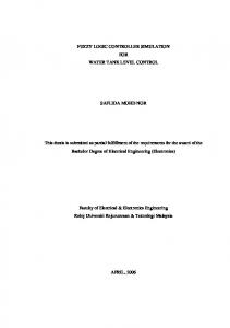
Any system which is moving in free space can be described by the six degree of freedom model. The initial model of an AUV constitutes both the kinematics and dynamics of the system. The six degree of freedom modeling is based on Newton Euler axioms as described in [1] and the nomenclature used in this paper is in accordance to SNAME 1950[13]. Two coordinate frames are considered in the modeling of an AUV. The body fixed frame which is assumed to be located in the body of the vehicle and these coordinates are measured with respect to another reference frame which is assumed to fix and known as earth fixed frame or inertial frame.The body fixed frame contains six velocity coordinates representing three translational and three rotational velocities along X, Y and Z direction respectively. The body fixed frame is represented by the vector v=[u v w p q rV

- Yg(U - vr + wq)] =

e

Reduced order modelfor yaw dynamics In this paper we proposed the control design for yaw plane dynamics. For yaw plane maneuvering yaw angle has to be controlled. As shown in Fig. 2, when a rotation of angle tp is given along the Z axis, the X and Y axes are shifted to the new position Xl and Ylrespectively. Therefore we can neglect the out of plane terms to derive the following three term state vector as given in [2] which describe only the yaw plane dynamics.

(I)

1/1 V

y

z

(2)

WhereT)l= [x Y zV are the position coordinates T)z=[1> e 1/1 V are the rotational coordinates.

Figure 2: Yaw Plane Dynamics

and

The linearized equations of motion for yaw plane are represented in matrix form where the vehicle has steady-state speed [1].

[ Figure I: kinematic reference frames for an autonomous underwater vehicle

The mapping between the two coordinate frames is given by the Euler angle transformation Ti = ](T)z)v, where](T)z) is the Jacobian matrix. Based on the Newton's and Euler's equations the six degrees of freedom motion equation for an AUV can be in written in terms of body fixed coordinates:

m[u - vr + wq - Xg (q Z + r Z) + Yg(pq - i") + zg(pr + q)

=

I

Xext

m[v - wp + ur - yg (r Z + p Z) + Zg(qr - v) + Xg(qp + i")

=

I

Yext

m[w - uq + vp - Zg (p Z + q Z) + Xg(rp - q) + yg(rq + v)

Next (3)

WherevJ=[u v wV are the translational velocities and are known as surge, sway and heave velocities and vz=[p q rV are the rotational velocities and are known as roll,pitch and yaw motions.The earth fixed frame consists of six coordinates which represents the position and orientation of the vehicle. The earth fixed frame is represented by the vector T)=[x Y Z 1>

I

=

I

Zext

IxxV + (Izz - Iyy)qr + m[Yg (w - uq + vp) - Zg(V - wp + ur ) ] =

I

Kext

IyyiJ + (Ixx - Izz)rp + m[Zg(u - vr + wq) - Xg (W - uq + vp)] =

I

(m - Yv) (mxG - Nv) 0

�ml+

(mxG - Vi) (Izz - Ni) 0 - Yv (mU - Yr) -Nv (mxGU - Nr) -1 0

[

�l [�H�l

0, (4)

The transfer function for yaw rate 'r' in terms of rudder angle orcan be found by substituting the value of system parameters given in TABLE 1 and by neglecting the out of plane terms from the above three term state vector. It can be expressed by the following equation:

r or

5( -0.482) + (-0.223) 5Z + 5(1.005) + ( 0.119)

(5)

The yaw rate has a stable zero at -0.482 and two real poles at 0.868 and -0.137. The sway dynamics can be obtained by adding one integrator in yaw rate transfer function. It is also known as yaw angle or heading deflection \jf to rudder deflection Or' So the transfer function for yaw angle can be written as: 1/1 or

5(-0.482) + (-0.223) z 53 + 5 (1.005) + 5(0.119) TABLE 1: HYDRODYNAMICPARAMETERS [3]

Mext

(6)

(c)

Sr. No

Parameter

Value

l!nits

1

Izz

3.45

2 Kg.m kg

Added mass

2

Description

COM

Yv

3

Yf

1.93

Kg.mlrad

Added mass

4

Nv

1.93

Kg.m

Added mass

5

Nr

-0.23

2 2 Kg.m /rad

6

Yr

38.37

Kg.mlrad

7

Yv

-68.27

8

Nv

-3.46

A.

control output

Ml along Z axis about

-35.5

m.

Figure 3: Membership Functions for (a) error (b) change in error and (c)

TABLE 2: CONTROL

e

NL

NM

RULE BASE

NS

ZE

PS

PM

PL

Ae

Cross flow drag

NL

NVL

NL

NL

NL

NM

NS

ZE

Cross flow drag

NM

NL

NL

NL

NM

NS

ZE

PS

Kg.m

Cross flow drag

NS

NL

NL

NM

NS

ZE

PS

PM

Kg

Cross tlow drag

ZE

NL

NM

NS

ZE

PS

PM

PL

PS

NM

NS

ZE

PS

PM

PL

PL

PM

NS

ZE

PS

PM

PL

PL

PL

PL

ZE

PS

PM

PL

PL

PL

PVL

2

DESIGN OF PROPOSED CONTROL

Fuzzy logic based control design

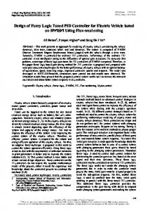
Fuzzy logic based control design doesn't depend on system model accuracy while it is based on human experience. This phenomenon is very useful for our consideration because it is very tough to find an accurate model design of an AUV. Tn this paper seven linguistic variable have been used namely NL(negative large), NM(negative medium), NS(negative small), ZE(zero), PS(positive small), PM(positive medium) and PL(positive large) for inputs and two additional fuzzy variable NVL(negative very large) and PVL(positive very large) are used for the control output. Fig.3 indicates the fuzzy variable and their respective triangular membership functions. According to the rule base made, if error is NL and change in error is also NL then the control output will be NVL and if error is NL and change in error is NM then the control output will be NL and so on. The rule base is shown in Table 1.

There are number of defuzzification methods proposed in literature, but in this paper defuzzification has been done by centroid or center of gravity method. The first step of defuzzification typically 'chops off parts of the graph to form trapezoids and all these trapezoids are then superimposed one upon another to form a single geometric shape. Then the centroid of this shape is calculated. The x coordinate of the centroid is the defuzzified value we obtained. With fuzzy controller the response of yaw dynamic system following the trend slowly with high magnitude as compared to set point as shown in Fig.6 (a), but it should be noted that there is a pole at origin which causes the system extremely unstable and we know that the stability is a minimum requirementin control system. So, what we do is shift the pole from origin to slightly towards the left half plane by 0.6 units. This ensures system stability and faster time response.FigA shows a typical STMULTNK block diagram of fuzzy logic controller for yaw plane dynamics.

(a) Figure 4: Simulink implementation for Fuzzy logic controller

B.

(b)

Design of state-feedback gain compensator

The mathematical model of the yaw system was found to have a pole and zero very close to the origin thereby making it closed loop unstable. To stabilize the system, gain compensator was designed such that theEigen values of the closed-loop system are placed in pre-specified positions. This compensator in series with the fuzzy logic controller ensures that the overall yaw plane system achieves the desired dynamic performance objectives. This implementation was possible because the system matrix and the input matrix form a controllable pair. The controllability ensured placement of closed-loop poles anywhere in the left-half of s-plane. Taking into consideration system stability and speed of response the poles were placed on the optimized positions. Ackerman's formula gives us the method of pole placement for required performance.

K

= [0 0 1] M,:-l 4Jd (A)

WhereMcis controllability matrix and 0d (5)is the characteristic equation for closed-loop poles which we then evaluate for 5 = A. The state-space representation of yaw plane of an AUV system is described by:

where

A=

[

x

= Ax

+

C = [0

y = Cx

�]

0

�

[�]

B =

,

-0.119

-1.005 1 o

Bu

-0.482

system matrix

input matrixand

-0.223] output matrix

Steps for assigning the poles using Ackerman's formula are as follows: 1.

Check controllability of the system and find out the controllability matrix

-1.005 1 1.005 1 o

]

o

]

0.891 -1.005 1

0.119 1.005 1

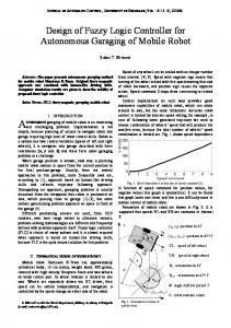
a step input but the system settles at somewhat higher magnitudedue to a pole at origin. So the pole was slightly shifted away from the origin, this ensures the system stability. The pole placement technique provides faster response than fuzzy logic controller, as shown in Fig.6 (d), but there is a cost associated with placing all closed-loop poles because placing all closed-loop poles at desired location requires measurement and feedback of all the state variables of the system which is quit tough task. We have tried pole placement technique for sinusoidal input also but there was a phase lag in the output response so a phase lead compensator was incorporated in the system as depicted in Fig.6 (e). A noticeable improvement in the system response was observed thereafter. To further reduce the phase lag between the input and output a derivative gain was required. However a purely derivative gain is physically not realizable, so a Proportional Derivative controller was used, which reduces the phase lag by 90 degrees. The PD controller is not absolutely essential for the system, because sinusoidal trajectory tracking is achieved even without it, but in cases where accurate tracking is very important, it may be included in the system. The response of the system with fuzzy logic controller coupled with state­ feedback gain compensator is shown in Fig.6 (t). The response time improves considerably as compared to the fuzzy logic controller. The controller shows very good regularity control characteristics and the final output settles at unity, unlike the case of pole placement, where the system settled with a steady state error. � d�e�r-----� to� �th�e �rud 6,-______��������� in �ut

2. Analyse the system parameter which gives the desired performance. Tn this paper, to make the system performance better we have taken( = 0.8 and one of the closed-loop poleis considered at 5 = -2. Hence the desired characteristic equation of closed-loop system we obtain :

53

3.

+

652

[

+

14.255

+

5 ...................

= [4.99

�4 �

........ . .......

·······

f ························ f ·······················

'" Ol

�3 =

12.5 = 0 = 4Jd (5)

14.13

, , , ----------------------- ,j-----------------------j-

A

]

�2 :;:

'" >-

,,

,,

, ,

, ,

_________ L ________________________ L _______________________

Ol 0,

2.74 1.083 0 0 And 4Jd (A) = 9.11 13.33 4.99 14.13 12.5 B y substituting these values i n Ackerman's formula we have calculated the gain matrix K

--

___________

____________ L ________________________ L _______________________

1 O �----------�-----------L----------� o 50 100 150 Timerin seconds).... >

12.5]

( a)

The state-feedback gain compensator associated with fuzzy logic controller is shown in Fig.5.

1.2

· · · · · · · · · · · · · · · · · · · · · · · ·

A

� � '"

Figure 5: State-feedback gain compensator coupled with fuzzy logic controller

TV.

RESULTS AND DISCUSSION

-- Obtained Output , f · · · · · · · · · · · · · · · · · · · · · · -Desired Output

------------� 1 �----------�--��------�

� 0.8 ............ c '=' Q)

g> 0.6

,

, ,

__________ L ________________________ L _______________________

'

I

I

: : ------ -----------------� ------------------------� -----------------------

�:;: 0.4

... .................... � ........................ � .......................

0.2

. ...................... � ........................ � .......................

ro

The procedure detailed in both parts of section TIT was used to obtain simulation results. Theresultsare summarized in Fig.6. The control of yaw dynamics of the underwater vehicle as presented in this paper is difficult due to the system being third order one. Also from analysis it is seen that there are a number of poles and zero near the origin making the controller design difficult. From the graphsobtained, it can be concluded that the fuzzy logic controller produces satisfactory results for

�

: ,

: ,

, , ,

50

, , ,

Time(in seconds)....>

(b)

100

150

1. 2

�

-Y- aw - -ra -t efo r _u _n _i t __ st _ eP in-,-p _ u t _t o _t _ he _r _ ud _ d_er _ __ 'c� � � ,--

__-----, --- Obtained Output

--.... ----------1-----------1---------, , , , , , , , , , , ----------.... ---------- 1 - ----------1 - --------, , , , , , , , , , _________ . L _________ .'. _________ .'. _________ , , , , , , , , , , , , , , ,-----------,-----------------------------, , , , , , , , , , , , , , , , , , ---------- ,... ---------- ----------- ---------, ,

i

A '2

0.8

c o

�

� 0.6 c

0.4

� ." r:' .

--- Desired Output

--------

�

i

Q)

i c =­ '"

0, c

i

---------I, ----------I,-----------I,---------- -.I ----------

05

-

>-

0

>-

-0.2

" ----------" ----------,-----------,----------

__ __ ___ __ __ __ O L� � L_ _L _____' � o 5 10 15 20 25 30

-0.4 '-------'--'--' 5 20 15 25 30 o 10

Time(in seconds)---->

Time(in secod n s)---->

(c)

(f) Figure 6: (a) Yaw angle control with fuzzy logic control having a pole at origin (b) Yaw angle control for fuzzy logic control by shifting the pole from origin (c) Yaw rate for unit step to the rudder (d) Yaw angle control with pole

Yaw response

7�

for unit step inp ut to the rudder -;-�--;- �====�====� u ut = t t

placement design (e) trajectory tracking with pole placement and compensator (f) Step response for fuzzy logic with state-feedback gain compensator

----

6

_____ _ _ _ _

�------------�-------------I

1, \ f\ : �4 --v �- - ;

-w-

--

�3

�2

-

:

:

----------

I

c

; -----------!- -----------� --

-- --

-

I

I

---------

I

, , ,

- - - - - - - - - - - � - - - - - - - - - - - _..I. ___________ •.• _ _ _ _ _ _ _ _ _ _ _ .L. ___________ I I I I

,

'" >-

�

5 H-�----�------�------�--------�----� :

'1:i

01 c

�::�;::�� :�

, ,

----------- , ------------.,-------------, ------------ 1"" ----------I

---------

,

I

--- I ---------I

I

,

---------------, , I

I

, ,

I------------- -I

I

I

,

, , ,

----------

CONCLUSION

Tn this work a new technique is adopted for designing a controller by combining the analytical feedback control with fuzzy control. From results and discussion, the performance of the approach appeared to be better as compared to only fuzzy control and stand-alone state feedback control. However, the desired performance was achieved as the model of the system was strongly controllable and observable and also eliminatesthe impulse modes by shifting the closed-loop poles to the specified locations.

I

Tlme(m seconds)---->

. 4.

V.

O L-----�-----L--�--� 6 o 2 8 10 (d)

---' 1.5i--;-------t----;--'-----;;::======;_] Yaw response for unit step input to the rudder

VI.

ACKNOWLEDGEMENT

We would like to thank Dr. Chandrasekhar, Director CSTR­ CEERT Pilani, for his support and encouragement which led to the completion of this work. The authors thank their colleagues at Electronic control system lab, CSTR-CEERT Pilani. REFERENCES [I]

ThoLT.Fossen "Guidance and Control of ocean vehicles'''Wiley,New York,1994.

1

[2]

Timothy Prestoro "Verification of a Six-Degree of Freedom for the Simulation

�

of

REMUS

Autonomous

Underwater

Vehicle",Massachusetts Institute of Technology,November 200 I.

� "0

[3]

c

Nag,

A; Patel, SS; Akbar, SA, "Fuzzy logic based depth control of an

autonomous

underwater

vehicle,"

Communication, Control and

in

Automation,

Computing,

Compressed Sensing (iMac4s),

2013

International Multi-Conference on , voL, no., pp.117 -123, 22-23 March 2013 doi: 10.1109/iMac4s.2013.6526393. [4]

Rentschler,

ME;

Hover,

F.S.;

Chryssostomidis,

C,

"System

identification of open-loop maneuvers leads to improved AUV flight

- 1.50L------:'-------,L:----,L------:2,LO------2L-:: 5------='03

performance," in Oceanic Engineering, IEEE Journal of , voUI, no.I, pp.200-208, Jan. 2006 doi: 10.1109/JOE.2005.858369. [5]

Pan-Mook Lee; Seok-Won Hong; Yong-Kon Lim; Chong-Moo Lee; Bong-Hwan Jeon; Jong-Won Park, "Discrete-time quasi-sliding mode control of an autonomous underwater vehicle," in Oceanic Engineering,

(e)

IEEE

Journal

of

,

voL24,

no.3,

pp.388-395,

Jul

1999

doi:

10.1109/48.775300. [6]

Healey, AJ.; Lienard, D., "Multivariable sliding mode control for autonomous diving and steering of unmanned underwater vehicles," in Oceanic Engineering, IEEE Journal of , voU 8, no.3, pp.327-339, Jul 1993 doi: 10.1I09/JOE.I993.236372.

[7]

Santhakumar, M.; Jinwhan Kim, "Modelling, simulation and model reference

adaptive

control

of

autonomous

underwater

vehicle­

manipulator systems," in Control, Automation and Systems (ICCAS), 2011 11th International Conference on , vol., no., pp.643-648, 26-29 Oct. 2011. [8]

Santhakumar, M.; Asokan, T., "Coupled, non-linear control system design

for

autonomous

Automation,

Robotics

underwater and

Vision,

vehicle 2008.

(AUV)," ICARCV

in

Control,

2008.

10th

International Conference on , vol., no., pp.2309-2313, 17-20 Dec. 2008 doi: 10.l109/ICARCV.2008.4795893. [9]

Amjad, M.; Ishaque, K.; Abdullah, S.S.; Salam, Z., "An alternative approach to design a Fuzzy Logic Controller for an autonomous underwater vehicle," in Cybernetics and Intelligent Systems (CIS), 2010 IEEE Conference on , vol., no., pp.l95-200, 28-30 June 2010 doi: IO.ll09/1CCIS.20 I 0.5518556.

[10] Smith, S.M.; Rae, GJ.S.; Anderson, D.T., "Applications of fuzzy logic to the control of an autonomous underwater vehicle," in Fuzzy Systems, 1993., Second IEEE International Conference on , vol., no., pp.10991106 vol.2, 1993 doi: 10.1109IFUZZY.1993.327361. [II] Innocenti, M.; Campa, G., "Robust control of underwater vehicles: sliding mode vs. LMI synthesis," in American Control Conference, 1999. Proceedings of the 1999 , vol.5, no., pp.3422-3426 vol.5, 1999 doi: 10.1 109/ACC. I 999.782400 [12] Liuji Shang; Shuo Wang; Min Tan, "Fuzzy logic PID based control design for a biomimetic underwater vehicle with two undulating long­ fins," in Intelligent Robots and Systems (IROS), 20 I0

IEEEIRSJ

International Conference on , vol., no., pp.922-927, 18-22 Oct. 20 I0 doi: 10.1109ITROS.2010.5652459. [13] Shahriar

Negahdaripour,

"Controller nonlinear

design

for

obserbers",

Sohyung an

Cho

autonomous

International

and

Joon-Young

underwater

Journal

of

Kim,

vehicle Ocean

using System

Engineering I(I) (20 II) 16-27 001 I0.6674ITJOSE.20 11.1.1.0 16. [14] Hydromechanics Subcommitte,"Nomenclature for treating the motion of a submerged body through a fluid", Report of the American Towing Tank Conference published by Society of Naval Architects and Marine Engineers (SNAME), New York, USA, April, 1950. [15] Tadahiro Hyakudome, "Design of Autonomous Underwater Vehicle", Japan Agency for Marine-Earth Science and Technology (JAMSTEC), Japan, Vol. 8, No. I (20 II) ISSN 1729-8806, pp 122-130.