configurable systems digital signal processing, multime- .... PAD. 1 0 ... Figure 5. General format of register instructions. OPCODE .... Multicast Signature:.
A Dynamically Reconfigurable Weakly Programmable Processor Array Architecture Template ∗ Dmitrij Kissler, Frank Hannig, Alexey Kupriyanov, and J¨urgen Teich Department of Computer Science 12, Hardware-Software-Co-Design, University of Erlangen-Nuremberg, Germany Abstract As modern areas of application for coarse-grained reconfigurable systems digital signal processing, multimedia in embedded devices, and wireless communication can be mentioned among others. These fields include different algorithms with varying complexity and speed requirements. In this paper a new highly parameterizable coarse-grained reconfigurable architecture called weakly programmable processor array is discussed. It consists of several weakly programmable processing elements with a VLIW (Very Large Instruction Word) architecture which are connected with the help of dynamically reconfigurable interconnect modules.
1
Introduction
Recent advances in the semiconductor technology allow the hardware designer to integrate several complex modules like processors, peripheral devices, and memory in a single System-on-a-Chip (SoC). A high level of reconfigurability and parallelism plays an increasingly important role in modern hardware systems. In particular, the embedded systems for digital signal processing have to be very flexible and implement different signal processing standards at once. The embedded systems for wireless communication, for example, usually implement multiple wireless communication protocols. Reconfigurable system architectures can be classified with the help of the single processing units functionality and the width and configurability of the interconnect [2,12]. The basis of the currently available fine-grained reconfigurable architectures build the so called lookup tables (LUTs), which can be configured to implement different logical functions. Lookup tables constitute together with an extremely flexible interconnect network with 1 bit granularity, see Fig. 1, such modern fine-grained reconfigurable architectures like Field Programmable Gate Arrays (FPGA). The high flexibility of the interconnect network has the dis∗ Supported in part by the German Science Foundation (DFG) in project
under contract TE 163/13-1.
advantage to be very inefficient in terms of area usage. Up to 80 % of the total die area on a typical commercial FPGA is devoted to interconnect [11]. Another undesirable impact of the fine-grained interconnect schemes is that on the computational complexity of placement and routing algorithms, as well as the big reconfiguration data streams (up to several megabytes in modern FPGAs), and consequently long reconfiguration times [6]. Coarse-grained reconfigurable architectures are especially suited to meet the demands on the computation resources, fast reconfigurability, and flexibility, as well as high power efficency for many reasons. Due to the bigger widths of reconfigurable interconnect signals in coarsegrained architectures, see Fig. 2, much of the routing problems are alleviated [6]. Furthermore, the amount of memory to store different reconfiguration data streams is reduced and consequently the reconfiguration times of the coarsegrained architectures are much smaller. Complex computations can be accomplished in the functional units of the coarse-grained architectures, since these can be complete processors with RISC architecture (Reduced Instruction Set Computer). The object of our research is a new class of massively parallel, reconfigurable, coarse-grained processor architectures called weakly programmable processor arrays (WPPA). This paper is structured as follows: in Section 2 a brief overview of existing coarse-grained architectures is given. Section 3 contains the high-level architectural description of the class of weakly programmable processing elements and arrays we are introducing here. In Section 4 the configuration of weakly programmable processor arrays is discussed. Section 5 gives an overview over the configuration data storage. In Section 6 experimental results are given. Finally, in Section 7 we give an outlook on further research subjects.
2
Related Work
Many different academic and commercial coarse-grained reconfigurable architectures exist. A detailed overview of some of them can be found for example in [6]. Two well-
...
...
Configuration Bit
Figure 1. Fine-grained reconfigurable interconnect [12].
Figure 2. Coarse-grained reconfigurable interconnect.
known commercial coarse-grained architectures are PACT XPP from PACT [1], and Avispa, Moustique, and Bresca IPCores (Intellectual Property Cores) from Silicon Hive [10]. Another examples are D-Fabrix from Elixent [4], the Dynamically Reconfigurable Processor (DRP) from NEC [8], or QuickSilver Technology’s Adaptive Computing Machine (ACM) [9]. Existing fine-grained and coarse-grained architectures have both a lack of programmability in common as a result of own paradigms, which are very different from the von Neumann’s [5]. In coarse-grained architectures different levels of parallelism are utilized. Parallelism at the instruction level is usually accomplished with the help of the VLIW architecture, where several functional units in a single processing element are executing instructions in parallel. Different parallel working processing elements in a coarse-grained architecture build the next hierarchical level of parallelism. Potentially even higher levels are possible, like multiple coarse-grained systems integrated in a high-level array. As an example the Multi-Core streaming arrays from Silicon Hive can be mentioned. Another interesting aspect is the interconnect scheme between different computational units in coarse-grained reconfigurable architectures. Very often static interconnect schemes like meshes or trees are used. Since the interconnect scheme can significantly affect the type of algorithms running on this architecture, the possibility of changing the interconnect structure between the coarse-grained processing units increasingly gains in importance.
ing. For every single WPPE the instruction set is parameterizable at compile time. An example of a weakly programmable processor array is shown in Fig. 3, see also [5].
3
Architecture Description
The base building blocks in our architecture are so-called weakly programmable processing elements (WPPEs). They are called weakly programmable because of the limited instruction memory in each processing element and the optimized control overhead, which is kept as small as possible. The instruction set of a WPPE is also kept small and specific to instructions commonly needed in digital signal process-
3.1
General Structure of a WPPE
Each WPPE can be parameterized at compile time to contain several functional units like adder/subtractors, multipliers, shifters, and modules for logical operations. The number of specific functional units is also parameterizable at compile time. The possibility to add functional units which implement user-defined functions, like for example a FFT (Fast Fourier Transformation) is also provided. Furthermore, a WPPE contains a parameterizable register file for data and also parameterizable register file for control signals. The parameters of both types of register files are the number and width of general purpose and output registers, input FIFOs (First In First Out Buffers) and a new type of FIFO buffer which is called FIFO FB (Feed-Back FIFO). The maximum size of both FIFO types is also parameterizable at compile time. For transfer of data and control signals between the different storage elements like registers and FIFOs a special transfer unit is used. Since we have two types of register files, two types of transfer units exist: one for the transfer of data signals and the other for the transfer of control signals. The FIFO FB are FIFO buffer elements with a feedback of the data output signal to the input of the FIFO FB storage element, see Fig. 4. The data word read in the current clock cycle is automatically written back to the FIFO in the same clock cycle. These elements allow the use of cyclic control and data signals. With the help of FIFO FB the software complexity is further reduced because current read and write pointers are managed in hardware. General purpose and output registers as well as input FIFOs and FIFO FB elements are addressed by the functional and transfer units in the exact same manner. The special functionality of the different data storage elements is only coded by the address of this element in the register file. For the functional and transfer units the special functionality of these storage elements is not visible.
Programmable Interconnection I/O
WPPE
WPPE
WPPE
WPPE
ip0 ip1 ip2 ip3 Input Registers/FIFOs
I/O
WPPE
I/O
I/O
WPPE
I/O
WPPE
WPPE
WPPE
WPPE
General Purpose Regs i0
i1
i2
i3
regI
regGP
WPPE
rPorts
WPPE
WPPE
WPPE
WPPE
WPPE
WPPE
WPPE
WPPE
WPPE
WPPE
WPPE
WPPE
WPPE
WPPE
WPPE
WPPE
WPPE
mux
Instruction Memory
I/O
WPPE
I/O
WPPE
mux
ALU type1
WPPE
WPPE
WPPE
I/O
WPPE
WPPE
I/O
WPPE
I/O
f1
regFlags
wPorts
I/O
I/O
demux
f0 pc BUnit
Output Registers
o0
o1 regO
r0 r1 r2 r3 r4 r5 r6 r7 r8 r9 r10 r11 r12 r13 r14 r15
Instruction Decoder
op0 op1
Figure 3. Example of a weakly programmable processor array. A specific maximum depth dmax is assigned to each FIFO (both types) at synthesis time. At run time, these depths can be dynamically set to values d ≤ dmax to meet applicationspecific requirements. 3.2
Instruction Set Architecture
Five instruction types are defined for use in a WPPE. Register instructions refer to the first type, immediate instructions to the second, and constant instructions to the third type. The fourth type is formed by the move instructions and the branch instructions constitute the last type. The width of each instruction as well as the widths of the internal instruction fields is parameterizable at compile time. With the help of this feature different functional units may have different instruction lengths. This case will usually arise, since the functional and transfer units implement different instruction types. If this fact is taken into account in
Data Input
MUX
FIFO
Write Pointer
Read Pointer
Figure 4. Logical structure of a FIFO FB storage element.
hardware, smaller VLIW programs and consequently faster reconfiguration times result. In Fig. 5 a general format of a register instruction is given. The instructions of this type consist of four internal fields: the Opcode field for the operation code, a field for the address of a destination register Destination Register, and two fields for the addresses of two operand registers: First Operand Register, Second Operand Register. Since this is the general register instructions format, dependent on the width of the register address fields and the width of the operation code some bits may be unused. This is indicated by the Pad field in Fig. 5. The semantics of a register instruction is to write the result of an operation with two operands from the operand registers to the given destination register. Since the length of all instruction types is parameterizable at compile time, the current length is stored in a variable instr width in each functional and transfer unit. The general format of immediate instructions is shown in Fig. 6. Besides a field for the operation code Opcode there is one field for the address of destination register Destination Register, one field for the address of the register with the first operand First Operand Register, and finally a field for an immediate operand Immediate Operand. The semantics of an immediate instruction is to write the result of an operation with the first operand from the first operand register and an immediate operand given by the immediate field to the given destination register. The general format of constant instructions is shown in Fig. 8. The semantics of constant instructions is to load a constant given by the Constant field into the destination register with the address from the Destination Register field. Move instructions have a general format which is similar
Destination Register
OPCODE
First Operand Register
instr_width-1
Second Operand Register
PAD
1 0
... Figure 5. General format of register instructions.
OPCODE
Destination Register
First Operand Register
instr_width-1
Immediate Operand
1 0
... Figure 6. General format of immediate instructions.
to the format of register instructions. The only difference is that in the move instructions there is no second operand and therefore no Second Operand Register field. Instructions of this type can be executed only by the transfer units for data and control signals. The semantics of move instructions is to copy the data from the register with the address given by the First Operand Register field into the destination register with the address given by the Destination Register field. 3.3 Multiway Branch Unit For VLIW architectures very often multiway branch units are used [7]. Since a WPPE has a VLIW architecture this approach was also chosen here. The general structure of our implementation of a multiway branch unit is depicted in Fig. 7. With the help of a parameterizable number of branch flags a multiplexer for the selection of several branch target addresses is controlled (Branch Target Multiplexer in Fig. 7). As a branch flag for the Branch Target Multiplexer any control signal from the register file for control signals, input control signals or any status flag from any functional unit for addition/subtraction can be chosen. This is coded in the Selects For The Branch Flag fields in the currently decoded branch instruction from Fig. 9. The different branch target addresses are also given in the
Adder Flag F i-1
CntrlRegs
CntrlInputs
...
...
BRANCH FLAG MUX ... 1 0
Adder Flag F ...
i-1
CntrlRegs
CntrlInputs
...
...
Last Branch Address
3.4
Dynamically Reconfigurable Interconnect Wrapper
BRANCH FLAG MUX ... 1 0
Last Branch Flag
First Branch Flag
branch address fields of the branch instruction from Fig. 9. Each functional unit for addition/subtraction generates four status flags which give additional information about the result of the last operation in this functional unit. The following status flags are generated: the Carry flag is set if a carry bit was generated during the last operation, the Overflow flag is set if an operand overflow occurred, the Negative flag is set if the result of the operation was negative, and finally the Zero flag is set if the result of the last operation was equal to zero. The different status flags from potentially several functional units for addition/subtraction are chosen with the help of additional multiplexers which are not shown in Fig. 9. With the help of this concept n branch flags are analyzed in parallel and a total of 2n different branch target addresses can be given by only one branch instruction in a cycle. Two values for the operation code can be given: Next and Branch. In case of Next instruction the program counter of a WPPE is simply incremented by one. If Branch is chosen the described multiway branch mechanism is activated and depending on the values of the select signals for the Branch Flag Multiplexers in Fig. 7, the select signals for the status flag multiplexers (not shown in Fig. 7), and the actual values of the signals selected as branch flags the program counter is set to the appropriate target address.
First Branch Address ...
i-1 BRANCH TARGET MUX ... 1 0
Branch Target
Figure 7. Logical structure of a multi-way branch unit in a WPPE.
An interconnect wrapper encapsulates the corresponding weakly programmable processing unit and is used to implement different interconnect topologies. Different topologies between the single WPPEs in a weakly programmable processor array like honeycomb, fat tree, and others can be implemented and changed at run-time. To define all possible interconnect topologies, an adjacency matrix is given for each interconnect wrapper in the array at compile time. The structure of the adjacency matrix is exemplary
OPCODE
Destination Register
Constant
instr_width-1
1 0
... Figure 8. General format of constant instructions.
OPCODE
Selects for the first branch flag
&
...
&
Selects for the last branch flag
j-1
first branch address
&
...
&
last branch address
2 1 0
...
Figure 9. General format of branch instructions. shown in Fig. 10. All input and output signals in the four directions N (north), E (east), S (south), and W (west) of the interconnect wrapper, as well as input P in and output signals P out of the encapsulated WPPE are organized in a matrix form. The input signals of the interconnect wrapper and the output signals of the encapsulated WPPE build the rows of the corresponding adjacency matrix, and the output signals of the interconnect wrapper and the input signals of the encapsulated WPPE build the columns of the interconnect wrapper module. There are two input and output signals in each direction of the interconnect wrapper and two input and output ports in the encapsulated WPPE for the corresponding example interconnect wrapper for the adjacency matrix in Fig. 10. If an arbitrary input and output signal have to be connected the variable c in Fig. 10 is set to 1. Otherwise it is set to 0. If many input signals are allowed to drive a single output signal a multiplexer with approj
N out
E out
i
S out
P in
W out
·
N in
· ·
E in
· ·
S in
·
·
·
cij
·
·
·
·
·
·
W in
· ·
P out
· ·
cij ←
1, if ∃ a possible connection between input and output ports, 0, otherwise;
Figure 10. Adjacency matrix example.
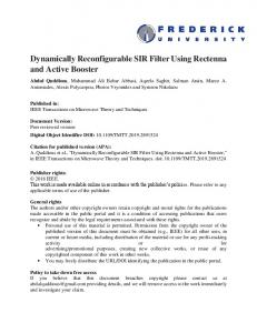
priate number of input signals is generated. The inputs of this multiplexer are connected to the corresponding input signals and the output to the corresponding output signal. The logical structure of an interconnect wrapper module is schematically shown in Fig. 11. The select signals for such generated multiplexers are stored in configuration registers and can therefore be changed dynamically. By changing the values of the configuration registers in an interconnect wrapper component different interconnect topologies can be implemented and changed at run-time. The number and width of the input and output signals of the interconnect wrapper component might be different. This is configured at compile time. 3.5
Weakly Programmable Processor Array
The interconnect wrapper components of each weakly programmable processing element is connected in a regular grid topology to form a weakly programmable processor array. Two levels of connections can be specified. The regular static connections between the single interconnect wrapper components build the first level. The second dynamic level is the current interconnect topology which is defined by the values of the configuration registers. By means of the first static level of interconnect signals the problems in placing and routing of WPPEs in an array are reduced. With the help of the second level different interconnect schemes can be changed dynamically. To achieve dynamic reconfigurability of VLIW programs and interconnect structure each WPPE has a small configuration loader component. A configuration loader is controlled by a finite state machine. Additionally, there is a global configuration controller and global memory for storage of different configurations on the WPPA level. The global configuration controller is connected to an external control unit. This can be for example an embedded processor core in a SoC design. In a configuration or reconfiguration phase the global configuration controller reads the current configuration
Column: 2 1 0
NORTH input
NORTH output
Vertical Mask Register (V)
MUX
...
E
W
WPPE data output S
...
MUX
Interconnect Wrapper
Bit # 2
ICN Wrapper
Bit # 1
ICN Wrapper
ICN Wrapper
ICN Wrapper
ICN Wrapper
ICN Wrapper
Reconfiguration Scheme
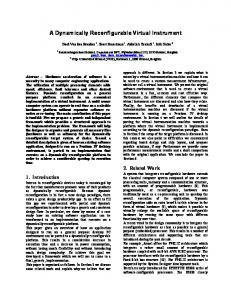
For the configuration and reconfiguration of a WPPA a multicast scheme called RoMultiC (Row Multicast Configuration) was chosen [13]. This method also allows for partial reconfiguration of a weakly programmable processor array. There is a corresponding multicast bit for each row and each column in a two-dimensional processor array. Every interconnect wrapper in the processor array is connected to one horizontal and one vertical multicast bit, see Fig. 12. If a multicast bit is set the corresponding row or column in
V: 0 1 1
V: 1 1 1
Figure 12. Multicast configuration of the single processing elements and their interconnect modules.
Figure 11. Logical structure of the reconfigurable interconnect wrapper module.
4
ICN Wrapper
Multicast Signature: H: 0 0 1
SOUTH output
from the global configuration memory and puts the data on a global configuration data bus. The width of the global configuration memory and the configuration data bus are parameterizable at compile time. They may be different from the width of local VLIW instruction memories and the width of configuration registers in the single WPPEs and interconnect wrapper components. The local configuration loader modules in WPPEs which have to be configured run synchronously with the global configuration controller and write the received configuration words to the respective storage elements. To achieve scalability of weakly programmable processor arrays a multicast scheme was chosen. With the help of multicast bits in special registers it is possible to address single processing elements as well as groups of processing elements in an array. This scheme is explained in detail in Section 4.
ICN Wrapper
ICN Wrapper
Configuration Bit
SOUTH input
Bit # 0
Multicast Signature: H: 1 1 0
Bit # 0
WPPE N
Horizontal Mask Register (H)
WEST config reg.
SOUTH config reg .
WPPE_IN config reg .
...
MUX
WPPE data input
EAST output
...
Bit # 1
Row: 0 1 2
EAST input
NORTH config reg .
MUX
...
WEST output
EAST config reg.
MUX
WEST input
Bit # 2
the array is selected. Now those WPPEs will be configured which have both the vertical and horizontal multicast bits set. The single multicast bits are grouped into two multicast registers: a vertical mask register for the columns of the array and a horizontal mask register for the rows of the array. Both mask registers are located in the global configuration controller and are accessible from an external control unit. For the tuple of two mask register values we use the term multicast signature. A multicast signature uniquely identifies a group of weakly programmable processing elements. This includes the case of a single processing element as well as processor array as a whole.
5
Reconfiguration Data
The global configuration memory contains the different configurations, i.e. VLIW programs and interconnect schemes. A VLIW program and an interconnect scheme are grouped to build one configuration type. Since configuration memory consumes logic resources it has to be as small as possible. Therefore in a WPPA a possibility is given to address the VLIW program configuration and interconnect scheme separately. Then this combination of VLIW program and interconnect scheme does not have to be stored as a separate configuration type. The width of the global configuration memory is parameterizable at compile time. It is independent of the width of the VLIW memories in the single processing elements of the array, since they all can be different on their part. This helps to control the reconfiguration time of the processor array, its scalability, and flexibility. If a small width for
the configuration memory is chosen, multiple configuration words have to be read to construct a single VLIW instruction. On the other side, a very wide global configuration data bus consumes more power and chip area. Therefore a tradeoff between the scalability and configuration speed has to be made. A higher flexibility can be achieved if the VLIW memories and configuration registers for the interconnect scheme can be configured separately. If for a new application the current interconnect scheme has to be changed but the programs may stay the same, only the much smaller interconnect data has to be configured. This approach corresponds to the differential reconfiguration of the processor array.
6
Case Study
A highly parameterizable template for the generation of weakly programmable processor arrays was written in VHDL (Very High Speed Hardware Description Language). An example array with four WPPEs was instantiated and tested on a Xilinx Virtex-II Pro TM xc2vp30 FPGA. As functional units all processing elements have two adder modules, one multiplier module, two modules for the transfer of data, and one module for the transfer of control signals. Data path width was chosen to be 16 bit. Each WPPE has 2 Kbyte local memory. The maximum operating frequency for this design is 84 MHz. Furthermore, it was integrated in a SoC-Design with an embedded P OWER PC-Core as external control unit. The whole SoC-Design uses 54% of the FPGA resources.
7
Conclusion
In this paper a new class of massively parallel embedded processor architectures called weakly programmable processor arrays was introduced. The instruction set architecture and the structure of the single processing elements were described. A novel approach for dynamically reconfigurable interconnection schemes for coarse-grained reconfigurable architectures was also introduced by means of the interconnect wrapper concept. With the help of a special multicast scheme, dynamic and partial reconfiguration schemes can be applied to processor arrays. Besides this architectural research we are currently working on retargetable compilation techniques. An overview how to match the architectural parameters with the mapping methodology is already given in [3]. Furthermore, we develop high-level target-technology independent hardware cost models for single processing elements as well as for the whole processor array. These models include the same parameters as the architecture introduced in this paper. On the basis of such abstract hardware cost models and mapping methodology we want to perform automatic de-
sign space explorations for weakly programmable processor arrays.
References [1] V. Baumgarten, G. Ehlers, F. May, A. N¨uckel, M. Vorbach, and M. Weinhardt. PACT XPP – A Self-Reconfigurable Data Processing Architecture. The Journal of Supercomputing, 26(2):167–184, 2003. [2] Andr´e DeHon. Reconfigurable Architectures for GeneralPurpose Computing. Technical Report A.I. TR No. 1586, MIT AI Lab, Massachusetts, 1996. [3] H. Dutta, F. Hannig, and J. Teich. Mapping of Nested Loop Programs onto Massively Parallel Processor Arrays with Memory and I/O Constraints. In Friedhelm Meyer auf der Heide and Burkhard Monien, editors, Proceedings of the 6th International Heinz Nixdorf Symposium, New Trends in Parallel & Distributed Computing, volume 181 of HNIVerlagsschriftenreihe, pages 97–119, Paderborn, Germany, January 2006. [4] Elixent Ltd. Product Overview. http://www.elixent.com. [5] F. Hannig, H. Dutta, A. Kupriyanov, J. Teich, R. Schaffer, S. Siegel, R. Merker, R. Keryell, B. Pottier, D. Chillet, D. M´enard, and O. Sentieys. Co-Design of Massively Parallel Embedded Processor Architectures. In Proceedings of the first ReCoSoC Workshop, Montpellier, France, June 2005. [6] R. Hartenstein. A Decade of Reconfigurable Computing: A Visionary Retrospective. In DATE’01: Proceedings of Design Automation and Test in Europe, pages 642–649, March 2001. [7] S. M. Moon and S. D. Carson. Generalized Multiway Branch Unit for VLIW Microprocessors. IEEE Transactions on Parallel and Distributed Systems, 6(8):850–862, 1995. [8] M. Motomura. A Dynamically Reconfigurable Processor Architecture. In Microprocessor Forum, CA, 2002. [9] Quicksilver Technology. Product Overview. http://www.qstech.com. [10] Silicon Hive. Product Overview. http://www.siliconhive.com, Eindhoven, The Netherlands, 2004. [11] A. Singh and M. Marek-Sadowska. FPGA Interconnect Planning. In SLIP ’02: Proceedings of the 2002 International Workshop on System-level Interconnect Prediction, pages 23–30, New York, NY, USA, 2002. ACM Press. [12] T. J. Todman, S. J. E. Wilton, O. Mencer, W. Luk, G. A. Constantinides, and P. Y. K. Cheung. Reconfigurable Computing: Architectures and Design Methods. In IEE ’05: IEE Proceedings - Computers and Digital Techniques, volume 152, pages 193–207, 2005. [13] V. Tunbunheng, M. Suzuki, and H. Amano. RoMultiC: Fast and Simple Configuration Data Multicast Scheme for Coarse Grain Reconfigurable Devices. In ICFPT 2005: Conference on Field - Programmable Technology, pages 129–136, 2005.