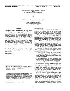
ting is used to render the surfels, honoring the clipping part- ners. This is discussed in Section 3.3. Figure 1 illustrates the rendering setup. 3.1. CSG Operations.
CSG Tree Rendering for Point-Sampled Objects Martin Wicke, Matthias Teschner, Markus Gross ETH Zurich {wicke,teschner,grossm}@inf.ethz.ch Abstract This paper presents an algorithm for rendering of pointsampled CSG models. The approach works with arbitrary CSG trees of surfel models with arbitrary sampling densities. Edges and corners are rendered by reconstructing the involved surfaces separately. The reconstructed surfaces are clipped at intersections. This way, blurring at any magnification is avoided. As opposed to existing methods, which resample surfaces close to object intersections, the proposed approach preserves the original object representation. Since no resampling is needed, dynamic scenes can be handled very flexible. Complex intersections involving any number of objects can be rendered.
1. Introduction CSG operations are among the most important modeling methods. Consequently, the topic has been extensively studied for polygonal meshes, spline patches, or volumetric data. However, little work has been published regarding CSG rendering for point-sampled objects. Point-sampled objects are usually rendered by splatting the individual samples such that each sample contributes its color and depth information to a small area [13]. Each sample is blended with its neighbors. This surface reconstruction method blurs sharp features in texture or geometry. However, a crucial part of CSG modeling is the ability to represent sharp edges, creases and corners. We present an algorithm that allows rendering a CSG tree that combines several point-sampled objects. Samples are considered circular disks, so-called surfels. Surfels belonging to the same primitive object are blended in order to generate a smooth surface, surfels belonging to different objects clip according to the CSG operation applied to the objects. During rendering, clipping partners are identified and the disks are clipped accordingly. Each surfel can be clipped by multiple clipping partners. Clipping is evaluated for each pixel. The main contribution of this paper is a rendering mechanism that is able to render arbitrary CSG trees of pointsampled objects. Sharp features created by the CSG opera-
tions are preserved independent of the magnification level. The original sampling density of the objects can vary arbitrarily, the presented algorithm preserves this sampling. This is an advantage especially in dynamic scenes, where the result of a CSG operation has to be computed for every frame.
2. Related Work The problems arising when rendering objects created by CSG operations have been intensively studied. For polygonal models, references include, but are not limited to [4, 5, 7, 9, 10, 11]. Recently, there has been significant work on pointsampled objects as a modeling primitive [12]. Two publications also address CSG operations [1, 6]. Since the reconstruction mechanism commonly used to render surfaces from point samples blurs edges, the algorithms proposed in [1] and [6] resample the edges created by CSG operations in order to avoid blurring artifacts. Adams and Dutré [1] resample the area around the edges using very small surfels in order to push the blurred area below the pixel area. This method is fastest, but can never completely conceal the point-sampled nature of the edge. Magnifying the edge will result in blurring. Pauly et al. [6] introduce a special surfel class that explicitly represents an edge. This surfel carries two normals, and is rendered as two clipping surfels with identical centers. This surfel is moved onto the edge, and the affected area is resampled to fill holes. This method always provides sharp edges, but does not support more complex intersection types like corners. In contrast to [1] and [6], the proposed method does not perform resampling of the surfaces. Zwicker et al. [14] present a hardware renderer for point sampled geometry that can clip surfels with one or more clipping planes. However, when more than two clipping planes affect one surfel, the results are ambiguous. Thus, complex intersections can not be represented with this approach. Our algorithm resolves these ambiguities and correctly renders arbitrarily complex surface intersections.
Our primitives are patches, i.e. point sampled objects without sharp edges. One CSG operation can create objects with sharp edges, two or more might create corners. Our algorithm is able to render these edges and corners with high quality without changing the object representation. In order to represent complex objects, we store a CSG tree T . The leaves of this tree represent patches, the inner nodes store CSG operators. Each inner node thus represents the result of its CSG operation applied to its child nodes. We use the CSG tree to resolve inside/outside tests for complex objects (see Section 3.3). In the remainder of this paper, we use the following notation: for an object A, SA denotes its surface and TA the CSG tree node representing this surface. If A is a primitive, PA denotes the corresponding patch, i.e. the set of surfels representing SA .
CSG Operation edge surfels
surface surfels
find clipping partners splat surfels splat clipped surfels
merge images
Figure 1. Overview of the algorithm. The CSG operation classifies surfels into edge and surface surfels. Edge surfels are passed to our edge rendering algorithm. Surface surfels can be rendered with any point renderer.
3.1.1. Inside/Outside Classification It is common practice to reduce the inside/outside classification for a pointsampled object A to a front-face/back-face test with respect to the closest surfel in PA [1]. In order to determine if a point x is inside A, only its closest surfel s � PA is used for classification. x is considered inside A if its nearest neighbor s does not clip x:
3. Algorithm We present an algorithm capable of rendering sharp edges and corners created by a series of CSG operations applied to point-sampled objects. Surfels that are close to a surface intersection are clipped during rendering. All other surfels are rendered using an arbitrary renderer. The CSG algorithm is modified to classify surfels accordingly (see Section 3.1). Those surfels that need to be clipped are rendered in a two-pass rendering setup. In a first pass, clipping partners are determined, which are stored in lists along with the surfels (see Section 3.2). In the second pass, EWA splatting is used to render the surfels, honoring the clipping partners. This is discussed in Section 3.3. Figure 1 illustrates the rendering setup.
3.1. CSG Operations CSG operations can be reduced to an inside/outside test. Consider two objects A and B with surfaces SA and SB , respectively. The surface resulting from the CSG operation A B is constituted of the parts of surface SA that are inside B combined with the parts of surface SB inside A: SA �
�
�
B
The union operation is analogous: SA �
B
�
�
�
SA B ��� SA B¯ ���
�
SB A � SB A¯ �
(1)
(2)
To improve the readability of the algorithm description, we only consider union and intersection operations. In Section 4, we discuss how to assemble other operations such as difference using intersection and union.
x inside A ��
�
� ��
s clips x x � cs ��� ns
�
0 �
(3)
Here, cs denotes the center, ns the normal of the closest surfel to x in A, and � the dot product. As illustrated in Figure 2 (a), this leads to classification errors. For many applications, these errors are acceptable. However, in our case they would lead to jagged edges. In [6], the MLS projection operator is used to obtain an exact classification. As this method is too computationally expensive to be evaluated several times for each fragment, we remedy the problem by using the two closest surfels s1 and s2 for classification. The inside/outside test according to (3) is performed for both surfels, yielding results in1 and in2 , respectively. These are combined depending on the configuration of the closest surfels: We call two surfels s1 and s2 with centers c1 and c2 concave if s1 clips c2 and s2 clips c1 . Otherwise, they are called convex. Figure 3 illustrates the configurations. We define the inside/outside classification with respect to an object A using the two closest surfels s1 � 2 of a point x: If s1 and s2 are concave, then
x inside A ���� s1 clips x ���� s2 clips x ��
otherwise, if s1 and s2 are convex,
x inside A ���� s1 clips x ���� s2 clips x �
(4)
(5)
Figures 2 (b) and (c) show the effect of our classification method. Note that one can construct situations where even
outside
incorrect inside classification
incorrect outside classification inside
(a)
(a)
(b)
Figure 4. (a) The edge of a cube, with surfels discarded by a conventional CSG operation marked red. Note their contribution to the surface. (b) The cube rendered without these surfels. Holes appear along the edge.
(b)
(c)
Figure 2. (a) Using only the closest surfel for inside/outside classification leads to classification errors. (b) The edge created by an intersection of two differently sampled surfaces, rendered using only the closest surfel for classification. (c) the same edge rendered with our inside/outside test. The yellow surfel is clipped by ten clipping partners.
der point-sampled surfaces [8, 13], samples that contribute to the resulting object are discarded by the CSG operation (see Figure 4). To make sure that the surface can be properly reconstructed, we modify the CSG operation to classify the surfels into four sets instead of two, depending on the surfel radius r and the distance to the the surface of the other object, d. For an arbitrary CSG operation A B, the classification is as follows:
! !
surface surfels: surfels in SA " B, r
c1
c2 (a)
c1
!
inside edge surfels: surfels in SA " clipped, i.e. r # d
c2 (b)
Figure 3. (a) Two concave surfels. Each surfel center c1 � 2 is on the front facing side of the other surfel. (b) Two convex surfels. At least one of c1 � 2 is on the back facing side of the other surfel.
the use of the two closest surfels for classification leads to non-intuitive clipping results containing discontinuities. However, in practice, these situations are very rare, and the resulting artifacts are only noticeable in extreme closeups. Thus, using even more surfels for classification does not justify the additional cost. This problem is also discussed in Section 5.2. 3.1.2. Surface Reconstruction For point-sampled objects, the sets SA and SB are represented as discrete sets of sample points PA and PB . A conventional CSG operation classifies the sample points into two sets: points that are on the resulting surface, and those that are not. Due to the surface reconstruction method used to ren-
�
!
d B
that might be
outside edge surfels: surfels not in SA " B , but close to the edge, so they might contribute to the surface, i.e. r# d outside surfels: surfels that do not contribute to the resulting surface.
Surface surfels can be rendered with any point renderer. Inside and outside edge surfels are rendered using our edge rendering algorithm, outside surfels are discarded. Thus, the edge rendering algorithm handles all point that are close to the edge, i.e. r # d.
3.2. Finding Clipping Partners In a first rendering pass, the edge surfels are splatted into a framebuffer storing a set of surfels C $ x � y% for each cell (pixel), the clip buffer. The clip buffer has the same size as the viewport, and the same viewing and projection transformations are used. Whenever a fragment of a surfel s from patch PA is added � to a clip buffer cell x � y � , it is a potential clipping partner of all surfels t � C $ x � y % belonging to patches PB with PA � & PB .
If s and t are close enough to clip, t is added to the clipping partner list of s and vice versa. We consider surfels close enough to clip if their Euclidean distance is smaller than the sum of their radii. This results in more clipping planes than necessary. However, the computational cost involved in exactly determining whether or not two surfels clip is too high compared to the gain. Function addFragment is a pseudocode version of the procedure. Function addFragment(int x, int y, Surfel s) /* adds a fragment of s to the cell (x,y) */ C ' cellSurfels(x, y); foreach t � C do if (t.Patch � & s.Patch and distance(s, t) < s.r + t.r) then s.addClippingPartner(t) t.addClippingPartner(s)
Function clipped(Fragment x, Object A) /* determine whether fragment x of Object A is clipped */ T ' findNode(A) on ' true while (on �*� isRoot(T )) do T 2 ' getSibling(T ) in ' insideTree(x, T 2 ) T ' T.Father if in = unknown then continue else switch T.Operator case : on ' in case � : on '�� in end while return � on T . At each node, the following operations are applied:
x inside A � 3.3. Clipped Splatting After clipping partners have been determined for all surfels, the surface can be rendered. Clipping is performed during ellipse rasterization. Object space coordinates are computed for each fragment. These are then used to determine whether or not the fragment lies on the surface resulting from the CSG operations as stored in the CSG tree. We consider a fragment x created by a surfel from patch PA . This fragment is part of the surface SA of the object represented by the leaf node TA of the CSG tree. The algorithm has to determine if x is part of the surface of the object represented by the root node of the CSG tree. Therefore, we traverse the tree bottom up, starting at the leaf TA , until the root node is reached. TA and its sibling TB are combined with the CSG operator stored in their father node T ( . To determine whether x lies on the surface represented by T ( , we apply (1) and (2). As x is part of the surface SA , these equations can be simplified to
x � SA � x � SA �
B )� B )�
x inside B �� � x inside B �
(6) (7)
If x is on the surface represented by T ( , we continue up the tree. Otherwise, x can be discarded. Function clipped is a pseudocode version of this algorithm (see also Appendix A). Note that the inside/outside classification can yield the values true, false and unknown. The unknown classification is used if there are no clipping partners to represent a patch. This case is discussed in Section 3.3.1. We now need an insideTree-predicate to determine if a position x is inside the object represented by a CSG tree T . Using the operator stored in T , we can recursively descend into T and thus reduce the problem to finding an inside/outside classification with respect to the leaf nodes of
B �� x inside A B ��
x inside A �� x inside B �� x inside A �� x inside B �
(8) (9)
A pseudocode version of the tree traversal is shown in Function insideTree. The insidePatch predicate implements the inside/outside classification as defined in Section 3.1.1. It is discussed below. Function insideTree(Fragment x, CSGTree T) /* determine whether fragment x is inside or outside the object represented by T */ if isLeaf(T ) then return insidePatch(x, T.Patch) else switch T.Operator case : return insideTree(T.Left) � insideTree(T.Right) case � : return insideTree(T.Left) � insideTree(T.Right)
3.3.1. Unknown Classifications When clipping a surfel s, we can only use clipping partners stored with s, i.e. surfels that have been identified as clipping partners in the first rendering pass. However, during tree traversal, we might need inside/outside classifications for all patches. Not all patches are represented with clipping partners for s. Hence, some inside/outside classifications remain unknown. A pseudocode version of the extended classification including the unknown value is shown in Function insidePatch. An unknown classification does never lead to discarding a fragment (see Function clipped). Consider a fragment x of a surfel s. If the inside/outside classification for x with respect to a patch P cannot be determined, no surfels of P are clipping partners of s, i.e. P does not intersect s. Thus, s is either completely inside or completely outside P. If any of
Function insidePatch(Fragment x, Patch P) /* determine whether x is inside or outside P */ /* find all clipping partners that are part of patch P */ C ' getClippingPartnersOfPatch(x.Surfel, P) switch + C + case 0: return unknown case 1: return � clips(C0 , x) else sortForDistance(C ) if convex(C0, C1 ) then return � clips(C0 , x) �*� clips(C1 , x) else return � clips(C0 , x) �*� clips(C1 , x) the fragments of s needed to be discarded due to P, s would have been discarded entirely by the CSG operation. If the inside/outside classification for a complex object is computed and the classification for one of the involved patches is unknown, we need to deal with unknown as a value in Function insideTree. In order to evaluate (8) and (9), the � and � operators are extended to handle the unknown value: A � unknown A � unknown
�
�
A� A
for all A �-, true � f alse � unknown . . The reason for using these propagation rules is as follows: We check the clipping for a fragment of the surfel s. If the inside/outside classification for patch PA yields unknown, s is not affected by PA . Thus, if PA and PB form a complex object, we can use the classification returned by PB for the combination of PA and PB . Only if the inside/outside status for both PA and PB is unknown, the classification for their combination is unknown as well. Figure 5 shown � an example. Imagine an object defined by the CSG tree A B � C. We consider two surfels s1 � s2 � PC . In order to determine which fragments to discard, we need inside/outside classifications with respect to the ob ject A B. According to the CSG tree, x inside A B /� x inside A 0� x inside B . Because s1 intersects the surfaces of both A and B, this expression can be evaluated for fragments of s1 . s2 does not intersect the surface of B, and the classification cannot be computed. The value of x inside B is unknown. In this case, the classification becomes inde �
� 1
� unknown � pendent of B: x inside A B x inside A x inside A .
PB
s2 s1 PA Figure 5. A cross-section of an object consisting of three patches. The patch PC is parallel to the image plane. The inside is shaded. For s1 � PC , the inside/outside classification with respect to both PA and PB can be computed. For s2 � PC , the classification with respect to PB yields unknown. Thus, the decision which fragments to discard only depends on PA .
ware renderer. That way, no additional rendering pass is needed.
4.1. CSG Operations For point-sampled objects, the inside/outside test is usually implemented using an approximation of the signed distance function. Hence the classification in edge and nonedge surfels is available at no additional cost. Throughout the description of our algorithm we only discussed the union and intersection operations. For pointsampled objects, the inverted object A¯ is obtained by inverting all normal orientations. Using these three operations, any Boolean operation can be assembled. When a CSG tree originally contains other operators than union and intersection, we rebuild it as follows: First, we break other operations down to combinations of union, intersection and inversion. Then, all inversion operations are propagated down the CSG tree until the CSG tree only contains inversion operations at its leaf nodes. At leaf nodes, inversion is achieved by inverting the normal orientation of all� surfels in the patch. Consider for example the� CSG tree A 2 B � C � . Rewriting the 2 operator yields A B � C� � . The inversion is then propagated to the leaf nodes: A B¯ C¯ � , which is an expression that can be evaluated using our algorithm.
4.2. Rendering
4. Implementation We implemented a test application using our algorithm. Surface surfels are splatted using a hardware splatting algorithm presented in [3]. The software-rendered edges are stored in a texture that is merged with the hardware-rendered surfaces in the third pass of the hard-
For software splatting, the algorithm described in [8] is used. The algorithm involves computing the matrix inverse of the splat space to screen space mapping M. When this mapping is close to singular, i.e. when the splat normal is almost perpendicular to the viewing direction, numerical instabilities make the matrix inverse unreliable.
In [8], such splats are discarded. Since they are almost perpendicular to the viewing plane, the resulting artifacts are hardly noticeable. However, we use splatting to determine clipping partners. Missing a clipping plane can result in serious artifacts, independent of the direction of the clipping plane. It is hence imperative that all potential clipping partners are considered. Therefore, we can not simply discard surfels with almost singular M. Instead, a thick line is drawn into the clip buffer, completely covering the ellipse. This might result in clipping partners being added to surfels that do not overlap in the clip buffer. As only the closest surfels are taken into account when computing inside/outside classifications, adding too many clipping partners does not cause any problems. Surfels that are clipping partners although they do not overlap in the clip buffer are never used for an inside/outside decision.
5. Discussion There are two alternative algorithms for edge rendering after CSG operations on surfel-based objects [1, 6]. In contrast to our approach, both rely on resampling. We first discuss both methods before giving a more detailed comparison with our algorithm in terms of speed in Section 5.1. Limitations of our algorithm are discussed in Section 5.2. Adams and Dutré [1] focus on interactive CSG operations. The main focus of the paper is an accelerated inside/outside classification for surfel-based object, so as to achieve interactivity. Sharp edges are drawn by resampling the surfaces close to the edges. The surfels close to the edge are replaced with smaller surfels in order to minimize blending between the two surface parts. Only the closest surfel is used for inside/outside classification, and there can only be one clipping plane per surfel. After the CSG operation is complete, the resolution of the edge is arbitrarily high, but fixed. Zooming on the edge will eventually reveal its blended nature. Pauly et al. [6] also resample the edges after a CSG operation. They use the MLS projection operator for inside/outside classification. After the CSG operation, the edges are resampled as follows: Along the edge, pairs of surfels are identified. Each of these pairs is moved to a point on the edge, and the two surfels are fused into a special surfel storing two normals. This surfel will be rendered as two half-surfels. The holes in the surface that are created by moving the surfels are closed by resampling the affected areas and inserting surfels where necessary. The edge can be refined arbitrarily, and converges toward the edge that would have been created by the CSG operation applied to the MLS reconstruction of the surfel sets, as first defined in [2]. As the edges are created by the special half-surfels, they remain sharp even when zooming in to the edge. When applying more than one CSG operation, the resulting corners
cannot be represented this way. CSG operations between objects with highly different sampling densities pose problems for both algorithms. As noted in [6], these problems can be resolved by upsampling the areas close to edges before the CSG operation. The algorithm presented herein does not resample the edges created by CSG operations. Instead, surfels along the edges are interpreted as circular disks, which are then clipped. That way, we are able to render arbitrary CSG trees applied to point-sampled objects. The sampling density of the participating surfaces can vary arbitrarily. Complex corners or saddle points can be rendered. As a single surfel can be clipped by many others, also very sharp edges and degenerate cases as seen in Figure 7 can be rendered without artifacts. Note that arbitrary corners cannot be rendered with [6] or [14]. Storing several clipping planes per surfel is not sufficient to represent a surface intersection created by a CSG operation. Hence, in [14], corners are generally assumed to be convex: a fragment is discarded if it is clipped by any one of the clipping planes. This is not correct in the general case, see Figure 2 for an example of an edge that is neither convex nor fully concave.
5.1. Performance The costly edge rendering algorithm is only used for surfels close to the edge. The rendering time is thus mainly dependent on the number of viewport pixels covered by edge surfels. Usually, edge surfels only amount for a small fraction of all surfels, and only cover a small portion of the screen. Thus, a timing comparison is difficult, as for conventional renderers, rendering time depends on the total number of surfels and the total number of pixels covered by the model. The following table shows rendering performance for the scenes shown in Figures 7, 8 and 9, at different zoom levels. The timings were taken on a 3GHz PC with a GeForce FX5900 graphics board. Figure
# surfels
7 (b)
1871
# edge surfels 972
8 (a)
20
20
9 (a)
116650
2272
# edge pixels 7189 33404 8763 47469 12234 69450
FPS 9.09 2.63 8.3 2.27 5.55 2.0
The data supports the assumption that rendering time is linearly dependent on the number of visible edge pixels, while the total number of surfels has almost no impact on computation times. The depth of the CSG tree has only minor influence on complexity, as the CSG tree is rarely fully traversed. Spatial coherence can be exploited to further
viewing plane
sB2 sB1
sB0 sA
Figure 6. Artifact created by our classification method. Shown is a union operation on patches A and B. Surfel sA should be clipped at its intersection with sB0 . However, as the center of sB0 is far away, sB1 and sB2 are used for classification of the pixels in question. sA “bleeds” into the surface of B.
speed up the CSG tree traversal. Past results of the traversal can be cached and reused for new fragments with new per-patch classification results. Our two-pass renderer performing edge clipping is significantly slower than a hardware splatter, such as [3]. However, the latter can not perform any edge clipping. One great advantage of [1] is that the resampling process does not result in surfels requiring special treatment. After a CSG operation was applied, the resulting object can be rendered using hardware splatting. The resampling ensures sharp edges up to a magnification at which the surface reconstruction visibly blurs edges created by small surfels. The combined hardware/software rendering presented herein is faster than the software renderer provided with Pointshop3D [6], as long as edges only fill a small fraction of the screen. Rendering times are similar when approximately one fourth of all pixels show edges. Our rendering algorithm offers advantages especially when the rendered scene includes dynamic CSG operations. If the CSG result needs to be computed every frame, edge resampling has to be performed for every frame. Our rendering algorithm can be directly applied after a CSG classification, making a potentially costly resampling step unnecessary. Which algorithm is actually faster highly depends on the scene, setting and view.
5.2. Limitations Using the two closest surfels for classification yields much better results than only using the closest surfel. However, the classification is not perfect. Figure 6 shows a schematic drawing of a situation resulting in an artifact. In order to avoid these artifacts, a smooth surface recon-
struction method like the MLS projection operator has to be used. We chose not to use MLS projection for performance issues (see Section 3.1.1). In practice, such artifacts are very rare. They only occurs if one of the patches is very irregularly sampled. Even then, only singular pixels along the edges are affected and the problem is only visible at large magnifications, and only from very few viewpoints. Note that just as other approaches [1, 6, 14], our method suffers from numerical instabilities. When two clipping surfels are almost coplanar, the frontface/backface test (3) becomes unreliable. This may lead to jagged edges at surface intersections.
6. Conclusion CSG is an important modeling method, that only recently has been implemented for point-sampled objects. We have presented the first general approach to rendering of pointsampled CSG models that preserves the original object representation. It is possible to render CSG trees, including arbitrarily complex edges and corners. Edge rendering is performed by clipping surfels that contribute to an edge. Clipping partners are determined during rendering, preprocessing is limited to the CSG classification. There is no need to change the original object representation in order to display the edges, the edges are not resampled. This is an advantage especially in dynamic scenes, where a CSG operation is computed for every frame. Rendering of arbitrary CSG trees is possible at frame rates comparable to existing software splatting algorithms.
7. Acknowledgements This research is supported by the Swiss National Science Foundation. The project is part of the Swiss National Center of Competence in Research on Computer Aided and Image Guided Medical Interventions (NCCR Co Me).
References [1] B. Adams and P. Dutré. Interactive Boolean Operations on Surfel-Bounded Solids. In Proceedings of Siggraph 2003, pages 651–656, 2003. [2] M. Alexa, J. Behr, D. Cohen-Or, S. Fleishman, D. Levin, and C. T. Silva. Point Set Surfaces. In Proceedings of Visualization 2002, pages 21–28, 2002. [3] M. Botsch and L. Kobbelt. High-Quality Point-Based Rendering on Modern GPUs. In Proceedings of Pacific Graphics 2003, pages 335–343, 2003. [4] H. Chen and S. Fang. A Volumetic Approach to Interactive CSG Modeling and Rendering. In Proceedings of the 1999 ACM Symposium on Solid Modeling and Applications, pages 318–319, 1999. [5] J. Goldfeather, J. P. M. Hultquist, and H. Fuchs. Fast Constructive Solid Geometry Display in the Pixel-Powers Graphics System. In Proceedings of Siggraph 1986, pages 107– 116, 1986.
[6] M. Pauly, R. Keiser, L. Kobbelt, and M. Gross. Shape Modeling with Point-Sampled Geometry. In Proceedings of Siggraph 2003, pages 641–650, 2003. [7] A. Rappoport and S. Spitz. Interactive Boolean Operations for Conceptual Design of 3-D Solids. In Proceedings of Siggraph 1997, pages 269–278, 1997. [8] J. Räsänen. Surface Splatting: Theory, Extensions and Implementation. Master’s thesis, Helsinki University of Technology, 2002. [9] J. Rossignac, A. Megahed, and B. O. Schneider. Interactive Inspection of Solids: Cross-sections and Interferences. In Proceedings of Siggraph 1992, pages 353–360, 1992. [10] N. Stewart, G. Leach, and S. John. An Improved Z-Buffer CSG Rendering Algorithm. In Proceedings of the 1998 Siggraph/Eurographics Workshop on Graphics hardware, pages 25–30, 1998. [11] T. F. Wiegand. Interactive Rendering of CSG Models. Computer Graphics Forum, 15(4):249–261, 1996. [12] M. Zwicker, M. Pauly, O. Knoll, and M. Gross. Pointshop 3D: An Interactive System for Point-Based Surface Editing. In Proceedings of Siggraph 2002, pages 322–329, 2002. [13] M. Zwicker, H.-P. Pfister, J. van Baar, and M. Gross. Surface Splatting. In Proceedings of Siggraph 2001, pages 371–378, 2001. [14] M. Zwicker, J. Räsänen, M. Botsch, C. Dachsbacher, and M. Pauly. Perspective Accurate Splatting. In Proceedings of Graphics Interface 2004, page to appear, 2004.
A. Correctness of Function clipped Function clipped determines whether or not a fragment x created by a surfel belonging to an object A needs to be clipped. The algorithm traverses the CSG tree bottom up, starting at the leaf node representing A. The algorithm always terminates, either if on � f alse, or when the root node is reached. To show the correctness of the algorithm, we use a slightly modified but equivalent version of Function clipped, which simplifies the argument.
1
2 3
Function clipped2(Fragment x, Object A) // determine whether fragment x of Object A is clipped T ' findNode(A) on ' true while ( � isRoot(T )) do T 2 ' getSibling(T ) in ' insideTree(x, T 2 ) T ' T.Father if in = unknown then continue else switch T.Operator case : on ' on � in case � : on ' on ��� in end while return � on
We artificially extend the loop to traverse the tree until we reach the root node, also in case on becomes false.
Hence, the � condition of the while loop is changed to � isRoot T � . The equations
x � x
�
3� B 3�
SA � SA �
B
x � x
�
SA � x inside B �� SA �4� x inside B 5 �
(10) (11)
replace equations (6) and (7) in lines 2 and 3. Note that if x � SA , (6) and (7) are equivalent to (10) and (11). It is easily verified that the above algorithm is equivalent to the one shown in Function clipped. If Function clipped returns f alse, so does the clipped2 function: In this case, the loop terminates when reaching the root node, thus the changed termination condition in line 1 does not change the outcome of the algorithm. When computing a new value for on, on is never false. Therefore, it can be ignored in the conjunctions in lines 2 and 3, leading to the same equations as used in Function clipped. If Function clipped returns true, so does the clipped2 function: In this case, on � true only holds up to some iteration. Before that point, the two algorithms behave identical, as demonstrated above. Function clipped terminates as soon as on � f alse. It is sufficient to show that in Function clipped2, once on � f alse, on is not changed any more. As on itself is one operand of the conjunctions in lines 2 and 3, these always yield f alse. Thus, on � f alse until the root node is reached, and true is returned as required. The algorithm returns � on, therefore it is correct if we can show that
on � true ��
x isOn OT
(12)
is an invariant of the while loop. OT denotes the object represented by the tree node T , x isOn OT means “x is on the surface of OT ”, i.e. x � SOT . This can be easily shown by induction. The condition holds at the beginning of the first iteration: since x is part of a surfel of object A and A � OT due to the initialization of T , x isOn OT ; on is initialized to true. Given that (12) holds at the beginning of some iteration, we show that it also holds at the end. We denote the value of T at the beginning of the loop T1 . Its value at the end of the loop is T ( , the father node of T1 and T2 . Since (12) holds, x isOn OT1 . There are two cases to consider, depending on the inside/outside classification for T2 , i.e. depending on the value of in. 1. If in � unknown, on remains in the same state it was. There are no clipping partners from the object OT2 , hence x isOn OT 6 iff x isOn T1 . Therefore, x isOn OT 6 . (12) holds. 2. If in � true or in � f alse, the value of on depends on the operator stored in T ( . The logic directly follows equations (10) and (11), (1) and which implement (2). Thus, after evaluation, on � true �� x isOn OT , which is the invariant.
(a)
(b)
(c)
(d)
Figure 7. (a) A union of five spheres. (b) The same spatial setup, rotated. The green and cyan spheres are now substracted from the central white sphere. The spheres just touch, thus an extremely thin structure is created. (c) Sampling of the resulting object. (d) Close-up of the spikes. Top: normal view, bottom: sampling.
(a)
(b)
(c)
(d)
Figure 8. (a) An ikosahedron created by the intersection of 20 half-spaces. (b) Sampling. Each face is represented with one surfel. (c) A cube with differently sampled faces. (d) Sampling of the cube: The faces are represented with 1, 25, and 900 surfels, respectively.
(a)
(b)
(c)
Figure 9. (a) A femural head minus two spheres. (b) Closeup of a 3-surface intersection. The edges can be magnified indefinitely without blurring. (c) Sampling. Note the different sampling densities. Surfels are clipped into shape to accurately represent the edges.