A High Performance Massively Parallel Approach for Real Time. Deformable Body Physics Simulation. Thiago Farias, Mozart Almeida, João Marcelo Teixeira, ...
International Symposium on Computer Architecture and High Performance Computing (SBAC PAD 2008) (preprint)
A High Performance Massively Parallel Approach for Real Time Deformable Body Physics Simulation Thiago Farias, Mozart Almeida, João Marcelo Teixeira, Veronica Teichrieb, Judith Kelner Centro de Informática - Universidade Federal de Pernambuco(UFPE) Av. Prof. Moraes Rego S/N, Prédio da Positiva, 1º Andar, Cidade Universitária, 50732-970, Recife-PE Brasil {tsmcf, mwsa, jmxnt, vt, jk}@cin.ufpe.br
Abstract Single processor technology has been evolving across last decades, but due to physical limitations of chip manufacturing process, the industry is pursuing alternatives to sustain computational power growth, including the creation of multi-core systems. Parallel computing targets problems that are scalable and possibly distributed, dividing the problem into smaller pieces. This approach may be explored to satisfy real time constraints required by real time physics simulation. The purpose of this work is to introduce an optimal solution to implement accurate simulation of deformable bodies in real time. This is accomplished through the use of a meshless simulation technique, known as Point Based Animation, implemented using a massive parallel approach provided by NVIDIA Compute Unified Device Architecture (CUDA). Our implementation showed significative improvements on performance in comparison to the former CPU one: impressive speedups of about 20 times could be achieved in the simulation of deformable bodies with 575 physics elements (phyxels) and 53,504 surface elements (surfels).
1. Introduction Single processor technology has been evolving across last decades. For years, programmers have created their applications based on the premise that an enhancement in performance meant a higher clock frequency of operation. Unfortunately, because of physical and architectural bounds, there are limitations on the computational power that can be achieved with a single processor system. Due to physical limitations of chip manufacturing process, chipmakers currently pursue alternatives to sustain computational power growth, including creation of multi-core systems embedded on a chip. One of these implementations can
be found in GPU (Graphics Processing Unit) industry. Since nowadays GPUs are seen as high performance units, this capability made parallel processing paradigm stronger. It demands another type of development, and not every application can take advantage of it. Parallel computing targets problems that are scalable and possibly distributed, dividing the original problem into smaller pieces that will be solved in different places. Several parallel approaches may be used to speed up the solution of a given problem, such as: effective use of multiple cores of a processor (through OpenMP [1], or some third part library); use of a distributed solution (using a middleware, or even a network grid). In case of taking advantage of processor multiple cores, or using a machine with more than one processor, the solution will scale up to the number of cores in the CPU, or the (number of CPUs) x (cores in each CPU). In spite of this solution being not rare, it is not highly scalable, since the newest powerful mainstream processor is a Quad Core [2], which provides a maximum speedup of 4x, if no synchronization pass is needed in the process. Scalability is a key point of the network grid solution. The achieved result is optimal if the problem can be split into independent parts. Although, in case there is any communication between the cells of a grid, the network latency will slow down the entire process. An alternative for making a parallel version of an algorithm is to use a massive parallel computing device as a coprocessor. The GPU can be considered a representative example. Its use for solving problems not related to image generation and rendering, named GPGPU (General Purpose computing on Graphics Processing Unit) [3], is commonly seen for algorithms in the image processing and computer vision areas, and several research areas that can take benefit of massively parallel processing. GPUs usually process
International Symposium on Computer Architecture and High Performance Computing (SBAC PAD 2008) (preprint)
International Symposium on Computer Architecture and High Performance Computing (SBAC PAD 2008) (preprint)
millions of pixels per second through its several pixel shading pipelines (a common high definition video in 1080p resolution has about 2,073,600 pixels at a frame rate of 30Hz, which represents 62,208,000 pixels per second). Although this amazing processing power may be used for general purpose computations, a GPU is not optimized for this function. There are problems intercommunicating the processing parts (implemented in fragment programs). Data can be shared and optimized for reading (through data transformed into textures), but the result of each processing unit computation is only visible outside the scope of the GPU, since it is written in a texture (using a render to texture technique), as well. The time spent with memory transfers between host and GPU is also an issue and is certainly one of the problems to be solved by next generation GPUs. The massive parallel computing approach may be explored to satisfy real time constraints required by real time physics simulation [4]. Simulating the correct behavior of a moving body is a task that can be executed in many ways. Details such as what type of forces will act over the body, granularity of the simulation model, the ability to deform, fracture or return to its rest position, are what make the simulation numerically realistic, and not just visually coherent. Simpler simulation models, like rigid body dynamics, play their role in games and other simulations where the user is mainly looking for visual results, like [5] and [6], for example. When there is a need for accuracy, more complex, time spending physics simulation methods take place, and the real time constraint needs to be forgotten, or at least relaxed.[7] What if we need an accurate method and it has to be interactive? If user needs a precise simulation, the real time constraint will be achieved by parallelizing the solution. A good example of parallel physics simulation is the PhysX engine [8], now being implemented on NVIDIA GPU cards. The main goal of this engine is to provide fast and massive rigid body dynamics simulation, and also some code plates like fluids and deformable bodies. The accuracy of the simulation provided by this engine is sufficient to its primary application, which are games. So, if one seeks for a precise physics simulation, PhysX isn’t yet the correct choice. Since we are interested in complex and precise physics simulation, can it be parallelized by using any physics method? The answer is “yes”. But, the solution will be optimal only if its basic method is widely parallelizable and doesn’t have data dependencies between the simulation elements. Then, what is the
best method for optimizing deformable bodies simulation? Our contribution in this paper is to elect between the most precise, the best method for being implemented in a massive parallel platform, and the implementation itself. We focus on the Point Based Animation method (PBA), previously described in [9]. This paper is organized as follows. Section 2 shows some related work used for comparison reasons with the chosen method. Section 3 describes the reasons to choose PBA as the algorithm to be tested. Section 4 explains some basic concepts of the physics background applied in PBA. Section 5 reports what was done in the implementation of the algorithm, and the results are shown in Section 6. The last section gives some conclusions and suggests what can be implemented as future work.
2. Related work Since the pioneering work of Terzopoulos et al. [10], a lot of techniques appeared with the purpose of simulating deformable objects in various fields of application. In the field of real time applications, some improvement in the calculations were necessary in order to increase the speed of execution, like the works of Müller et al. [5], James and Pai [11], Desbrun et al. [6] and Debunne et al. [12]. In these works there were found ways of overcoming some complexities without visually compromising the behavior of the final simulation. As it can be noticed in both, real time applications and offline simulations, the great majority of the deformable bodies simulation techniques use meshes and connectivity information to simulate volumetric objects, like [13] and [14]. In these works, the simulation is carried on through the creation of tetrahedral meshes, which sometimes can be too complex to execute at interactive rates. The use of connectivity information can be a disadvantage when change of topology is needed, like in [15], [16] and [17], by making extra storage or extra calculation during the simulation. The mesh free or meshless methods shown in [18] and [9] are an alternative to the conventional finite element simulation. In these methods a cloud of points with no connection information enables the more accurate simulation of elastoplastic elements, including change of topology. There is an increasing number of research works trying to optimize the simulation of deformable objects through the use of auxiliary technology, like GPUs.
International Symposium on Computer Architecture and High Performance Computing (SBAC PAD 2008) (preprint)
International Symposium on Computer Architecture and High Performance Computing (SBAC PAD 2008) (preprint)
Works like [19] and [20] use pixel shaders and vertex shaders in order to accelerate the execution of such simulations. Although the positive results, this approach is not fully advantageous because of the programming model offered by the cg [21] interface. Recently, with the popularization of general purpose programming on GPU [3], the execution of general purpose applications became possible through the use of a more suitable programming interface.
plastic and melting objects, supports topological changes, and is render independent (a mesh or a point based rendering method can be used). Moreover, it allows material fine tuning through few parameters, as Young’s modulus and Poisson’s ratio, which govern the material stiffness and volume conservation, respectively.
3. Why PBA?
Unlike mass-spring models similar to the ones described in [23], [24], [6] and [5], finite element models make the simulation of deformable bodies more accurate. This occurs because of, although the computational methods used to simulate them are inherently discrete, the physical models are derived from continuum mechanics [22]. The continuum representation of elastic elements is defined by its equilibrium (or rest) state and certain material properties are specified to describe how the body will react under the application of external or internal forces [25]. When these forces are applied, each element x0i contained in the set of coordinates that sample the rest state of the object are displaced to a new location ui , defining a displacement vector field and consequently specifying the deformation of the object. From the spatial variations (gradient) of that displacement field u i = xi − x0i , it is possible to compute the elastic strain ε of the material. In the linear case (1D), this value is a dimensionless scalar that defines the ratio between the variation of the elongation and the elongation itself ( Δl / l ) . In three dimensions, however, the displacement field assumes the form u i = (u i , vi , wi ) T , where each component can be derived in the three spatial coordinates. Therefore, the strain cannot be expressed by a scalar anymore [23]. In this case, the strain can be represented by a 3 x3 symmetric tensor, shown in Equation 1:
The PBA method [9] was chosen instead of many others because it stands on the continuum mechanics [22], a branch of mechanics that allows us subdividing a body into infinitesimal particles that will have the same properties of the bulk material. The main application domains of this method are problems that deal with dimensions uncontestable greater than the distance between the particles of the material (atoms, molecules and grains). As examples of target problems, we can mention soil mechanics, solid mechanics, fluid mechanics, civil engineering, and so forth. The particle feature inherent to the continuum mechanics approach leads us to describe a body using only discrete particles, without any connectivity, against the finite element method that uses a volumetric mesh to represent the body. This meshless approach is better to be applied in a highly parallelizable environment, since each particle can be processed (calculating internal forces such as strain and stress) in a separate unit, since they need only their pre-computed neighbors information (in the case where plasticity is not considered). Nowadays, there are some physics engines available that support soft body simulation, but while they focus on real time and visually plausible results, the scientific community claims for numerical stability, accuracy and (why not?) real time. The solution given by the PhysX engine is to use a co-processor to perform all the physics calculation. Before, Ageia introduced a PPU (Physics Processing Unit) card. Now, Ageia became part of NVIDIA and continues investing on a parallelizable physics pipeline through the GPU, which works as a physics co-processor. Following the NVIDIA solution, we take the meshless finite element approach of PBA as the better solution to create a radically physically based soft body implementation, which is massively parallelizable and capable of satisfying the real time constraint. Besides the strong physics background, the continuum mechanics approach simulates elastic,
4. Continuum mechanics background
⎡ε xx ⎢ ε = ⎢ε xy ⎢ε xz ⎣
ε xy ε xz ⎤ ⎥ ε yy ε yz ⎥ . ε yz ε zz ⎥⎦
(1)
Typically, the strain is computed using one of the following equations: εG =
(
)
1 ∇u + [∇u ]T + ∇u ⋅ [∇u ]T , 2
(2)
International Symposium on Computer Architecture and High Performance Computing (SBAC PAD 2008) (preprint)
International Symposium on Computer Architecture and High Performance Computing (SBAC PAD 2008) (preprint)
εC =
(
)
1 ∇u + [∇u ]T , 2
(3)
where ε G is known as Green’s nonlinear strain tensor and ε C is the Cauchy’s linear strain tensor, the linearization of ε G [25]. For Hookean materials, the stress σ is linearly dependent of the strain, as shown in Equation 4,
σ = C ⋅ε ,
(4)
where C can be represented by a 6x6 tensor, and for isotropic materials, it assumes the following form shown in Equation 5, depending only on two material dependent values, namely the Young’s modulus Ε and the Poisson’s ratio v : v v 0 0 0 ⎤ ⎡1 − v ⎢ v 1−v v 0 0 0 ⎥⎥ ⎢ ⎢ v v 1−v 0 0 0 ⎥ Ε C= ⎥ 0 0 1 − 2v 0 0 ⎥ (1 + v )(1 − 2v ) ⎢⎢ 0 ⎢ 0 0 0 0 1 − 2v 0 ⎥ ⎢ ⎥ 0 0 0 0 1 − 2v ⎦⎥ ⎣⎢ 0
In a second moment, the code referent to the simulation of physics elements, so called phyxels, was grouped in a module implemented entirely in GPU. Part of the pre-processing step was also implemented in GPU to speed up the pre-simulation phase. The GPU approach was also applied to deform the model’s mesh. In our implementation, we considered only elasticity, without simulating topology changes or plasticity. The mesh is treated as a set of surface elements, called surfels. In our meshes, the surfels correspond to the vertices. The massively parallel approach also matches with the surfels paradigm, which are processed in parallel and in large scales. We chose CUDA (Compute Unified Device Architecture) as supporting architecture because of its easy integration with other C/C++ modules and based on our previous experiences on writing parallel programs [26] [27].
5.1. CUDA (5)
The Young’s modulus describes the elastic stiffness and the Poisson’s ratio defines the volume conservation within the object. After the calculation of the strain and stress, it is necessary to simulate the dynamics of deformable bodies, based on the time dependent coordinates of the elements that compose the object. To accomplish this task, there are a large number of time integration schemes in the literature. The so called explicit schemes are the easiest to implement and the most efficient to execute in real time applications, but are only stable for very small timesteps. The implicit schemes offer better stability, but at terms of computational power and memory consumption they are far more complex [9].
5. Implementation Our first implementation of PBA was focused on the CPU platform (using C++ language), in a way that the physics concepts involved in the simulation were calculated sequentially. The techniques used in the software construction were based on the Müller et al. work [9], following the macro pseudo code shown in [23]. Some modifications were made to the original CPU code to optimize and pre-process some items used along the simulation, such as neighbors, inverse neighborhood and neighbors’ weighting function.
During this section we will discuss the CUDA parallel implementation, and use some specific terms from the architecture, such as kernel, grid, threads etc. For more information about these terms, please refer to the CUDA programming guide [28]. Regarding phyxels’ simulations, the code running in GPU was divided in four kernels: precalcImutableValues, calcStrainStressA, calcStrainStressB and integrate. The first kernel calculates the neighbors’ weighting values (called ω), the inverse moment matrices and the volume of each phyxel. These values are used in the simulation phase of the soft body particles. The Moore-Penrose pseudo inverse algorithm was also implemented on GPU. It is applied on the moment matrices inside the precalcImutableValues kernel. This kernel runs once when the system initializes. The other kernels are invoked at each simulation step. The calcStrainStressA calculates the strain and stress at each phyxel and stores the forces applied by the neighbors in a force vector. Then, calcStrainStressB sums every force stored by the inverse neighborhood and applies it to the correspondent phyxel. The inverse neighborhood comprehends all phyxels that have a certain phyxel “P” as a neighbor. After the force calculation on every phyxel, we use the Verlet [29] integration method to calculate the new displacement for each phyxel. Additional data, such as position, displacement, mass, volume and neighbors’ weighting function are accessed through textures, to guarantee that memory access for these phyxel attributes will occur efficiently,
International Symposium on Computer Architecture and High Performance Computing (SBAC PAD 2008) (preprint)
International Symposium on Computer Architecture and High Performance Computing (SBAC PAD 2008) (preprint)
using texture cache. The tensor that holds the material properties, including isotropy, stiffness and volume conservation is stored in constant device memory, which assures cacheable access to it. As optimization, the floating point multiplications were minimized, and most of the integer multiplications were reduced to 24-bit calculations [28]. The final body structure that holds all the phyxel attributes is as follows: struct CuBody { float *d_positions_masses; float *d_displacements_volume; float *d_forces; float *d_momentMatrices; int numPhyxels; int maxNeighbors; unsigned short *d_neighbors; float *d_omega; float *d_gradui; float *d_lastDisplacements; };
Positions and masses, as well as displacements and volumes were grouped together to form closed 128-bit vectors. This speeds up the reading access because the GPU has specific instructions to load 32, 64 and 128 bits from the global and cacheable memory. Forces and the last displacements are used in the integration step. The gradient of displacement (d_gradui) is intended for calculating the displacement of the mesh and the normals that will be rendered. The d_momentMatrices is a vector in which all 3x3 tensors are stored sequentially. The vector d_neighbors contains the indexes of the phyxels in the neighborhood of a fixed element. Each phyxel can have at most maxNeighbors neighbors. Our CUDA implementation was made for simulating one entire body per kernel invocation, independent of the amount of phyxels. The mesh deformation is applied invoking the updateSurfels kernel. This kernel configuration differs from the simulation ones because the number of surfels is usually much greater than the amount of phyxels. The updateSurfels kernel uses the gradient of displacement for updating the surfel positions, using the passive surfel advection technique, according to the following equation, as described in [9]: u sfl =
1 T ∑ ω( ri )( ui + ∇ui ( x sfl − x i )) . ∑iω( ri ) i
(6)
The result of this equation and therefore the kernel’s output are the surfel displacements, which are
in fact added with the original positions to fill the OpenGL vertex buffer. In this step, the massive parallel architecture is crucial to get impressive speedups because the amount of surfels is much larger than of phyxels.
5.2. Design issues Some design issues occurred because algorithms and data structures, such as sorting and dynamic arrays, are easier to implement in CPU (and in the case of sorting few numbers, it is also more efficient to run them in CPU, as well). Thus, part of the initialization code and neighbor calculation was implemented on the host side. To get the set of neighbors of a given phyxel or surfel, we implemented a spatial hash [30], which has O(1) complexity. The masses of all phyxels are also computed in CPU, since the neighbors need to be sorted to get the average distance to the nearest neighbors. Once support data was calculated using CPU, the rest of simulation was entirely ran in GPU. A great problem found was eliminating the data dependence of the neighbor phyxels. This was achieved by the additional computation of the inverse neighborhood of a given phyxel and splitting the computeStrainStress kernel into two kernels. The communication between the kernels is a sparse matrix containing all forces applied by all phyxels to its neighbors. With this information and the inverse neighborhood, we could calculate the correct forces applied to each phyxel without waiting or polling the neighbors’ threads. This solution has a drawback in the matter of memory. The sparse matrix used to keep the forces grows as a quadratic polynomial 3x 2 and we could have trouble with bodies composed by a large amount of phyxels. For example, a body with 1,000 phyxels would generate 34.33MB of temporary forces, which isn’t an actual problem to the 768MB of memory provided by the NVIDIA GeForce 8800 GTX.
6. Results This section shows the results acquired from the CPU and the GPU implementations of the PBA method. The main parameters that have direct influence to the computational complexity of simulation are maximum neighborhood size and number of phyxels. The maximum neighborhood size and number of phyxels are directly bonded to the complexity, since the expression for it is O((numPhyxels*maxNeighbors) + numPhyxels).
International Symposium on Computer Architecture and High Performance Computing (SBAC PAD 2008) (preprint)
International Symposium on Computer Architecture and High Performance Computing (SBAC PAD 2008) (preprint)
The simulation environment was composed by an Athlon 64 X2 4800+ processor with 1GB RAM and a NVIDIA GeForce 8800 GTX with 768MB GDDR3. All tests were performed in a non biased system, running Windows XP SP2 with the same processes running in background. As input to the simulation, we chose three objects to represent different bodies, having different characteristics, as number of phyxels, topology and density. The first one is an “alien head”, which has 238 phyxels and 16,000 surfels, suspended by its neck, causing a bouncing effect. The second model is a “horn bug” composed by 666 phyxels and 1,460 surfels. The bug was held by one of its legs to cause a pendulum movement, exploring the deformable behavior of its lengthy parts. The third model is a creature, named Dino, with 575 phyxels and 53,504 surfels held by its mouth. Each model is represented by an external mesh and a volume of phyxels. All these information were extracted from models constructed or enhanced using the 3D modeling tool 3D Studio Max [31]. The visual results can be seen in Figure 1, where A, B and C are, respectively, the horn bug, the alien head and the Dino. The dots represent the phyxel cloud that carries the mesh along.
were tested to find the appropriate stiffness behavior and volume conservation for each body. The Poisson’s ratio was fixed in 0.34, which is a midrange value in the domain of this parameter ( [0, 0.5) ). The Young’s modulus varied between 104 N/m2 (for quasi-melting behavior) and 106 N/m2 (for high stiffness). It is important to notice that setting larger values for this parameter may cause unexpected results, due the single floating point precision that is mandatory on GPU implementation.
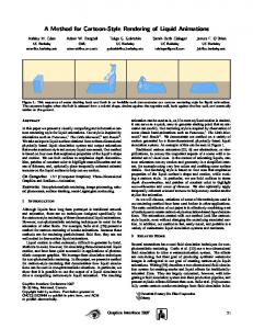
6.2. Performance comparison As we can see in the following charts, there was a noticeable performance improvement that increases with the number of phyxels and surfels. This occurs due the scalability of the GPU solution, which distributes the data along its 128 scalar processors. Figure 2 shows a graphic with the frame rate for a range of objects being processed. In this test, the simulations have from 1 to 10 simultaneous objects updating only its phyxels. In this case, we can notice that even with 10 objects been simulated at the same time, the frame rate is still adequate to real-time applications.
Figure 2. GPU frame rate of phyxel simulation.
Figure 1. Screenshots from the a) “horn bug”, b) “alien head” and c) Dino, showing the phyxels and their correspondent meshes.
6.1. Constant values versus results Values for Young’s modulus and Poisson’s ratio
Another experiment was performed, now also updating the surfel positions to show the deformed mesh. The results are shown in Figure 3, similar to the previous chart. In this scenario, it is possible to observe that only the Dino model couldn’t achieve the ideal frame rate for real time applications. In these two tests, only GPU results were shown. To make a fair comparison, we simulated the same objects in CPU and GPU with the same parameters used in the previous charts. The speedup achieved can be seen in Figure 4 and Figure 5, which show the
International Symposium on Computer Architecture and High Performance Computing (SBAC PAD 2008) (preprint)
International Symposium on Computer Architecture and High Performance Computing (SBAC PAD 2008) (preprint)
frame rate simulating only phyxels and also with the surfels enabled, respectively. Figure 4 and Figure 5 show speedups of 10.05 times for the bug model (higher amount of phyxels) and 20.57 times for the Dino model (higher amount of phyxels and higher number of surfels). For the medium case (alien head) we got a speedup of 24.76 times.
Figure 3. GPU frame rate of phyxel and surfel simulation.
All these results were captured using additional software layers to make easy the replication and configuration of the simulations, as well as the additional OpenGL code to render the model. The absolute running times for all configurations (without the abstraction layers and OpenGL rendering), including surfel updating can be seen in Figure 6.
Figure 6. Running times for the complete simulation using 1 to 10 simultaneous objects.
7. Conclusions and future work
Figure 4. Comparison between CPU and GPU (only phyxels).
Figure 5. Comparison between CPU and GPU (phyxels + surfels).
This paper discussed the use of an efficient, reliable and real time method to make physics simulation for scientific applications (not just focusing visually coherent results). The real time constraint was achieved by embedding the simulation on a massively parallel platform, in this case, the GPU. An appropriate algorithm was chosen due its strong physics base (continuum mechanics) and its intrinsic parallelization. It was implemented using the NVIDIA CUDA architecture and the results showed a very high frame rate, which makes possible to simulate many bodies at the same time with interactive ratios. This fact is only seen in commercial software applied in games with low accuracy algorithms [8]. Impressive speedups were reached: about 20 times for large models (575 phyxels and 53,504 surfels) and about 24 times for the average case (238 phyxels and 16,000 surfels) in our tests. The real time constraint was also enforced in all cases. With 10 simultaneous objects, only the Dino model didn’t reach real time frame rates in GPU. This ratio is very difficult to achieve even simulating only one instance of this model in the counterpart CPU implementation, as seen in Figure 5. As future work, plasticity and fracture may be implemented, as well as interaction using an optimized collision detection and handling.
International Symposium on Computer Architecture and High Performance Computing (SBAC PAD 2008) (preprint)
International Symposium on Computer Architecture and High Performance Computing (SBAC PAD 2008) (preprint)
8. References [1]OpenMP. Available at: OpenMP.org website, URL: http://openmp.org/wp/, last visited: May 2008. [2]Intel® Core™2 Extreme Processor. Available at: Intel® Core™2 Extreme Processor – Overview, URL: http://www.intel.com/products/processor/core2XE/index.htm ?iid=prod_desktopcore+body_core2exQX9770, last visited: May 2008. [3]GPGPU. Available at: GPGPU website, URL: http://www.gpgpu.org, last visited: January 2008. [4]Eberly, D. H., Game Physics, Morgan Kaufmann, 2004. [5]M. Müller, B. Heidelberger, M. Hennix, J. Ratcliff, “Position Based Dynamics”. in proceedings of VRIPhys, Madrid, 2006, pp. 71-80. [6]M. Desbrun, P. Schröder, A. Barr, “Interactive Animation of Structured Deformable Objects”. Conference on Graphics Interface, Morgan Kaufmann Publishers Inc., Kingston, 1999, pp. 1-8. [7]ESI Group, Available at: ESI Group announces the latest version of PAM-CRASH 2G – ESI Group. URL: http://www.esi-group.com/News/PAMCRASH%202G%20V 2007, last visited: January 2008. [8]NVIDIA PhysX. Available at: NVIDIA PhysX website, URL: http://www.nvidia.com/object/nvidia_physx.html, last visited: May 2008. [9]M. Müller, R. Keiser, A. Nealen, M. Pauly, M. Gross, M. Alexa, “Point Based Animation of Elastic, Plastic and Melting Objects”, Symposium on Computer Animation 2004, Eurographics Association, Grenoble, France, 2004, pp. 141151. [10]D. Terzopoulos, J. Platt, A. Barr, and K. Fleischer, “Elastically Deformable Models”, ACM Computer Graphics, ACM Press, jul. 1987, pp. 205-214. [11]D.L. James, and D.K. Pai, “ArtDefo: Accurate Real Time Deformable Objects”, ACM Computer Graphics, ACM Press/Addison-Wesley Publishing Co., Los Angeles, Jul. 1999, pp. 65-72. [12]G. Debunne, M. Desbrun, M.-P. Cani, A. Barr, “Adaptive Simulation of Soft Bodies in Real-Time”. Computer Animation, 2000, pp. 15-22. [13]J.-B. Debard, R. Balp, and R. Chaine, “Dynamic Delaunay Tetrahedralisation of a Deforming Surface”, The Visual Computer, Springer Berlin / Heidelberger, Dec. 2007, pp. 975-986. [14]N. Molino, R. Bridson, J. Teran, R. Fedkiw, “A Crystalline, Red Green Strategy for Meshing Highly Deformable Objects with Tetrahedra”, proceedings of 12 th Int. Meshing Roundtable, Sandia National Laboratories, Sep. 2003, pp. 103-114. [15]J. Brown, S. Sorkin, C. Bruyns, J.-C. Latombe, K. Montgomery, M. Stephanides, “Real-Time Simulation of Deformable Objects: Tools and Applications”, proceedings
of 14th Conference on Computer Animation, Seoul, 2001, pp.228-258. [16]J.-P. Pons, J.-D. Boissonnat, “Delaunay Deformable Models: Topology-Adaptive Meshes Based on the Restricted Delaunay Triangulation”. IEEE Conference on Computer Vision and Pattern Recognition CVPR 2007, June 2007, pp. 1-8. [17]H.-W. Nienhuys, A. F. v. d. Stappen, “Maintaining Mesh Connectivity Using a Simplex-Based Data Structure”. Technical Report UU-CS-2003-18, Institute of Information and Computing Sciences, Utrecht University, The Netherlands. [18] M. Desbrun, M.-P. Gascuel, “Animating Soft Substances with Implicit Surfaces”. ACM SIGGRAPH, 1995, pp. 287-290. [19]G. Ranzuglia, P. Cignoni, F. Ganovelli, R. Scopigno, “Implementing Mesh-Based Approaches for Deformable Objects on GPU”. Fourth Eurographics Italian Chapter, Eurographics Association, Feb. 2006, pp. 213-218. [20]E. Tejada, and T. Ertl, “Large Steps in GPU-based Deformable Bodies Simulation”, Simulation Modelling Practice and Theory, Elsevier, Nov. 2005, pp. 703-715. [21]Cg. Available at: NVIDIA Developer Zone. URL: http://developer.nvidia.com/page/cg_main.html, last visited: May 2008. [22]Fung, Y. C., A First Course in Continuum Mechanics, Prentice-Hall, Inc., 1977. [23]Müller, M., Meshless Finite Elements, Point Based Graphics, Morgan Kaufmann Series in Computer Graphics, Elsevier Inc., 2007. [24]A. Nealen, M. Müller, R. Keiser, E. Bozerman, and M. Carlson, “Physically Based Deformable Models in Computer Graphics”, Computer Graphics Forum, Dec 2006, pp. 809836. [25]S. F. Gibson, B. Mirtich, “A Survey of Deformable Models in Computer Graphics”. Technical Report TR-97-19, Mitsubishi Electric Research Laboratories, Cambridge, nov. 1997. [26]Omitted for blind review. [27]Omitted for blind review. [28]CUDA – Compute Unified Device Architecture – Programming Guide Version 1.1. Nvidia Corporation, 2008. [29]T. Jakobsen, “Advanced Character Physics”, Available at: gamasutra.com, URL: www.gamasutra.com/ resource_guide/20030121/jacobson_01.shtml, last visited: January 2008. [30]M. Teschner, B. Heidelberger, M. Müller, D. Pomeranerts, M. Gross, “Optimized Spatial Hashing for Collision Detection of Deformable Objects”, in Proceedings of Vision, Modeling, Visualization VMV 2003, Munich, Germany, Nov. 2003, pp. 47-54. [31]3DS Max. Available at: Autodesk site. URL: http://usa.autodesk.com/adsk/servlet/index?id=5659302&site ID=123112, last visited: May 2008.
International Symposium on Computer Architecture and High Performance Computing (SBAC PAD 2008) (preprint)