computational methods to support this expansion are needed. To understand a biological processes that a living cell undergoes, one has to measure the gene ...
Differential Evolution Algorithms for Finding Predictive Gene Subsets in Microarray Data D.K. Tasoulis, V.P. Plagianakos, and M.N. Vrahatis Computational Intelligence Laboratory, Department of Mathematics University of Patras, GR–26110 Patras, Greece University of Patras Artificial Intelligence Research Center {vpp,dtas,vrahatis}@math.upatras.gr Abstract. the selection of gene subsets that retain high predictive accuracy for certain cell-type classification, poses a central problem in microarray data analysis. The application and combination of various computational intelligence methods holds a great promise for automated feature selection and classification. In this paper, we present a new approach based on evolutionary algorithms that addresses the problem of very high dimensionality of the data, by automatically selecting subsets of the most informative genes. The evolutionary algorithm is driven by a neural network classifier. Extensive experiments indicate that the proposed approach is both effective and reliable.
1 Introduction In modern clinical practice, the correct and accurate treatment of patients heavily depends on diagnoses that incorporate complex clinical and histopathological data. In some cases this task is difficult or even impossible due to the large volume of data and the limited time and/or resources. To this end, fully automated techniques that can assist in the correct diagnoses are of great value. Moreover, as the number of microarray experiments increases constantly, these techniques are becoming more and more a part of personalized healthcare. Thus, robust computational methods to support this expansion are needed. To understand a biological processes that a living cell undergoes, one has to measure the gene expression levels in different developmental phases, different body tissues, and different clinical conditions. Although this kind of information can aid in the characterization of gene function, the determination of experimental treatment effects, and the understanding of other molecular biological processes [7], it also presents new challenges for researchers. Compared to the traditional approach to genomic research, which has been to examine and collect data for a single gene locally, DNA microarray technologies have rendered possible the simultaneous monitoring of the expression pattern of thousands of genes. Unfortunately, the original gene expression data are contaminated with noise, missing values and systematic variations due to the experimental procedure. Several methodologies can be employed to alleviate these problems, such
2
D.K. Tasoulis, V.P. Plagianakos, and M.N. Vrahatis
as Singular Value Decomposition based methods, weighted k–nearest neighbors, row averages, replication of the experiments to model the noise, and/or normalization, which is the process of identifying and removing systematic sources of variation. Discovering the patterns hidden in the gene expression microarray data and subsequently using them to classify the various conditions is a tremendous opportunity and a challenge for functional genomics and proteomics [7]. A promising approach to address this task is to utilize computational intelligence techniques, such as Evolutionary Algorithms (EAs) and Feedforward Neural Networks (FNNs). EAs refer to stochastic optimization algorithms which employ computational models of evolutionary processes. They share the common conceptual base of simulating the evolution of the individuals that form the population using a predefined set of operators. Commonly two types of operators are used: selection and search operators. The most widely used search operators are mutation and recombination. The selection operator mainly depends on the perceived measure of fitness of each individual and promotes natural selection in the form of the survival of the fittest. The recombination and the mutation operators stochastically perturb the individuals providing efficient exploration of the search space. This perturbation is primarily controlled by the user defined recombination and mutation rates. Although simplistic from a biologist’s viewpoint, these algorithms are sufficiently complex to yield robust and powerful search mechanisms, and have shown their strength in solving hard real world optimization problems. FNNs are parallel computational models comprised of densely interconnected, simple, adaptive processing units, characterized by an inherent propensity for storing experiential knowledge and rendering it available for use. FNNs have been successfully applied in numerous application areas. To train an FNN, supervised training is probably the most frequently employed technique. The training process is an incremental adaptation of connection weights that propagate information between neurons. Unfortunately, employing FNNs (or any other classifier) directly to classify the samples is almost infeasible due to the curse of dimensionality (limited number of samples coupled with very high feature dimensionality). One solution is to preprocess the expression matrix using a dimension reduction technique [9, 17]. In this paper, we follow a different approach. EAs and FNNs are employed to discover subsets of informative genes that accurately characterize all the samples. Generally, the aim is to reduce the initial gene pool from several thousand genes (5,000–10,000 or more) to 50–100. Several gene selection methods based on statistical analysis have been developed to select these predictive genes and perform dimension reduction. Those methods include t-statistics, information gain theory, and principal component analysis [4, 8]. It is evident that the choice of feature selection is difficult and bears a significant effect on the overall classification accuracy. Typically, accuracy on the training data can be quite high, but not replicated on the testing data.
Finding Informative Gene Subsets in Microarray Data
3
The rest of the paper is organized as follows. In Section 2 the proposed approach is presented. In Section 3 is devoted to the presentation and the discussion of the experimental results. The paper ends with concluding remarks and some pointers for future work.
2 Algorithms and Methodology To classify samples using microarray data, it is necessary to decide which genes, from the ones assayed, should be included in the classifier. Including too few genes and the test data will be incorrectly classified. On the other hand, having too many genes is not desirable either, as many of the genes will be irrelevant, mostly adding noise. This is particularly severe with a noisy data set and few subjects, as is the case with microarray data. In the literature, both supervised and unsupervised classifiers have been used to build classification models from microarray data. This study addresses the supervised classification task where data samples belong to a known class. EAs are applied to microarray classification to determine the optimal, or near optimal, subset of predictive genes on complex and large spaces of possible gene sets. Although a vast number of gene subsets are evaluated by the EA, selecting the most informative genes is a non trivial task. Common problems include the existence of: a) relevant genes that are not included in the final subset, because of the insufficient exploration of the gene pool, b) significantly different subsets of genes being the most informative as the evolution progresses, and c) many subsets that perform equally well, as they all predict the test data satisfactorily. From a practical point of view, the lack of a unique solution does not seem to present a problem. The EA approach we propose maintains a population of trial gene subsets; imposes random changes on the genes that compose those subsets; and incorporates selection (driven by a neural network classifier) to determine which are the most informative ones. Only those genes are maintained in successive generations; the rest are removed from the trial pool. At each iteration, every subset is given as input to an FNN classifier and the effectiveness of the FNN determines the fitness of the subset of genes. The size of the population and the number of features in each subset are parameters that we explore experimentally. 2.1 The Differential Evolutionary Algorithm Differential Evolution [15] is an optimization method, capable of handling nondifferentiable, nonlinear and multimodal objective functions. To fulfill this requirement, DE has been designed as a stochastic parallel direct search method, which utilizes concepts borrowed from the broad class of evolutionary algorithms. The method typically requires few, easily chosen, control parameters. Experimental results have shown that DE has good convergence properties and
4
D.K. Tasoulis, V.P. Plagianakos, and M.N. Vrahatis
outperforms other well known evolutionary algorithms [15]. DE has been applied on numerous optimization tasks. It has successfully solved many artificial benchmark problems [14], as well as, hard real–world problems (see for example [2]). In [6] DE has been applied to train neural networks and in [10, 11] we have proposed a method to efficiently train neural networks having arbitrary, as well as, constrained integer weights. The DE algorithm has also been implemented on parallel and distributed computers [3, 12]. DE is a population–based stochastic algorithm that exploits a population of potential solutions, individuals, to effectively probe the search space. The population of the individuals is randomly initialized in the optimization domain with NP, n–dimensional vectors, following a uniform probability distribution and is evolved over time to explore the search space. NP is fixed throughout the training process. At each iteration, called generation, new vectors are generated by the combination of randomly chosen vectors from the current population. This operation in our context is referred to as mutation. The outcoming vectors are then mixed with another predetermined vector – the target vector – and this operation is called recombination. This operation yields the so–called trial vector. The trial vector is accepted for the next generation depending on the value of the fitness function. Otherwise, the target vector is retained in the next generation. This last operator is referred to as selection. 2.2 Search Operators The search operators efficiently shuffle information among the individuals, enabling the search for an optimum to focus on the most promising regions of the solution space. The first operator considered is mutation. For each individual xig , i = 1, . . . ,NP, where g denotes the current generation, a new individual i vg+1 (mutant vector) is generated according to one of the following equations: i r2 vg+1 = xbest + µ(xr1 g g − xg ),
(1)
i vg+1 i vg+1 i vg+1 i vg+1
(2)
= = = =
r2 r3 xr1 g + µ(xg − xg ), r2 xig + µ(xbest − xig ) + µ(xr1 g g − xg ), r2 r3 r4 xbest + µ(xr1 g g − xg ) + µ(xg − xg ), r2 r3 r4 r5 xr1 g + µ(xg − xg ) + µ(xg − xg ),
(3) (4) (5)
where xbest is the best member of the previous generation; µ > 0 is a real paramg eter, called mutation constant, which controls the amplification of the difference between two individuals so as to avoid the stagnation of the search process; and r1 , r2 , r3 , r4 , r5 ∈ {1, 2, . . . , i − 1, i + 1, . . . , NP }, are random integers mutually different. Trying to rationalize the above equations, we observe that Equation (2) is similar to the crossover operator used by some Genetic Algorithms and Equation (1) derives from it, when the best member of the previous generation is
Finding Informative Gene Subsets in Microarray Data
5
employed. Equations (3), (4) and (5) are modifications obtained by the combination of Equations (1) and (2). It is clear that more such relations can be generated using the above ones as building blocks. The recombination operator is subsequently applied to further increase the diversity of the mutant individuals. To this end, the resulting individuals are combined with other predetermined individuals, called the target individuals. Specifically, for each component l (l = 1, 2, . . . , n) of the mutant individual i vg+1 , we choose randomly a real number r in the interval [0, 1]. We then compare this number with the recombination constant, ρ. If r 6 ρ, we select, as the l–th component of the trial individual uig+1 , the l–th component of the mutant i individual vg+1 . Otherwise, the l–th component of the target vector xig+1 becomes the l–th component of the trial vector. This operation yields the trial individual. Finally, the trial individual is accepted for the next generation only if it reduces the value of the objective function. One problem when applying EAs, in general, is to find a set of control parameters which optimally balances the exploration and exploitation capabilities of the algorithm. There is always a trade off between the efficient exploration of the search space and its effective exploitation. In [16] a detailed study and experimental results on exploration vs. exploitation issues are presented. In this paper we employed the Equation (1) as a search operator. 2.3 Fitness Function For the proposed system, each population member represents a subset of genes, so a special representation must be designed. When seeking subsets containing n genes, each individual consists of n integers. The first integer is the index of the first gene to be included in the subset, the second integer denotes the number of genes to skip until the second gene to be included is reached, the third integer component denotes the number of genes to skip until the third included gene, and so on. This representation was necessary in order to avoid multiple inclusion of the same gene. Moreover, a version of DE that uses integer vectors has been proposed and thoroughly studied in previous studies [10, 11, 12]. FNNs were used as a classifier to evaluate the fitness of each gene subset. One third of the data set is used as a training set for the FNN and one third is used to measure the classification accuracy of the FNN classifier. The remaining patterns of the data set are kept to estimate the classification capability of the final gene subset. All the FNNs were trained using the Resilient backpropagation (Rprop) [13] training algorithm. Rprop is a fast local adaptive learning scheme, performing supervised training. To update each weight of the FNN, Rprop exploits information concerning the sign of the partial derivative of the error function. In our experiments, the five parameters of the Rprop method were initialized using values commonly employed in the literature. In particular, the increase factor was set to η + = 1.2; the decrease factor was set to η − = 0.5; the initial update value is set to ∆0 = 0.07; the maximum step, which prevents the weights
6
D.K. Tasoulis, V.P. Plagianakos, and M.N. Vrahatis
from becoming too large, was ∆max = 50; and the minimum step, which is used to avoid too small weight updates, was ∆min = 10−6 .
3 Presentation of Experiments In this section we report the experimental results. We have tested and compared the performance of the proposed system on many publicly available microarray data sets. Here we report results from the following two data sets: – The COLON data set [1] consists of 40 tumor and 22 normal colon tissues. For each sample there exist 2000 gene expression level measurements. The data set is available at http://microarray.princeton.edu/oncology. – The PROSTATE data set [5] contains 52 prostate tumor samples and 50 nontumor prostate samples. For each sample there exist 6033 gene expression level measurements. It is available at http://www.broad.mit.edu/cgibin/cancer/datasets.cgi. Since the appropriate size of the most predictive gene set is unknown, DE was employed for various gene set sizes ranging from 10 to 100 with a step of 10. The FNN used at the fitness function consisted of 2 hidden layers with eight and seven neurons, respectively. The input layer contained as many neurons as the size of the gene set. one output neuron was used at the output layer whose value for each sample determined the network classification decision. Since both problems had two different classes for the patterns, a value lower than 0.5 regarded the pattern to belong to class 1 otherwise regarded it to belong to class 2. For each different gene set size the data was partitioned randomly into a learning set consisting of two-thirds of the whole set and a test set consisting of the remaining one third, as already mentioned. The one third of the training set was used by the Rprop algorithm to train the FNNs, and the performance of the respective gene set was measured in the other one third. The test set was only used to evaluate the classification accuracy that can be obtained using the final gene set discovered by the DE algorithm. To reduce the variability, the splitting was repeated 10 times and 10 independent runs were performed each time, resulting in a total of 100 experiments, for gene set size. The classification accuracy of the proposed system is illustrated using boxplots in Figure 1. Each boxplot depicts the obtained values for the classification accuracy, in the 100 experiments. The box has lines at the lower quartile, median, and upper quartile values. The lines extending from each end of the box (whiskers) indicate the range covered by the remaining data. The outliers, i.e. the values that lie beyond the ends of the whiskers, are denoted by crosses. Notches represent a robust estimate of the uncertainty about the median. As demonstrated, using a gene set size of 50–80 for the COLON dataset the algorithm managed to achieve the best results; comparable to those obtained by other approaches [9, 18]. The same is achieved for the PROSTATE dataset for a gene set size ranging from 40 to 60.
Finding Informative Gene Subsets in Microarray Data PROSTATE
100
100
90
90
80
Classification Accuracy
Classification Accuracy
COLON
70 60 50 40
80 70 60 50 40
30 20
7
10
20
30
40
50 60 Gene Set Size
70
80
90
100
30
10
20
30
40
50 60 Gene Set Size
70
80
90
100
Fig. 1. Classification accuracy obtained by FNNs trained using the DE selected gene set for the COLON (left) and PROSTATE (right) datasets.
4 Concluding Remarks In this work we propose an Evolutionary Algorithms approach that maintains a population of trial gene subsets and evolves them to determine which are the most informative ones. At each iteration, every subset is given as input to a Feedforward Neural Network and the effectiveness of the Network determines the subsets that will be maintained in future generations. Experiments on microarray datasets indicate that the proposed approach is effective and reliable. In a future correspondence, we will investigate the performance of the proposed approach when different evolutionary algorithms are employed. We also intend to incorporate unsupervised clustering algorithms in an attempt to implement a system capable of clustering the genes and simultaneously finding the most informative subsets.
Acknowledgment The authors would like to thank the European Social Fund, Operational Program for Educational and Vocational Training II (EPEAEK II), and particularly the Program “Pythagoras” for funding this work. This work was also partially supported by the University of Patras Research Committee through a “Karatheodoris” research grant.
References 1. U. Alon, N. Barkai, D.A. Notterman, K.Gish, S. Ybarra, D. Mack, and A.J. Levine. Broad patterns of gene expression revealed by clustering analysis of tumor and normal colon tissues probed by oligonucleotide array. Proc. Natl. Acad. Sci. USA, 96(12):6745–6750, 1999. 2. M.R. DiSilvestro and J.-K.F. Suh. A cross-validation of the biphasic poroviscoelastic model of articular cartilage in unconfined compression, indentation, and confined compression. Journal of Biomechanics, 34:519–525, 2001.
8
D.K. Tasoulis, V.P. Plagianakos, and M.N. Vrahatis
3. V.P. Plagianakos D.K. Tasoulis, N.G. Pavlidis and M.N. Vrahatis. Parallel differential evolution. In IEEE Congress on Evolutionary Computation (CEC 2004), 2004. 4. S. Dudoit, J. Fridlyand, and T.P. Speed. Comparison of discrimination methods for the classification of tumor using gene expression data. Technical Report 576, Mathematical Sciences Research Institute, Berkeley, CA, 2000. 5. D. Singh et al. Gene expression correlates of clinical prostate cancer behavior. Cancer Cell, 1:203–209, 2002. 6. J. Ilonen, J.-K. Kamarainen, and J. Lampinen. Differential evolution training algorithm for feed forward neural networks. Neural Processing Letters, 17(1):93– 105, 2003. 7. D. Jiang, C. Tang, and A. Zhangi. Cluster analysis for gene expression data: A survey. IEEE Transactions on Knowledge and Data Engineering, to appear. 8. T. Li, C. Zhang, and M.Ogihara. A comparative study of feature selection and multiclass classification methods for tissue classification based on gene expression. Bioinformatics, 20(15):2429–2437, 2004. 9. V.P. Plagianakos, D.K. Tasoulis, and M.N. Vrahatis. Hybrid dimension reduction approach for gene expression data classification. In International Joint Conference on Neural Networks 2005, Post-Conference Workshop on Computational Intelligence Approaches for the Analysis of Bioinformatics Data, 2005. 10. V.P. Plagianakos and M.N. Vrahatis. Neural network training with constrained integer weights. In P.J. Angeline, Z. Michalewicz, M. Schoenauer, X. Yao, and A. Zalzala, editors, Proceedings of the Congress of Evolutionary Computation (CEC’99), pages 2007–2013. IEEE Press, 1999. 11. V.P. Plagianakos and M.N. Vrahatis. Training neural networks with 3–bit integer weights. In W. Banzhaf, J. Daida, A.E. Eiben, M.H. Garzon, V. Honavar, M. Jakiela, and R.E. Smith, editors, Proceedings of the Genetic and Evolutionary Computation Conference (GECCO’99), pages 910–915. Morgan Kaufmann, 1999. 12. V.P. Plagianakos and M.N. Vrahatis. Parallel evolutionary training algorithms for ‘hardware-friendly’ neural networks. Natural Computing, 1:307–322, 2002. 13. M. Riedmiller and H. Braun. A direct adaptive method for faster backpropagation learning: The Rprop algorithm. In Proceedings of the IEEE International Conference on Neural Networks, San Francisco, CA, pages 586–591, 1993. 14. R. Storn and K. Price. Minimizing the real functions of the icec’96 contest by differential evolution. In IEEE Conference on Evolutionary Computation, pages 842–844, 1996. 15. R. Storn and K. Price. Differential evolution – a simple and efficient adaptive scheme for global optimization over continuous spaces. Journal of Global Optimization, 11:341–359, 1997. 16. D.K. Tasoulis, V.P. Plagianakos, and M.N. Vrahatis. Clustering in evolutionary algorithms to efficiently compute simultaneously local and global minima. In IEEE Congress on Evolutionary Computation, volume 2, pages 1847–1854, Edinburgh, UK, 2005. 17. M.E. Wall, A. Rechtsteiner, and L.M. Rocha. Singular value decomposition and principal component analysis. In A Practical Approach to Microarray Data Analysis, pages 91–109. Kluwer, 2003. 18. J. Ye, T. Li, T. Xiong, and R. Janardan. Using uncorrelated discriminant analysis for tissue classification with gene expression data. IEEE/ACM Transactions on Computational Biology and Bioinformatics, 1(4):181–190, 2004.