IEEE TRANSACTIONS ON SYSTEMS, MAN, AND CYBERNETICS-PART
B: CYBERNETICS, VOL. 26, NO. 5, OCTOBER 1996
K. S. Narendra and K. Parthasarathy, “Identification and control of dynamic systems using neural networks,” IEEE Trans. Neural Networks, vol. 1, no. 1, pp. 4-27, 1990. K. S. Narendra and A. M. Annaswaamy, Stable Adaptive Systems. Englewood Cliffs, NJ: Prentice-Hall, 1989. Y. H. Pao, Adaptive Pattern Recognition and Neural Networks. Englewood Cliffs, NJ: Addison-Wesley, 1989, pp. 197-222. Y . H. Pao, S. M. Phillips, and D. J. Sobajic, “Neural-net computing and the intelligent control of systems,” Int. J. Control, vol. 56, no. 2, pp. 263-289, 1992. S. Qian, Y. C. Lee, R. D.Jones, C. W. Barnes, and K. Lee, “Function approximation with an orthogonal basis net,” in Proc. Int. Jointed Conj Neural Networks, San Diego, CA, 1990, pp. 111-605-618. K. Rohani, M. S. Chen, and M. T. Manry, “Neural subnet design by direct polynomial mapping,” IEEE Trans. Neural Networks, vol. 3, no. 6, pp. 1024-1026, 1992. D. E. Rumelhart, Parallel Distributed Processing. Cambridge, MA, MIT Press, 1986. S. Sastry and M. Bodson,Adaptive Control-Stability, Convergence, and Robustness. Englewood Cliffs, NJ: Prentice-Hall, 1989. T . Yabuta and T. Yamada, “Learning control using neural networks,” in Proc. IEEE Int. Con$ Robot. Automat., Sacramento, CA, Apr. 1991, pp. 740-745.
Neural Network Approach for Solving the Maximal Common Subgraph Problem Amin ShouXuy and Mohamed Aboutabl Abstract- A new formulation of the Maximal Common Subgraph Problem (MCSP), that is implemented using a two-stage Hopfield neural network, is given. Relative merits of this proposed formulation, with respect to current neural network-based solutions as well as classical sequential-search-basedsolutions, are discussed.
I[. INTRODUCTION Searching for a best match between two relational structures has been recognized as a fundamental operation since the early works in intelligent information processing applications: Computer Vision [ 11, Structural Pattern Recognition [2], rule-based Expert systems [3], and information retrieval environments [4]. In general, a correspondence can be set between graphs (simple, multi and hypergraphs: directedundirected, labeled/unlabeled) and relational structures. In this paper, we limit ourselves to simple unlabeled graphs. The Maximal Common Subgraph (MCSP) between two simple undirected graphs G l ( V 1 , El) and G2(V2, E 2 ) is obtained by finding two isomorphic subgraphs which contain the largest possible number of edges. Some researchers, like Levi [5] have adopted a weaker definition in which adjacent (nonadjacent) nodes in G 1 may correspond only to adjacent (nonadjacent) nodes in G2. Several attempts have appeared in the literature to solve the MCSP using depth first search combined with backtracking [5]-[7]. Recently, an attempt to solve the graph matching problem using a single-stage Hopfield neural network has been introduced in [8], and
will be referred to as the M&G network. The Hopfield model has been, also, used by several researchers to solv~:the matching problem in some structural pattern recognition problems [9], [lo]. A brief account about the Hopfield model and its uses in solving combinatorial optimization problems, is, first, given below.
A. Hopjield Model a n d Combinatorial Optimization
A Hopfield Network [ 111 is an autoassociative network of artificial neurons with symmetric connections and asynchronous update strategy. The network dynamics converge to a steady state corresponding to a minimum of an energy function and have been described by deterministic [ l l ] , [12] (both discrete and continuous) as well as stochastic equations [13]-[15]. The stochastic formulation draws an analogy between the Hopfield net and some ‘simplemodels (such as the Ising model) of magnetic materials in statistical physics [15]. In these materials, the interactions and dynamics of the atomic magnets are influenced by thermal fluctuations. The idea of a thermallike noise has been fruitful in combining the principle of simulated annealing [16] with the neuronal approach (the Boltzmann machine [13] and the Mean field theory [15]). An Annealed Hopfield model is characterized by binary random decision neurons updated using discrete dynamics: the output of a neuron is always either 0 or 1 but its probability i s a sigmoid function of the form 1/(1 e--2+or*net ) = 0.5 x (1 t a n h ( a * n e t ) ) (1)
The authors are with the Department of Computer Science, Fac-
*
ulty of Engineering, Alexandria University, Alexandria, Egypt (e-mail:
[email protected]). Publisher Item Identifier S 1083-4419(96)05352-6.
+
+
where “a”is a gain factor and “net” is the net input to a neuron. The gain “a” is considered to be inversely proportional to the (pseudo) temperature T . As T approaches 0 the distrihution reduces to a step function. The Mean Field Annealing (MFA) algorithm, at a given temperature, corresponds to a serial relaxation process of the average neural states (mean field vector) [17], [18]. Therefore, tuning of the gain ‘‘a” is equivalent to searching for a critical temperature for annealing [17]. This method is especially useful in escaping from spurious local minima of the energy function and many researchers have applied it to solve combinatorial optimization problems that are characterized by a large number of interacting decisions. The simulation part described in Section IV of the present paper follows the same strategy. B. The M&G Formulation of the MCSP Using the Hopjield Model
The M&G network consists of an array of IV11 x 11/21 neurons, where lVll and (V21 are the number of vertices in G 1 and G2, respectively. Each neuron yZJ computes a decision about mapping node i (from G1) to node j (from G2). Thirj neuron competes with all other neurons in the network such that the largest possible number of edges is obtained in the final common subgraph. M&G formulate the graph matching problem as given in (2) below Min Edges Y /
~ f l
Zfk
+T
Manuscript received December 12, 1992; revised July 25, 1995.
785
JEV2
(
zEV1
)’
Y % J- 1
Y V ( 1 - Y2J)
+2T
(2)
tEVlJEV2
where, {gZi.} and i h , ~ }are the adjacency rnatnces of G1 and G2, respectively. The y and T are positive constants used to fine tune the network operation.
1083-4419/96$05.00 0 1996 IEEE
IEEE TRANSACTIONS ON SYSTEMS. MAN, AND CYBERNETICS-PART
786
B.CYBERNETICS, VOL. 26, NO. 5 , OCTOBER 1996
. . . . . _ _ _ . . _ _ _ _ _ . _ . . . . . . . . . . . . _ weight matrix W fulfills the sufficient conditions for convergence,
Matching
XI1
Network
namely it is symmetric with zero diagonal elements. When this network is left to operate freely, the neurons compete with each other until a steady state is reached at which the local decisions of the neurons are globally consistent with each other, and thus represent the network soluhon to the given edge matching problem. B. The Node Matching Network
.
.
_
_
_
_
_
_
_
_
_
_
_
_
_
_
_
_
_
_
_
_
_
.
_
_
_
_
_
_
_
I
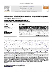
Fig. 1. Two cascaded Hopfield nets to solve the MCSP
It is worth noting that M&G have only considered the direct connection between each pair of nodes when attempting to map them to each other. The surrounding (or local topology) of the graph is not taken into consideration. However, the interneurons connection weights calculations are highly parallel in nature. This feature of the M&G neural solution has motivated the present authors to seek a more powerful neural network which makes use of as much topological information as possible while preserving the independency and locality of the individual neurons decisions and therefore converges to a better solution. This new approach is discussed in Section 11.
This network consists of an array of lVll x IV21 neurons, each of which computes a matching score l c z , E [O, 11 of mapping node i from G1 to node 3 from G2. The node matching problem with its governing constraints can be stated as given in (S), where y1,72,and 7 are positive constants used to tune the network operation.
ifk
j#l
11. THENEW NEURALSOLUTION
In this section, a new formulation for solving the MCSP is proposed. It is based on the use of two cascaded Hopfield networks as shown in Fig. 1. The first network computes the matching scores between the edges of both graphs. The second network, next, computes the matching scores between the nodes. A. The Edge Matching Network
This network consists of an array of lE1l x IE21 neurons, where lE1l and IE2j are the number of edges in G 1 and G2, respectively. Each neuron computes a score ypr t [O, I] representing the strength of the hypothesis that edge p E E l is matchable with edge T E E 2 . The problem of matching as many edges as possible from G1 to edges from G2 can be mathematically formulated as given in (3) below
The last three terms are constraints similar to those of the edge matching network. The first two negative terms represent the trend to fire as many neurons as possible with maximal consistency The following two compatibility measures have been defined a2,,ki E [-1, +l], which reflects the degree of compatibility between mapping node z to node J and, at the same time, mapping node k to node I , and 2) b,, E [-1, +1], which measures the degree of similarity between nodes t and 3 . A discussion of these two measures is given in Section 111. ‘It is worth noting that both of these measures are based on information extracted from the topology of the given graphs, as well as on the results of the edge matching network. The parameters of the node matching network are derived from (4), and can be shown to equal: Iij = 2 7 7 2 b 2 , , wiy,iy = 0,wu,j,;1= -27 (for j # I ) , w,,,kj = -27 (for i # k ) , and W t j , k l = Zyla,,,ki (for i # k and j # I ) . The weight matrix W of this network also fulfills the sufficient conditions for convergence.
1)
+
Min Edges
Y /
C. Results Interpretation
In (3), the first term, with its negative sign, represents the trend to maximize the number of matchable edges. The cpr,qs factor, whose value ranges from -1 to +1, is a compatibility measure reflecting how far the topology of GI, in the neighborhood of edges p and q , is similar to that of G2, in the neighborhood of edges r and s . A detailed discussion of this measure is given in Section 111. The remaining three terms represent the constraints that at most one edge in G1 (G2) matches with any particular edge in G2(G1). T h e y and 7 are positive constants used to tune the network operation. The network energy, as defined by Hopfield [ll], [12], can be stated as
Eventually, the node matching network settles ,down in a local minimal state. The table of the 1c;j final values should be optimally interpreted to decide which nodes are feasibly matchable (a case study is given in Section IV). This is a well-known problem in the field of operations research, and is referred to as the Assignment Problem [20].We have applied the Hungarian algorithm to solve this node assignment problem. 111. EVALUATION OF THE COMPATIBILITY MEASURES Attention is turned now to evaluating the compatibility measures utilized in the design of both networks. A. Edge Matching Compatibility Measure cpr,qs
Comparing (3) and (4),it can be shown that the network parameters are: Ipr = 27,wpr,pr = 0,wpr,qr = -27 (for p # q ) , wpr,ps = - 2 7 (for r # s), and wpr,qs= 27cp,, q s (for p # q and r # s). The
The score cpr,qs measures how far the mapping of edge p to edge r is compatible with the mapping of edge q to edge s. This measure assumes a value of - 1 for full incompatibility, and a value of $1 for full compatibility. Typically, cpr,qsranges between these
IEEE TRANSACTIONS ON SYSTEMS, MAN, AND CYBERNETICS-PART
AA
B: CYBERNETICS, VOL. 26, NO. 5, OCTOBER 1996
BBB
8% Case b
Case a
787
Case c
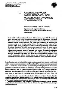
Fig. 2. The three cases of cpr,qs.
H1
\I I \\I
H2
/
/f
K.- - - - - - k'
\&
..
..
$0
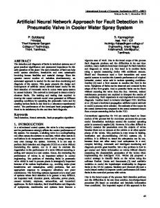
Fig. 3. Evaluation of cpr,qsin Case a two boundaries. Three cases have been encountered when evaluating this measure (Fig. 2). Case a: in which edges { p , q } are incident in G1, and so are edges { T I S } in G2. Case b: in which edges { p , q } are incident in G1 whereas edges { T , s} are not, or vice versa. Case c: in which neither edges { p , y} nor edges { T , s } are incident. In Case a, a subgraph H1 of G1 (Fig. 3), is constructed using the end nodes of edges { p , q } and their direct neighbors. A similar subgraph H2 of G2 is defined around edges { T , s}. The compatibility measure is defined as
1) the number of edges connecting node pairs ( p q l , p q a ) , ( p q 2 ,p 4 3 ) and ( p q 1 ,pya) through exactly one intermediate node. Let these quantities be u t , i = 1,2,3; 2) u4 = 1 if nodes p q and ~ pq3 are direct neighbors, otherwise U 4 = 0; 3) 2,;i = 1,2,3,is the number of edges connected to node p q 2 , excluding those counted in the values of u g ;j = 1,. . . , 4 . The quantities v3;j = 1,.. , , 4 and y z ; i '= 1,. . . , 3 are similarly defined in subgraph H2. In Case b, the edge pair ( p , q ) is fully incompatible with the edge pair ( T , s ) . Hence, cpr,qs
where el(e2) is the number of edges in Hl(H2) (for convenience, neither edges { p , q } nor { T , s} are counted in e l and e z ) ,n12 ( n 2 1 ) is the number of edges in Hl(H2) with no possible match in H2(H1). In order to evaluate 1212, the following quantities are calculated on H1:
= -1.
(7)
In Case c, an almost similar procedure to that of Case a is developed and the value of cpr,qsis given by (6). Example for Castfa): Considering the graphs in Fig. 4, we compute the compatibility of mapping the edge pair ( p = 15, q = 1 2 ) from G1 to the edge pair ( T = 3,s = 2) from G2. The results are shown in the following tables, with x 1 , 2 2 ,arid z3 evaluated at nodes
788
IEEE TRANSACTIONS ON SYSTEMS. MAN, AND CYBERNETICS-PART
B. CYBERNETICS, VOL. 26, NO. 5, OCTOBER 1996
TABLE I
I
I
61 El -15 v1 = 12
TABLE I1
62
12, 10, and 6, respectively, and y1, y2, and y3 evaluated at nodes 1, 5 , and 3, respectively. In this case: el = 13. e2 = 15,nlz = 3,n21 = 5,,and c 1 5 , 3 , 1 2 , 2 = 0.4286. It is worth noting that if we map edge pair (12, 15) to (3, 2) instead, we get a higher compatibility measure equal to 0.857 1. B. Node Matching Compatibility Measure
-
E2 v2 =
az,,kl
This score measures how far the node pair ( i , k ) in G1 is compatible with the node pair ( j , l ) in G2. This measure also has a lower bound of - 1 and an upper bound of + l . Here, we also have encountered the three cases depicted in Fig. 5. The value of a ; j , k l is given by (8), where ypl- is the matching score of edges p and T as computed by the first network. It is worth noting that Case c has no effect on the resulting number of edges, and therefore is considered a neutral case 2yp, - 1 in Case a in Case b . (8) 0 in Case c C Node Matching Compatibility Measure b,, This score also lies in [- 1, +1] and measures the goodness of mapping node z from G I to node 1 from G2 It is defined as in (9), where (see Fig 6) n(7n) is the degree of node z ( J ) , and p,; s = 1,.. . ? n and ~ t t ,= 1,.. . ,m are the edges connected to nodes 7 and J , respectively It is worth noting that b,, decreases with the difference between n and m, whereas it increases with the matching scores among the edges connected to both nodes
I v . RESULTS AND PERFORMANCE EVALUATION We have applied our new algorithm to several case studies and compared the results with those obtained from the Inexact Graph Matching algorithm implemented by the M&G network [8]. Considering the graphs of Fig. 7, the obtained results are shown in Table 111. The edge matching network took five cycles to stabilize, while the node matching network took only three cycles. The new algorithm converged to the maximal common subgraph with seven edges. The Inexact Graph Matching algorithm converged to a subgraph with only five edges in 10 cycles. Section IV-A is devoted to a more thoroughly comparative study of both algorithms.
Fig. 4. Calculation of the compatibility measure between edge pairs ( p = 1 5 , q = 1 2 ) from G1 and ( r = 3;s = 2 ) from G2.
A. Comparison Between the New Proposed Algorithm and the Previous Ones In the new algorithm, both the edge matching network and the node matching network require a preprocessing phase to compute the interneuron connection weights W . When using a sequential computer, the preprocessing computation time for the edge matching network is O ( v ) O(e4), and that of the node matching network is O(v4) (Assuming e = E l = E2 and v = V I = V 2 ) . Howkver, considering the computational independence among the compatibility measures, the preprocessing algorithm can easily be converted into a parallel one. Table IV compares the complexity of the new algorithm with the M&G algorithm and a classic sequential one [8]. In order to conduct a fair comparison between the solutions obtained by the new and the M&G algorithms, we have adopted the following steps: Step 1 (Fine Tuning of Networks Parameters): A total of thirty test graph pairs (with V I ranging from five to 10 vertices), were used in an experiment with each graph pair solved 28 times corresponding to the following different parameters adjustments: a = {0.25,0.5,0.75,1.0}, and
r/r = {0.125,0.25,0.5,1.0,2.0,4.0,8.0}. By examining the goodness of the solution obtained by each network in terms of the number of edges of the obtained maximal subgraph relative to the globally maximal common subgraph (which may be either computed by, a classical algorithm or approximated by the largest of the obtained solutions), it is found that the new network has its best performance at a = 0 . 5 , y / r = 0.5, whereas the corresponding values for the M&G network are 0.25 and 0.5
IEEE TRANSACTIONS ON SYSTEMS, MAN, AND CYBERNETICS-PART B: CYBERNETICS, VOL. 26, NO. 5, OCTOBER 1996
189
TABLE I11
Neurons Type --> Continuous, with gain alpha = 0.750. Common Initial State --> 0.00, Gain of net one (gamma) --> 2 2.0 Gains of net two (gammal,gamma2) --> 2.0 2.0 Penalty for constraints violation (tau) --> 1.50 s of Edue matchim network : # of cycles until convergence = 5.
1 2 3 4 5 6 7 8 9 1 0 (W(123) (53) (W25) (396) (398) (4,7)(5,7) (598)
1 ( 1, 2) -> 1.0 2 ( 1, 3) -> 0.0 3 (2, 4) -> 0.0 4 ( 2, 5 ) -> 0.0
Edge# Edge# Edge# Edge# Edge# Edge# Edge# Edge#
5 ( 3, 6) -> 6 ( 4, 7) -> 7 ( 5 , 6) -> 8 (5, 8) ->
Final W Node Node Node Node Node Node Node Node
0.0 0.0 0.0 0.0
0.0 0.2 0.0 0.0 0.0 0.0 0.0 0.0 1.0 0.0 0.0 0.0 0.0 0.0 0.0 0.0 0.0 0.0 1.0 0.0 0.0 0.0 0.0 0.0 0.0 0.0 0.0 1.0 0.0 0.0 0.0 0.0 0.0 0.0 0.0 0.0 0.0 0.99 0.0 0.0 0.0 0.0 0.0 0.0 0.0 0.0 0.98 0.0 0.0 0.0 0.0 0.0 0.0 0.0 0.0 0.0 0.0 0.0 0.0 0.0 0.0 0.0 0.0 0.98
0.0 0.0
0.0 0.0 0.0 0.0 1.0
0.0
s of Node matchine network : # of cycles performed = 3.
1 ->
2 -> 3 -> 4 -> 5 -> 6 -> 7 -> 8 ->
1 1.00 0.00 0.00 0.00 0.00 0.00 0.00 0.00
The oDt’imal node Node 1 ---> Node Node 3 ---> Node Node 5 ---> Node Node 7 ---> Node
2 0.00 1.00 0.00 0.00 0.00 0.00 0.00 0.00
3 0.00 0.00 1.00 0.00 0.00 0.00 0.00 0.00
4 0.00 0.00 0.00 1.00 0.00 0.00 0.00 0.00
5 0.00 0.00 0.00 0.00 1.00 0.00 0.00 0.00
6 0.00 0.00 0.00 0.00 0.00 0.00 0.00 0.00
7 0.00 0.00 0.00 0.00 0.00 0.00
8 0.00 0.00 0.00 0.00 0.00 1.00 0.96 0.00 0.95 0.00
imment is ; 1 ,Node 2 ---> Node 2 3 , Node 4 ---> Node 4
5 , Node 6 ---> Node 8 7 , Node 8 ---> Node 6
No. of edges in the common subgraph = 7
Nu& The conflict resulting of mapping both nodes 7 and 8 from G1 to node 7 from G2. This conflict has been resolved by the Hungarian Algorithm.
I
I
Step 2 (Testing of the Two Networks): A new set of 240 test graph pairs (again with V 1 ranging from five to 10 vertices) have been used to benchmark the two networks when operated at their optimal parameter adjustments. It is found that the performance of the new network is better on the average, that its performance improves with the increase of the graphs size and its variance is smaller. Also, the new net succeeded in reaching the upper bound on the number of edges, which is min(lEl1, IE2)) in more than 70% of the 240 test cases.
V. DISCUSSION AND CONCLUSION Fig. 5. Computation of the compatibility measures between node pairs ( i ,IC) from G1 and ( j , I ) from G2. (a) Compatible pairs, (b) incompatible pairs, and (c) neutral case.
respectively. The number of cycles taken by both networks to stabilize indicates that the convergence speed of the new network is almost independent of the parameters under investigation and that although the M&G network stabilizes faster, it yields poorer solutions.
Quoting from [19] “The mere discovery of new algorithms is of tremendous value in itself . . . they contribute to the stock of computational tricks and devices that constitute the stock of computer science.” In this spirit, it can be said that a new formulation of the MCSP has been presented. The main contribution is in the definition of topological compatibility measures between edges and nodes in the given graphs. The independency and locality of these measures enabled us to use the parallel cooperative relaxation dynamics of an
IEEE TRANSACTIONS ON SYSTEMS, MAN, AND CYBERNETICS-PART
790
Fig. 6. Evaluation of the compatibility measure between node z in G1 and node J in G2. TABLE IV COMPARISON AMONG THE VARIOUS ALGORITHMS OF THE MCSP. NPR THE NUMBER OF PROCESSORS REQUIRED.Tm REFERS DENOTES TO THE NUMBER OF SEARCH TREEBRANCHES IN MCGREGOR ALGORITHM IN GENERAL, O(Tm*v2) LIESBETWEEN O(v2) AND O(v3)
B. CYBERNETICS, VOL. 26, NO. 5 , OCTOBER 1996
Another idea-for which, currently, we have no definite answer-is whether the interneuron compatibility measures could be modified, in light of the available solution, so that the net effect is to virtually enlarge the local view of each neuron without increasing its order. An important problem that has to be faced for a successful use’ of the Hopfield model is the tuning of the penalty constants of the energy function. In [18], a theoretical analysis, based on the eigen vectors of the Weight matrix, is used to find suitable values for the penalty constants for the Traveling Salesman Problem (TVSP). Both the TVSP and the MCSP are NP-complete problems, but the TVSP has the advantage that the exact form of the valid solutions is known in advance (the solution vector in the TVSP must be a valid tour of exactly N cities). Another drawback is the large number of connections required to construct the designed networks. The application of the objective transformations discussed in [8] may help to simplify the required number of connections. It is hoped that some of the above problems will be taken into consideration in future works. REFERENCES
[ G1
Proposed Network
o ( ~ ~0 ()~ * ~ 4 )
M&G Network
0(~4)
McGregor Algorithm
O(V)
* NPR= e4
o ( ~ ~ ) O(1)
NPR =
I
O(?)
1
[ l ] L. Shapiro and R. M. Haralick, “A metric for comparing relational descriptions,” IEEE Trans. Pattern Anal. Machine Intell., vol. PAMI-7, no. 1, pp. 90-94, Jan. 1985. [2j A. Sanfelieu and K. S. Fu, “A distance measure between attributed relational graphs for pattern recognition,” IEEE Truns. Syst., Man, Cybern., vol. SMC-13, May/June 1983. [3] E. Rich, Art(ficiaZ Intelligence. New York: McGraw-Hill, 1st ed., 1983. [4] W. J. Masek, “A faster algorithm computing string edit distances,” Comp. and Syst. Sciences, vol. 20, pp. 19-31, 1980. [5] G. Levi, “A note on the derivation of the maximal common subgraph of two directed or undirected graphs,” Calcola, vol. 9, pp. 1-12, 1972. [6] J. R. Ullman, “An algorithm for subgraph homomorphisms,” J. Ass. Comput. Mach., vol. 23, pp. 3 1 4 2 , Jan. 1976. [7] J. I. McGregor, “Backtrack search algorithms and the maximal common subgraph problem,” Software-Practice and Experience, vol. 12, pp. 23-34, 1982. [8] E. Mjolsness and C. Garrett, “Algebraic transformation of objective functions,” Neural Networks, vol.. 3, pp. 651-669, 1990. [9] C. H. Leung, “Structural matching using neural networks,” First INNS Meeting Abstracts, 1988, p. 31. [lo] N.M. Nasrabadi and W. Li, “Object recognition by a Hopfield neural network,” IEEE Trans. Syst., Man, Cybern., vol. 21, no. 6, Nov.iDec. 1991. [ 1 I] J. J. Hopfield, “Neurons with graded response have collective computational properties like those of two-state neurons,” in Proc. Nut. Academy of Science of the USA, 1984, vol. 81, pp. 3088-3092. 1121 D. W. Tank and J. J. Hopfield, “Simple neural optimization networks: An A/D converter, signal decision circuit and a linear programming circuit,” IEEE Trans. Circuits Syst., vol. CAS-33, no. 3, May 1986. [13] Hinton et al., “Bolzmann machines, constraint satisfaction networks that learn,” Carnegie-Mellon Univ., Pittsburgh, PA, Tech. Rep. CMU-Cs-84119, 1984. [I41 D. E. Van Den Bout and T. K. Miller, “Graph partitioning using annealed networks,” IEEE Trans. Neural Networks, vol. 1, no. 2, pp. 192-204, 1990. [ 151 J. Hertz, A. Krogh, and R. Palmer, Introduction to the Theory of Neural Computation. Reading, MA: Addison-Wesley, 1991. [16] S. Kirkpatrick et al., “Optimization by simulated annealing,” Science, vol. 220, no. 4598, pp. 671-680, 1983. [ 171 B. E. Gillett, Introduction to Operations Research, A Computer-Oriented Algorithmic Approach. New York: McGraw-Hill, 1976. [18j S. V. B. Aiyer et al., “A theoritical investigation into the performance of the Hopfield model,” IEEE Trans. Neural Networks, vol. 1, no. 2, pp. 204-215, 1990. [19] M. Minsky and S. Papert, “On some associative, parallel and analog computations,” Associative Information Techniques, Edwin L. Jacks, Ed. New York: American Elsevier, 1971.
V4
O(Tm*$)
G2
I
a
5
7
10
Fig. 7. Two graphs and their maximal common subgraph.
Annealed Hopfield Neural Network [14] to solve the posed problem.
The degree of parallelism inherent in our formulation is a major merit over the heuristic search algorithm in [7].Also, the obtained results indicate that our algorithm is better than the Inexact G r a p h Matching algorithm given in [8]. However, an interesting question is whether an obtained solution can be improved and how?. A first idea is to use the obtained solution as a starting point for a sequential search algorithm.