On the Learning of Bayesian Network Graph Structures via ... A Bayesian Network (BN) is a graphical model ..... âa 37-variable network for monitoring patients.
On the Learning of Bayesian Network Graph Structures via Evolutionary Programming Carlos Cotta Jorge Muruz´abal Dept. Lenguajes y CC. de la Computaci´on Grupo de Estad´ıstica y CC. de la Decisi´on ETSI Inform´atica, University of M´alaga ESCET, University Rey Juan Carlos Abstract Due to their intuitive interpretation, Bayesian Network models are often sought as useful descriptive and predictive models for the available data. Learning algorithms trying to ascertain the best BN model (graph structure) are therefore of the greatest interest. In this paper we examine a number of Evolutionary Programming algorithms for this network induction problem. Our algorithms build on recent advances in the field and are based on selection and various kinds of mutation operators (working at both the directed acyclic and essential graph level). We carefully measure the merit and computational toll of these EP variants in a couple of benchmark tasks. Some preliminary conclusions are outlined.
1
Introduction
A Bayesian Network (BN) is a graphical model postulating a joint distribution for a target set of discrete random variables. Critical qualitative aspects relate to stochastic dependencies and are determined by the underlying graphical structure, a Directed Acyclic Graph (DAG). To deal with the problem of learning sensible BN models from data (a problem known to be NPhard), a number of algorithms have been considered to search various target spaces, including most notably the space of DAG structures (b-space) and the space of equivalence classes of DAG structures (e-space), see e.g. (Madigan et al., 1996; Andersson et al., 1997). It is currently not generally agreed whether there is an approach that should be preferred in general, although some key insights and guiding principles of interest have emerged over time (Heckerman et al., 1995; Chickering, 2002; Castelo and Koˇcka, 2003). It is thus interesting to pursue the relative evaluation of these principles based on controlled, homogeneous test conditions. In this paper, we aim to contribute in this direction by examining the potential of two specific approaches based on a common skeleton algorithm of evolutionary type. Evolutionary algorithms have been successful in many appli-
cations and can be considered in this context as well (Larra˜ naga et al., 1996). This family of algorithms can be seen as an interesting class of population-based score-and-search methods, where the fitness measure is equated to some standard scoring metric like the marginal likelihood Heckerman et al. (1995). We focus here on the Evolutionary Programming (EP) paradigm, see (Fogel et al., 1966; Eiben and Smith, 2003) for general reference and (Wong et al., 1999) for a hybrid approach in the BN context. The EP paradigm is based on the pressure exerted by selection and mutation alone; no crossover is used. Crossover is of course an important, often useful heuristic for the recombination of genetic material and indeed it has been previously advocated in b-space (Larra˜ naga et al., 1996; Cotta and Muruz´abal, 2002). On the other hand, mutation itself can be said to operate at the genotypic level (as in (Larra˜ naga et al., 1996) and this paper), or at the phenotypic level as in (Wong et al., 1999), see below. Thus, while we analyze our EP schemes in detail, the present study does not exhaust the full scope of evolutionary algorithms in the area. The specific approaches we consider differ in either search space or type of neighborhood. We consider, on one hand, the approach based on
essential graphs (equivalence classes or e-space) suggested by the results of Chickering (2002). On the other, two families of algorithms working directly in b-space inspired by the results of Castelo and Koˇcka (2003). We denote these three algorithms as EPQ, EPNR and EPAR. The key neighborhood of a graph (in b- or e-space) equals the set of DAGs that can be reached from that DAG in a single mutation. It depends on the battery µ of operators available. For example, in the standard NR (No Reversals) neighborhood, only the usual InsertD (Insert directed arc at a random valid location) and DeleteD operators are allowed in µ, whereas the standard AR (All Reversals) incorporates also ReverseD and EPQ includes these three (with their meaning in e-space though) together with three additional operators, (Chickering, 2002; Muruz´abal and Cotta, 2004). The EPNR and EPAR algorithms cover the standard NR and AR as special cases and are much in the vein of the inclusion-driven algorithms proposed by Castelo and Koˇcka (2003). Markov chain Monte Carlo (MCMC) algorithms (Madigan et al., 1996) can also run in parallel and have similar goals in mind. Furthermore, in this multiple-chain case, valid jump proposal distributions can be advantageously based on information from several individuals (chains). Thus, MCMC algorithms constitute a major reference for EP and other evolutionary algorithms in the graphical model induction arena (Laskey and Myers, 2003; Giudici and Castelo, 2003). Moreover, insights provided in either area may transfer profitably to the other.
2
Setting
A Bayesian Network (G, θ) encompasses the Directed Acyclic Graph (DAG) G and a set of probability distributions attached to G, say θ = θ(G). The DAG is the set of links or arcs among variables or nodes. If we denote the whole set of discrete variables as X = {X1 , X2 , ..., Xn }, each Xi has a set of parents denoted by Πi = {Xj ∈ X | (Xj → Xi ) ∈ G}. Then, the DAG G represents the joint distri-
Q
bution P (X) = ni=1 P (Xi | Πi ) with the parameterization P (Xi = k | Πi = j) = θijk , j = 1, ..., qi ; k = 1, ..., ri ; ri is the number of distinct values that Xi can assume, and qi is the number of different configurations that Πi can present. Two DAGs are (Markov) equivalent if they encode the same set of independence and conditional independence statements. Each equivalence class, say [G], can be represented by the essential graph (Andersson et al., 1997; Chickering, 2002), a unique partially directed acyclic ¯ The e-space refers pregraph or PDAG, say G. cisely to the space of those PDAGs which represent some [G]. The issue remains open in general about whether the added complexity introduced by working in this more complex e-space is compensated by the minor reduction in search space size (Gillespie and Perlman, 2001). Given a BN (G, θ) and a data matrix D with n columns and N (exchangeable) rows, there are several ways to measure the quality of fit to the data (Heckerman, 1998). We focus here on the marginal likelihood P (D|G) = R P (D|G, θ)π(θ|G)dθ. A closed-form expression is available for P (D|G) in the case of suitable Dirichlet-based priors π(θ|G) under certain assumptions (Heckerman et al., 1995). SpecifiQ Q α −1 cally, we take π(θ|G) ∝ i,j k θijkijk , where α = {αijk } is the virtual count hyperparameter (αijk > 0). These αijk must be supplied by the user (just like the complete data set D), but we denote our fitness or basic DAG scoring metric as Ψ = Ψ(G; D) = log π(θ|G) for simplicity. A given measure Ψ is called score-equivalent if it is constant over each equivalence class [G]. The present Ψ is score-equivalent if αi = P j,k αijk ≡ α for some α > 0, the so-called BDe metric, (Heckerman et al., 1995). We consider below the BDeu(α) metric αijk = α/ri qi , see e.g. (Buntine, 1991). Another typical option is the K2 metric αijk = 1 (not score-equivalent). ¯ is taken Note that the score of a given PDAG G as the constant value (assumed by any member of the associated [G]). Genuine equivalence class metrics can be defined as well (Castelo and Perlman, 2003).
3
Algorithms
In this section we review the details of our Evolutionary Programmming algorithms EPQ, EPNR and EPAR. We first review the e–spacebased EPQ, then continue with EPNR and EPAR in b-space. But it is useful to begin by describing the common EP skeleton in these spaces. The basic steps in our algorithms are the following: (i) we begin with a population of P randomly initialized graphs and evaluate them using the fitness or scoring metric Ψ. (ii) At each generation, P members of the current population are selected by means of binary tournament (two graphs are randomly drawn and the highest score wins). (iii) Each selected graph may be preprocessed. (iv) Either the original or the preprocessed graph is mutated once by selecting an operator ω from the available battery µ according to some distribution Ω, and applying it at a random (valid) entry point in the target graph. (v) All P mutated graphs are (locally) evaluated and stored. (vi) Finally, the best P out of the 2P available structures at this point are selected for the next generation, the remaining P are discarded and a new iteration takes place returning to (ii). The probability distribution of reference Ω over the battery µ may be fixed in evolutionary time, or it may be dynamic (in various ways). At the moment, we use a stationary, uniform Ω throughout the process and for all individuals. Initialization of DAG structures can be pursued either in a purely random way or heuristically. In the first case, parameter δ ∈ [0, 1] controls the arc density of the random graph. In the second case, the K2 heuristic (Cooper and Herskovits, 1992) is used, considering a random permutation of the variables as seed. The process is further controlled by πmax , the maximum number of parents allowed per variable. Note that this limit is set only on the initial structures, it is not enforced along the run. Initial (valid) PDAGs are easily generated from random DAGs as seen in Section 3.1. Note that no preprocessing is carried out in EPQ, this step applies only to EPAR and
EPNR. Preprocessing of a selected DAG G refers to some navigation within the class [G] containing G. This navigation is achieved via covered arc reversals, see (Castelo and Koˇcka, 2003) and Section 3.2. 3.1
Learning equivalence classes
Our first algorithm EPQ is designed to learn equivalence classes and follows closely the re¯ denote sults in (Chickering, 2002). Let G the unique PDAG structure representing some ¯ and equivalence class [G]. We know that G any G ∈ [G] share the same connectivity pattern (ignoring directionality) and the same v¯ correspond to structures. Directed arcs in G compelled arcs in [G] (shared by all members of the class), whereas undirected arcs are reversible — they can exhibit either directionality over [G]. Not all PDAGs represent equivalence classes, only completed PDAGs (CPDAGs) do. A related class of PDAG models is discussed by Acid and de Campos (2003). Chickering (2002) presents six operators for introducing local variation in existing CPDAGs, namely, InsertU, DeleteU, InsertD, DeleteD, ReverseD and MakeV. The purpose of the first five operators does not require further explanation. As to the sixth operator, it transforms a substructure X − Z − Y (where X is not linked to Y directly) into the v-structure X → Z ← Y . Note that each of these operators guarantees that a new equivalence class is visited. The modified CPDAGs need not be evaluated from scratch. In the present case of decomposable, score-equivalent DAG scoring metric, score-updating formulae are provided for each operator (Chickering, 2002). While the operators are all local in principle, there may be “cascading” implications in some moves. For example, DeleteD may make other directed arcs undirected. Or, after applying MakeV, many arcs may switch from undirected to directed. In practice, we find the ¯ = ω(G) ¯ by applying two key algooutcome H rithms in turn (Chickering, 2002). We first use the PDAG-to-DAG routine to extract a member DAG H from the raw result of the muta¯ r . If no such H can be found, the tion, say H
intended mutation is not valid (the PDAG can not be completed; a compact validity test is provided for each operator to prevent unnecessary computations). Otherwise we call the DAG-to-CPDAG routine (with input this H) to ¯ As disdetermine the resulting (validated) H. cussed below, these two routines can be used in reverse order to move within the same equivalence class in a random way (we have included a stochastic component in the PDAG-to-DAG routine, namely the order in which the nodes will be traversed so as to assign directionality to undirected arcs). The DAG-to-CPDAG routine is also used to create the initial population in EPQ. The relative contribution of each operator to the success of EPQ has been studied by Muruz´abal and Cotta (2004). These authors show that all operators are needed for best performance, and that InsertU and MakeV are particularly helpful throughout the whole run. Also, ReverseD seems to perform an important function: it somehow helps to downsize the networks. We therefore maintain the six operators in our experiments below. 3.2
Inclusion-driven learning
We now introduce our two remaining algorithms: EPNR and EPAR. Castelo and Koˇcka (2003) show that traversal operators which respect the inclusion boundary (IB) condition have appealing theoretical properties. A traversal operator respects the IB condition if the neighborhood associated to a given G always contains its IB, say IB(G). The IB(G) collection of models reflects all those “immediately next” to G in a precise distributional sense. The bottom line is that traversal operators should be designed so that they possibly visit any “sufficiently close neighbor” in this sense. Natural questions are: can we find a traversal operator whose neighborhood coincides exactly with IB(G)? If so, how much should IB(G) be augmented (if at all)? The answer to the first question is given by the particular neighborhood ENR (Castelo and Koˇcka, 2003). For a given G, this consists of the union of all DAGs that can be reached by the
standard NR neighborhood from all members of [G]. The idea in this intra-class navigation is that certain areas of [G] may be closer to some intermediate equivalence classes of interest than others. A tentative improvement over ENR is provided by the ENCR neighborhood (Castelo and Koˇcka, 2003). This is defined just like ENR, except now the ReverseD operator is allowed and restricted to non-covered arcs. It can be shown that the reversal of a covered arc does not change the equivalence class, so non-covered arc reversals are guaranteed to leave the current equivalence class. Of course the ENR or ENCR neighborhoods encompass a huge number of graphs and hence need to be simulated by a random walk or otherwise. Given a DAG G, we can move within [G] by iterated (random) covered arc reversal. Let r the number of calls to be made for each move. Castelo and Koˇcka (2003) argue that r need not be very large because equivalence classes contain an average of about 4 DAGs. In practice, the algorithms will need to handle (DAGs from) equivalence classes close to the target. Hence, if the target equivalence class is believed to be large, then r may need to be larger. In any case, once the r stipulated random reversals have taken place, the resulting structure is mutated according to the standard NR neighborhood. Castelo and Kocka refer to this algorithm as RCARNRr; it goes hand by hand with our EPNR(r). ENCR is simulated similarly and the corresponding algorithm is denoted as RCARRr. We adopt below a simpler implementation of ENCR allowing all arc reversals, which we call EPAR(r). The case r = 0 (meaning no navigation at all) is known to transform radically the associated neighborhoods, with the result that the theoretical support is lost (Castelo and Koˇcka, 2003). However, we still consider EPNR(0) and EPAR(0) for the sake of reference. We also consider the case whereby we move all steps in one as follows: firstly DAG-to-CPDAG is applied to G to ob¯ then, PDAG-to-DAG is used on G ¯ to tain G; extract another DAG H ∈ [G]. This scheme is denoted as r = ∞.
4
Experiments and results
The algorithms described above have been deployed on two conspicuous networks: ALARM –a 37-variable network for monitoring patients in intensive care (Beinlich et al., 1989)– and INSURANCE –a 27-variable network for evaluating car insurance risks (Binder et al., 1997). The equivalence class [ALARM] is represented by a CPDAG with 4 undirected and 42 directed arcs. As to [INSURANCE], it is a larger and denser equivalence class, represented by a CPDAG with 18 undirected arcs and 34 directed arcs. In both cases, a training set of N = 10, 000 examples was been created once by random probabilistic sampling as customary. The BDeu(α = 1) metric Ψ(G|D, α) = log P (D|G) is the fitness function (to be maximized). Previous work (Muruz´abal and Cotta, 2004) indicates that this setting α = 1 provides the best results (fake dependencies are included for larger values of α, and some true dependencies are lost for lower values of this parameter). All experiments have been performed using a population size of P = 100 individuals. The termination criterion is reaching a number of 500 generations, i.e., 50,000 networks generated. Such a termination criterion follows the common practice in evolutionary computation, where fitness computation is the basic cost unit. Nevertheless, this particular application has a distinctive feature: the goodness of a generated structure is not calculated from scratch, but by means of local evaluations (recall the decomposability of our fitness function). Since the number of such local evaluations depends on the operator and on the value of r, we have monitored the accumulated number of local evaluations across the run, to obtain another –possibly more representative– figure of cost. Two different initialization settings have been considered: random initialization using density value δ = 0.05, and K2 initialization with maximum number of parents per variable πmax = 2. Due to space limitations, we focus on the latter though. The results are shown in Tables 1, 2, and 3. Notice firstly the results of EPNR(0). These are remarkably inferior to those of any EPNR(r >
Table 1: Results of EPNR using heuristic initialization (averaged for ten runs) r 0 2 4 7 10 ∞
best -106921 -106503 -106503 -106629 -106503 -106516
r 0 2 4 7 10 ∞
best -132976 -132164 -132177 -132249 -132190 -132131
ALARM mean ± σ -107461 ± 343 -106843 ± 220 -107012 ± 350 -106889 ± 153 -106980 ± 403 -106952 ± 270 INSURANCE mean ± σ -133294 ± 204 -132674 ± 389 -132492 ± 218 -132655 ± 356 -132532 ± 303 -132576 ± 345
median -107457 -106834 -107030 -106868 -106914 -106938 median -133293 -132542 -132510 -132547 -132478 -132501
0) for both networks. This difference is significant (at the standard 5% significance level) according to a t-test. This confirms the limitations of the basic NR neighborhood. As soon as r > 0, there is a sharp performance improvement. This improvement clearly supports the usefulness (for this particular neighborhood) of intra-class navigation, for it increases the connectivity of the search space (and hence decreases the number of local optima). This is also true for EPAR, although the difference is not so large in this case. The effect of using the denser AR neighborhood is here dominant. Indeed, by taking r > 0 new paths in b-space are possible, although the enhanced inter-class navigation capability offered by ReverseD remains as the prime feature (as it can be noted by comparing the behavior of EPAR(0) with that of EPNR(r)). Actually, the performance of EPAR(r) is always superior (and in general statistically significant) to that of their EPNR(r) counterparts. EPQ is also better than EPNR(0) (and better than EPAR(0)) and tends to perform similarly to EPAR(r) for intermediate values of r. The connectivity of e-space is very rich, although the fact that all six operators are required to traverse it emphasizes the need for
Table 2: Results of EPAR using heuristic initialization (averaged for ten runs) r 0 2 4 7 10 ∞
best -106503 -106503 -106503 -106503 -106503 -106503
r 0 2 4 7 10 ∞
best -132101 -132164 -132102 -132131 -132101 -132102
ALARM mean ± σ -106678 ± 122 -106660 ± 175 -106662 ± 243 -106591 ± 178 -106515 ± 35 -106604 ± 152 INSURANCE mean ± σ -132490 ± 316 -132334 ± 177 -132252 ± 138 -132221 ± 110 -132207 ± 125 -132343 ± 164
best -106503 best -132102
r 0 2 4 7 10 ∞
median -106639 -106581 -106505 -106505 -106503 -106546 median -132428 -132301 -132186 -132171 -132171 -132337
Table 3: Results of EPQ using heuristic initialization (averaged for ten runs) ALARM mean ± σ -106602 ± 209 INSURANCE mean ± σ -132244 ± 136
Table 4: Structure of the networks generated by EPNR using heuristic initialization
median -106516 median -132187
ensuring an adequate interplay among them, see (Muruz´abal and Cotta, 2004). Tables 4, 5, and 6 show the structural properties of the networks evolved. Two facts must be highlighted: firstly, the number of recovered arcs (both undirected –SU – and directed –SD –) is always bigger for EPAR; also networks tend there to be smaller (like in the case of EQ, ReverseD helps to downsize the networks). The best runs for ALARM recover all but one of the arcs. For INSURANCE, the best network has a Hamming distance of 11 with respect to the original one. From an absolute point of view, the quality of these results is high, and comparable to the state-of-the-art. A final comment must be done regarding the hidden cost of performing intra-class naviga-
SU 2.4 3.4 3.4 3.2 3.0 3.0
ALARM SD narcs 17.8 66.0 34.1 50.9 35.3 51.9 34.2 52.7 34.6 54.0 32.4 53.6
INSURANCE SU SD narcs 4.9 15.4 53.3 7.3 23.6 48.5 6.0 25.6 47.4 5.9 23.8 48.0 8.3 24.5 47.3 6.9 23.7 48.1
Table 5: Structure of the networks generated by EPAR using heuristic initialization
r 0 2 4 7 10 ∞
SU 3.8 3.7 3.9 4.0 4.0 3.8
ALARM SD narcs 32.8 50.2 38.5 48.5 38.0 48.0 39.4 46.7 40.5 46.3 35.0 48.7
INSURANCE SU SD narcs 6.4 24.5 47.5 7.4 25.9 46.7 9.9 27.2 46.6 9.4 27.9 46.2 10.0 28.2 46.2 7.9 25.9 46.7
tion, namely the fact that local score-updates are required whenever a covered arc is reversed. Figure 1 shows the evolution of fitness for the first 70,000 such local evaluations. It turns out that EPAR(0) provides the best tradeoff between computational cost and quality achieved. The difference is remarkable for ALARM; in the case of INSURANCE, EPAR(∞) manages to catch up with EPAR(0) at around 60,000 local evaluations. The remaining settings of r result in slower convergence. Slightly better networks may be attained at the end of the run, but each new network generated required a notably larger computational effort.
5
Conclusions
We have considered a number of EP algorithms for learning Bayesian-network graph structures from data. Our primary aim has been to investigate the role of intra-class navigation in the AR and NR neighborhoods, and the adequacy of the corresponding fitness landscapes
5
−1.065
Table 6: Structure of the networks generated by EPQ using heuristic initialization
ALARM network
x 10
−1.07
for evolutionary exploration. We have reproduced and confirmed in this new context previously reported phenomena such as the poor performance of EPNR(0), and the usefulness of intra-class navigation in this case. Our assessment of the behavior of EPAR indicates that the enhanced inter-class navigation capability featured by ReverseD dominates the situation though. Furthermore, we have detected a hidden cost in intra-class navigation that might advise disabling this feature when using the AR neighborhood, at least during the initial stages of evolution. Precisely in the line of this latter remark, we believe that the use of an adaptive or selfadaptive scheme for varying r across the run may be highly interesting. It is only in the latter stages of the run that the algorithm is more likely to be in a local optima (or in the basin of attraction thereof), and the increased connectivity provided by covered-arc reversals may be more useful. In earlier stages, the benefit would be probably overcome by its associated computational cost. Studying this issue is a line for future developments. There is also a huge potential for exploiting phenotypic information in this context. Our current operators are essentially genotypic, and hence blind to quality. The usage of such information can surely provide a major boost in the convergence properties of the algorithms. Confirming the results obtained in this work for these phenotypic operators, and indeed their limits with respect to the IB condition is thus another appealing line of work.
Acknowledgement We are grateful to Robert Castelo, David Chickering, Paolo Guidici and David R´ıos. The authors are partially supported by grants from
r=0
r=2,∞
r=4
−1.075
log P(D|G)
INSURANCE SU SD narcs 10.6 27.0 46.4
r=10
r=7
−1.08
−1.085
−1.09
−1.095
0
1
2
5
−1.32
3 4 # local evaluations
5
6
7 4
x 10
INSURANCE network
x 10
−1.325
r=2
r=0
−1.33
r=∞ r=4,10 log P(D|G)
ALARM SU SD narcs 4.0 36.4 48.0
−1.335
r=7
−1.34
−1.345
−1.35
−1.355
0
1
2
3 4 # local evaluations
5
6
7 4
x 10
Figure 1: Evolution of fitness in EPAR as a function of the number of local evaluations. (Top) ALARM (bottom) INSURANCE. Spanish and European agencies.
References Acid, S. and de Campos, L. (2003). Searching for bayesian network structures in the space of restricted acyclic partially directed graphs. Journal of Artificial Intelligence Research, 18:445–490. Andersson, S., Madigan, D., and Perlman, M. (1997). A characterization of markov equivalence classes for acyclic digraphs. Annals of Statistics, 25:505–541. Beinlich, I., Suermondt, H., Chavez, R., and Cooper, G. (1989). The ALARM monitor-
ing system: A case study with two probabilistic inference techniques for belief networks. In Hunter, J., Cookson, J., and Wyatt, J., editors, Proceedings of the Second European Conference on Artificial Intelligence and Medicine, pages 247–256, Berlin. SpringerVerlag.
Gillespie, S. and Perlman, M. (2001). Enumerating Markov equivalence classes of acyclic digraph models. In Goldszmidt, M., Breese, J., and Koller, D., editors, Proceedings of the Seventh Conference on Uncertainty in Artificial Intelligence, pages 171–177, Seatle WA. Morgan Kaufmann.
Binder, J., Koller, D., Russell, S., and Kanazawa, K. (1997). Adaptive probabilistic networks with hidden variables. Machine Learning, 29:213–244.
Giudici, P. and Castelo, R. (2003). Improving markov chain monte carlo model search for data mining. Machine Learning, 50(1–2):127– 158.
Buntine, W. (1991). Theory refinement in bayesian networks. In Smets, P., D’Ambrosio, B., and Bonissone, P., editors, Proceedings of the Conference on Uncertainty in Artificial Intelligence, pages 52–60. Morgan Kaufmann.
Heckerman, D. (1998). A tutorial on learning with bayesian networks. In Jordan, M., editor, Learning in Graphical Models, pages 301– 354. Kluwer, Dordrecht.
Castelo, R. and Koˇcka, T. (2003). On inclusiondriven learning of bayesian networks. Journal of Machine Learning Research, 4:527–574. Castelo, R. and Perlman, M. (2003). Learning essential graph markov models from data. In G´amez, J. and Salmer´on, A., editors, First European Workshop on Probabilistic Graphical Models, pages 17–24. Chickering, D. (2002). Learning equivalence classes of Bayesian-network structures. Journal of Machine Learning Research, 2:445–498. Cooper, G. and Herskovits, E. (1992). A bayesian method for the induction of probabilistic networks from data. Machine Learning, 9:309–347. Cotta, C. and Muruz´abal, J. (2002). Towards a more efficient evolutionary induction of bayesian networks. In Merelo, J. et al., editors, Parallel Problem Solving From Nature VII, volume 2439 of Lecture Notes in Computer Science, pages 730–739. SpringerVerlag, Berlin. Eiben, A. and Smith, J. (2003). Introduction to Evolutionary Computing. Springer-Verlag, Berlin Heidelberg. Fogel, L., Owens, A., and Walsh, M. (1966). Artificial Intelligence Through Simulated Evolution. Wiley, New York NY.
Heckerman, D., Geiger, D., and Chickering, D. (1995). Learning bayesian networks: the combination of knowledge and statistical data. Machine Learning, 20(3):197–243. Larra˜ naga, P., Poza, M., Yurramendi, Y., Murga, R., and Kuijpers, C. H. (1996). Structure learning of bayesian networks by genetic algorithms: A performance analysis of control parameters. IEEE Transactions on Pattern Analysis and Machine Intelligence, 10(9):912–926. Laskey, K. and Myers, J. (2003). Population markov chain monte carlo. Machine Learning, 50(1–2):175–196. Madigan, D., Andersson, S., Perlman, M., and Volinsky, C. (1996). Bayesian model averaging and model selection for markov equivalence classes of acyclic digraphs. Communications in Statistics - Theory and Methods, 25:2493–2520. Muruz´abal, J. and Cotta, C. (2004). A primer on the evolution of equivalence classes of bayesian-network structures. Submitted for publication. Wong, M., Lam, W., and Leung, K. (1999). Using evolutionary programming and minimum description length principle for data mining of bayesian networks. IEEE Transactions on Pattern Analysis and Machine Intelligence, 21(2):174–178.