Predictive Internal Neural Dynamics for Delay Compensation Jaerock Kwon Electrical and Computer Engineering Kettering University Flint, USA Email:
[email protected]
Abstract—Neural transmission delay may cause serious problems unless a compensation mechanism exists in the neural system. We showed previously that facilitating neural dynamics is a key mechanism to compensate for delay in the neural transmission. We also investigated a role of internal neural dynamics in an evolutionary context: Internal neural dynamics that are predictable was found to give an evolutionary advantage. Here we suggest that predictable internal neural dynamics modulated by neural facilitation helps neural networks in coping with longer delay in neural signal transmission while giving the agents an evolutionary edge. The results are profound since they show a road to prediction that is an important prerequisite to cognitive abilities such as goaldirected behavior in intelligent systems. We expect our results to help better understand the role of predictive internal neural dynamics in both natural and artificial agents. Keywords-delay compensation; neural network; prediction; internal dynamics; evolutionary computing;
I. I NTRODUCTION Intelligent agents must interact with their environment and continuously update their internal states to cope with the constantly changing environment. Their sensors are utilized to interact with the outside world. The information from the sensors travels through the neural pathway to corresponding brain areas. Reactions of the brain to the input will occur after the brain collects the sensory information. Let us consider visual processing. Visual stimuli must go through a series of steps in order to reach higher level visual processing areas: photoreceptors, bipolar cells, ganglion cells, the lateral geniculate nucleus, the primary visual cortex, and beyond [1]. This process takes time. For example, it takes approximately 100 to 130 milliseconds for the visual signal to arrive at the prefrontal cortex in monkeys [2]. In other words, higher brain areas have outdated information by the time they make decisions. Fig. 1 illustrates this idea. Then how can organisms precisely react to current environment based on information from the past? In order to make up for this inconsistency between the outside current world and the past sensory information, the only possible way is that the brain must utilize information from the past to predict the current state. We hypothesize that predictive neural mechanism has emerged while neural networks of
Yoonsuck Choe Computer Science and Engineering Texas A&M University College Station, USA Email:
[email protected]
Neocortex Hippocampus
Frontal
Motor
Sensory
Basal Ganglia Cerebellum Brainstem Input
Sensor
t1
x1
Spinal Cord
t2
t3
Output
Motor
t4
t5
x2
t6
x3
t
x
Figure 1. Neural transmission delay and a moving object. Suppose a moving object is going to be located along with the x axis as time goes by on the t axis accordingly. The moving object was located at x1 at time t1 and the particular sensory information travels to the central nervous system. The object keeps changing its position while the neural signal (position of object = x1 ) travels through the sensory pathway. When motor output is activated, the object is no longer at position x1 . It will be located at x3 at time t6 . Adapted from [3].
agents try to compensate for delay in neural signal transmission. A. Facilitating Dynamics and Prediction The inconsistency of the sensory information inside the brain and the current outside environment has been addressed by many researchers [4][5][6][7][8]. Lim and Choe [9] showed that the neural transmission delay can be compensated by using facilitating neural dynamics. They proposed a neural model using facilitating activity network (FAN) based on short-term plasticity in a neuron. Facilitating synaptic activities have also been found in biological neurons where membrane action potential values are determined not only by the current incoming synaptic activities but also by the rate of change in the incoming signals [10]. An enhanced FAN model, Neuronal Dynamics using the Previous Immediate Activation value (NDPIA), was proposed to resolve the fluctuation problem in modulated activation values in FAN and it was shown that NDPIA can deal with longer delay [3]. However it has not been addressed before how predictive neural dynamics, a precursor of prediction, could
have evolved. B. Internal State
y
Researchers have focused on external environments and behaviors when developing intelligent robots or agents. Internal dynamics of an agent, however, deserves more attention. For example, some propose that the central nervous system has an internal model of sensorimotor dynamics [11]. There are also physiological arguments about this idea: The firing rate of each neuron in the inferior temporal cortex represents the stimuli applied to the cortex [12]; and spiking activities from place cells in the hippocampus can be used to reconstruct the map of the spatial environment [13]. Knowing what is going to happen in one’s internal state is strongly connected to higher cognitive ability such as goal-directed behavior. We quantified such knowledge by measuring the predictability of internal state trajectories of an agent. In this paper, first we will review our prior work on how neural signal transmission delay is compensated and show that agents that have more predictable internal neural dynamics exhibit better performance in tougher environmental conditions. Then, we will present, with a series of experiments, that neural networks with predictable internal dynamics help compensating for delay in signal transmission. These results imply that prediction could have emerged while an agent tries to cope with delay in neural signal transmission. II. METHODS In order to test our idea about internal state predictability and delay compensation, we evolved recurrent neural networks to tackle the two-degree-of-freedom pole-balancing task. We first describe the task and discuss facilitating neural dynamics. We will then explain the neural network structure and how neuro-evolution is used for training. A. Two Degree-of-freedom Pole-Balancing A pole sits on top of a cart in a simulated physical world. The cart can move in a fixed-sized area while balancing the pole upright. The pole is slightly tilted at the beginning. Therefore, the pole starts falling down toward a certain direction when the simulation starts. The cart is supposed to balance the pole during a fixed amount of time. This two degree-of-freedom (DOF) pole-balancing task is an extension of the traditional inverted pendulum problem [14] in which a cart can only move forward or backward along a single axis (one-dimension). Thus the inverted pendulum itself can move only on the surface of the plane made up by two axes: x and z. On the contrary the cart in our case moves on a two-dimensional area. This means that the pole moves in three-dimensional space [15]. Thus the controller’s task is harder. The details of the two-DOF pole-balancing task are shown in Fig. 2.
θx θy x
Figure 2. The two-DOF pole-balancing task. The cart (gray cylindrical object) with an upright pole attached to it can move around on a limited two-dimensional area while keeping the pole balanced upright. As input, the neural network controller receives the current location, velocity of the cart, projected pole angles, and their velocity. The controller generates forces in the x and the y direction to push the cart.
B. Facilitating Dynamics Neurophysiologists have found two types of synaptic dynamics: depressing and facilitating [10][16]. The membrane potential of the postsynaptic neuron is modulated by the rate of change of activation values from the past. These dynamic synapses generate short-term plasticity showing activitydependent decrease or increase in synaptic transmission [10]. These activities occur within several hundred milliseconds from the onset of the activity [10][17]. Lim and Choe [18] suggested that facilitating neuronal dynamics at a single neuron level can play an important role in compensating for delay in neural signal transmission. Several other models for facilitating neural dynamics have also been proposed [19]. C. Neural Network with Evolutionary Computation Neuroevolution is a method for training neural networks using evolutionary computation. In training non-linear controllers, neuroevolution methods have proved to be efficient [20][21]. Fitness in our case was determined by the number of steps the pole is balanced. In a typical training session, the neural network controller should be able to maintain the pole within a certain angle near the vertical and keep the cart within a fixed area. The controller was a recurrent neural network modulated by facilitating neural dynamics. Network connection weights of the controllers were evolved to balance the pole during the training sessions. D. Internal State Predictability Understanding one’s own internal state can be strongly linked to knowing what is going to happen in one’s internal state, i.e., prediction. We quantified such an understanding as the predictability of the internal state trajectories. The activation values from each neuron in the hidden layer from the neural network controller were stored to measure the predictability of each neuron’s internal state trajectories
C
z x A Output Hidden
B
x y z .....
y
Activation
x feedback
Input
y z
(a) High internal state predictability
time
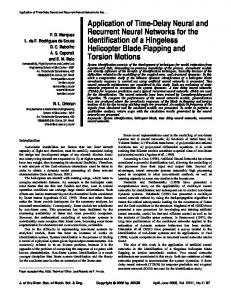
Figure 3. Pole-balancing controller and its internal state. A. The network had three hidden units, which were fed back as the context input with a single step delay to implement a recurrent architecture. The network had eight inputs (see Fig. 2). The two output units represents the force to be applied to the cart in the x and the y direction respectively. B. The activation level of hidden units can be seen as the internal state of the controller agent. This can be plotted as a trajectory in three-dimensional space (see C). Adapted from [22].
over time. The predictability of each neuron was quantified by a supervised learning method which forecasts the next activation value based on the past activation values in the hidden units. The details of the supervised predictor will be discussed in the following section. Note that any reasonable predictor can be used for this, e.g. Hidden-Markov models, and the particular choice is orthogonal to the main argument of this paper. E. Time-series Prediction A sequence of the activation values of a neuron is a time series. The measurements of the activation values take place at a successive and regular time interval [24]. Two-DOF pole-balancing controllers have internal system dynamics that is a function of the current state vector x(t) since the state changes over time. Consequently, the activation level of hidden neurons in the neural network can be considered as a time series. In our case, three sets of time series exist since there are three neurons in the hidden layer of our neural network. Let us assume that we predict value x at time t + 1 which is the very next state from the present. If we can look back N time steps including the current one from time t, we can say that forecasting x(t + 1) means finding a function f (·) using a time series {x(t), x(t − 1), x(t − 2), · · · x(t − N + 1)}): x ˆ(t + 1) = f (x(t), x(t − 1), x(t − 2), · · · , x(t − N + 1)) . Feed-forward neural networks have been widely used to forecast a value given a time series dataset [24]. Fig. 5 gives the basic architecture of a feed-forward neural network
(b) Low internal state predictability
Figure 4. Two controllers with the same level of performance can have very different internal state dynamics. Adapted from [23].
predictor: the predictor (right) and activation patterns (left) explains how they are associated with each other. Note that this predictor is used only to quantify the predictability and is not at all involved in training the cart controller. t+1
t
t−1 t−2 t−3
Figure 5. Measuring predictability in the internal state trajectory. N past data points are applied to the predictor (right) to predict the target point. After training a network, we tested the time-series predictor with a test data set . and measured the accuracy of the prediction. Adapted from [22]
III. EXPERIMENTS AND RESULTS Approximately 150 neural network controllers were successfully trained for the two-DOF pole-balancing task. Successful pole-balancing agents may have a wide variety of internal state dynamics. We grouped those highperformance individuals into high- and low- ISP groups.
More details are illustrated in Fig. 6. Two groups of pole balancers have virtually the same performance in training sessions when it comes to balancing the pole. These steps are summarized as follows: 1) High performance individuals are collected from successfully trained pole-balancers. 2) The internal predictability of each selected individual is measured. 3) Based on the predictability, separate the high performance individuals into two groups: high ISP and low ISP group. 4) The high and low groups are subsequently tested in gradually tougher conditions and under delay in signal transmission. Specifically, we extended our previous work [3] with more conditions that have gradually more difficult levels. We put the agents from the two ISP groups into four different delay conditions where neural signals arrive to the network with a delay of 10ms, 20ms, 30ms, or 40ms. Our results show that the pole-balancers from the high ISP group have a performance edge when coping with delayed signal. All Controllers High−perform. Controllers te al sta intern is s ly a an
High ISP
evolutionary selection process
inter n analy al state sis
Low ISP Figure 6. Overview of the method. Evolved high performance controllers are divided into two groups, high and low ISP groups, based on their internal state predictability values. Adapted from [22].
A. Training the Controllers We previously proposed a pole-balancing agent with recurrent neural networks modulated by NDPIA [3]. The configuration of a controller network was as follows: eleven input nodes (eight input from the simulated physical environment and three context input from the hidden layer), one hidden layer with three neurons, and two output neurons. The eight input values consist of the x and y coordinate in the plane indicating the current cart position, the velocity of the moving cart (x, ˙ y), ˙ the projected angle of the pole from the vertical in the x and the y direction (θx , θy ), and their angular velocity (θ˙x , θ˙y ). These eight parameters describing the current state of the cart were used as the input values. Three context units were fed back to input from the hidden layer of the neural network. Two values from the output neurons, Fx and Fy , represent the force in the x and the y direction. The fourth-order Runge-Kutta method was used to simulate the real world physics [15]. The neural networks were trained by genetic algorithm. The
chromosome encoded the connection weights. Crossover occurred with probability 0.7 and the chromosome was mutated by ±0.3 perturbation rate with probability 0.2. Force between −10N and 10N was applied to the moving cart at regular time intervals (10ms). Note that N is Newton, the unit of force. The pole was 0.5m long and was initially tilted by 0.573◦ (0.01 radian) on the x-z plane and the y-z plane respectively. The area where the cart moved around was 3m × 3m. The fitness value for the genetic algorithm was the number of balancing time steps. In order to count as a success, the neural network must keep the pole within ±15◦ from the vertical for 5,000 steps while maintaining the cart within the area. The number of networks in a population was 50 for an evolutionary epoch. B. Training the Neural Network Predictors The next step is measuring ISP of the successful polebalancers. See Sec. II-E for more details. The size of the sliding window, which is the number of the previous states, was four. The activation values of neurons in the hidden layer formed the input of the neural network predictor. We used 3,000 activation values as training data for each input, and a test set used the next 1,000 steps (3,001 to 4,000). Time series from 1 to 1,000 steps and from 4,001 to 5,000 steps were not used because we did not want to use the somewhat chaotic initial movements and finalized stable movements. The back-propagation algorithm was used to train the predictors with learning rate 0.2. During the test sessions, we compared the predicted value with the real activation value. We chose 10% threshold error rate to calculate the adaptive minimum error threshold when comparing the forecasted activation with the real activation value. The adaptive error rate was determined empirically, based on the performance of the time series predictor. More details can be found in [3]. C. Performance Measurement in High- vs. Low-ISP Groups Two separate experiments were conducted to show validity of our hypotheses. First, we tested and compared the performance of two ISP groups under several different initial conditions that have gradually more difficult levels. See [3] for detail about the previous experimental settings. During training, all the pole-balancers were evolved with the same initial condition where both pole angles were 0.01 radian. During the test sessions, we had those trained agents balance the pole in four conditions in which we gradually increased the level of difficulty: Initial pole angles were (0.04, 0.03), (0.07, 0.04), (0.09, 0.07), and (0.14, 0.08) radian in the test case one, two, three, and four, respectively. Fig. 7 illustrates the performance of the ten pole-balancers from the two ISP groups. The controller IDs were not sorted so the same controller number means the same agent throughout the four test cases.
Low ISP
High ISP Balancing Time (10ms)
4000 3000 2000 1000
High ISP
5000 4000
3000
ISP group and the low ISP group were 98.55%(σ = 1.77%) and 14.47%(σ = 3.88%) respectively. Fig. 9 (b) shows the predictability of the high and the low ISP group.
2000
100
1000
80
0
0 1
2
3
4
5
6
7
8
1
9 10
2
3
4
5
6
7
8
9 10
ISP (%)
Balancing Time (10ms)
Low ISP 5000
Controllers (unsorted)
Controllers (unsorted)
(a) Test Case 1
(b) Test Case 2
Low ISP
Low ISP
60 40
5000
Balancing Time (10ms)
4000 3000 2000 1000
High ISP
5000
0 1
4000 3000
3
1000
4
5
6
7
8
2
3
4
5
6
7
8
High ISP
80
9 10
Controllers (unsorted)
(c) Test Case 3
Low ISP
100 1
9 10
Controllers (unsorted)
151
(a)
0
2
101
2000
0
1
51
Evolved controllers (Sorted)
ISP (%)
Balancing Time (10ms)
20 High ISP
(d) Test Case 4
60 40 20
Figure 7. Novel task performance in high vs. low ISP groups in the initial pole angles (a) 0.04 and 0.03 (b) 0.07 and 0.04 (c) 0.09 and 0.07 (d) 0.14 and 0.08. Each controller (with low vs. high ISP results) corresponds to an experiment run with identical initial condition, so the pairing is meaningful.
0 1
2
3
4
5
6
7
8
9
10
Test cases (unsorted)
(b)
Low ISP High ISP
4000 3000 2000
1000 0 Test 1
Test 2
Test 3
Test 4
Test Cases
Figure 8. Overall performance of two groups in the test cases. The initial pole angles were (0.04, 0.03), (0.07, 0.04), (0.09, 0.07), and (0.14, 0.08) for the test case 1, 2, 3, and 4 respectively. All angles are represented in radian. There is no significant different between low ISP and high ISP group when the initial condition is not much more difficult than the training condition. However, it becomes clear that the controllers in the high ISP group perform better than those in the low ISP group as the initial conditions become harder.
The second experiment was to test how the internal state of an agent affects its performance under conditions where input signals are delayed. Again we prepared ten high ISP pole-balancers and ten low ISP ones. Note that we avoided few extremes in both the lowest and the highest ISPs. The criterion of high or low predictability is that all three neurons from the hidden layer have high or low predictable internal state trajectories. The average prediction rates in the high
4500 4000 3500 3000 2500 2000 1500 1000 500 0
High ISP Low ISP
0
1
2
3
4
Number of Controllers
5000
Then we applied input with different levels of delay to the neural network controllers. Our results demonstrate that the high ISP group has better performance, effectively handling delayed signals (Fig. 10). Balancing Duration (10ms)
Balancing Time (10ms)
Our results show that the performance differences between two groups were even greater as the difficulty of the task increases. Fig. 8 shows the overall performance of the two groups in all four test cases. The performances of agents in the high ISP group showed slow decrease while those in the low ISP group quite decrease as the difficulty increases.
Figure 9. (a) Sorted predictability of successful pole-balancing controllers during training. (b) Comparison of the average predictability from two ISP groups: high and low ISP. Agents with the top 10 and the bottom 10 internal state predictability from (a) are shown here. Note that few extremes from both sides are eliminated. Each data point means an average prediction rate of three hidden neurons of each agent. Error bars indicate standard deviation.
9 8 7 6 5 4 3 2 1 0
High ISP Low ISP
0
Delay (10ms)
(a)
1
2
3
4
Delay (10ms)
(b)
Figure 10. Effect of delay on the high- and the low-ISP group. Performances of pole-balancers under delayed signal conditions are shown. (a) The difference in pole balancing time between the two groups. (b) The number of controllers that can balance the pole under each delay condition.
IV. CONCLUSIONS The main contribution of our work is that we showed that internal neural dynamics not only affect performance of the neural network controllers but also help them cope with longer signal transmission delay. These results suggest that internal properties of an agent have a survival value
and that the agents whose internal neural dynamics is more predictable have a performance edge when they faced with delayed signals. The implication of these findings is that predictive neural dynamics in internal state trajectories of an agent may serve as a delay compensation mechanism. This is important since predictability of internal state may lead to an ability to predict. Future directions include extending our work to other more complex tasks.
[14] C. W. Anderson, “Learning to control an inverted pendulum using neural networks,” IEEE Control Systems Magazine, vol. 9, pp. 31–37, 1989. [15] F. Gomez and R. Miikkulainen, “2-D pole balancing with recurrent evolutionary networks,” in Proceeding of the International Conference on Artificial Neural Networks (ICANN), Sk¨ovde, Sweden, Sep. 1998, pp. 758–763.
R EFERENCES
[16] E. S. Fortune and G. J. Rose, “Short-term synaptic plasticity as a temporal filter,” Trends in Neurosciences, vol. 24, pp. 381–385, 2001.
[1] R. Nijhawan, “Visual prediction: Psychophysics and neurophysiology of compensation for time delays,” BEHAVIORAL AND BRAIN SCIENCES, vol. 31, pp. 179–239, 2008.
[17] H. Markram, Elementary principles of nonlinear synaptic transmission. London, UK: Springer-Verlag, 2003.
[2] S. J. Thorpe and M. Fabre-Thorpe, “Seeking categories in the brain,” Science, vol. 291, pp. 260–263, 2001. [3] J. Kwon and Y. Choe, “Enhanced facilitatory neuronal dynamics for delay compensation,” IJCNN 2007. International Joint Conference on Neural Networks, 2007, pp. 2040–2045, 2007. [4] K. L. Downing, “The predictive basis of situated and embodied artificial intelligence,” in GECCO ’05: Proceedings of the 2005 conference on Genetic and evolutionary computation. New York, NY, USA: ACM Press, 2005, pp. 43–50. [5] R. R. Llin´as, I of the Vortex. 2001.
[18] H. Lim, “Facilitatory neural dynamics for predictive extrapolation,” Ph.D. dissertation, Texas A&M University, 2006. [19] H. Lim and Y. Choe, “Facilitatory neural activity compensating for neural delays as a potential cause of the flash-lag effect,” in Proceedings of the International Joint Conference on Neural Networks (IJCNN), Montreal, QC, Canada, Aug. 2005, pp. 268–273. [20] F. Gomez and R. Miikkulainen, “Solving non-markovian control tasks with neuroevolution,” in Proceedings of the International Joint Conference on Artificial Intelligence (IJCAI), T. Dean, Ed. San Francisco, CA: Morgan Kaufmann, 1999, pp. 1356–1361.
Cambridge, MA: MIT Press,
[6] B. Krekelberg and M. Lappe, “A model of the perceived relative positions of moving objects based upon a slow averaging process,” Vision Research, vol. 40, pp. 201–215, 2000. [7] ——, “Neural latencies and the position of moving objects,” Trends Neurosciences, vol. 24, pp. 335–339, 2001. [8] B. Krekelberg, “Sound and vision,” Trends in Cognitive Sciences, vol. 7, pp. 277–279, 2003. [9] H. Lim and Y. Choe, “Compensating for neural transmission delays using extrapolatory neural activation in evolutionary neural networks,” Neural Information Processing–Letters and Reviews, vol. 10, pp. 147–161, 2006. [10] J. Liaw and T. W. Berger, “Dynamic synapse: Harnessing the computing power of synaptic dynamics,” Neurocomputing, vol. 26-27, pp. 199–206, 1999. [11] R. c. M. Daniel M. Wolpert and M. Kawato, “Internal models in the cerebellum,” Trends in cognitive science, vol. 2, pp. 338–347, 1998. [12] E. T. Rolls, “A computational neuroscience approach to consciousness,” Neural Networks, vol. 20, no. 9, pp. 962– 982, 2007. [13] V. Itskov and C. Curto, “From spikes to space: reconstructing features of the environment from spikes alone,” BMC Neuroscience, vol. 8, no. Suppl 2, p. P158, 2007.
[21] ——, “Active guidance for a finless rocket through neuroevolution,” in Proceedings of the Genetic and Evolutionary Computation Conference (GECCO), Chicago, IL, Jul. 2003, pp. 2084–2095. [22] J. R. Chung, J. Kwon, and Y. Choe, “Evolution of recollection and prediction in neural networks,” in In Proceedings of the International Joint Conference on Neural Networks. IEEE Press, 2009, pp. 571–577. [23] J. Kwon and Y. Choe, “Internal state predictability as an evolutionary precursor of self-awareness and agency,” in ICDL 2008. Proceedings of the seventh international conference on development and learning, IEEE, 2008, pp. 109–114. [24] R. J. Frank, N. Davey, and S. P. Hunt, “Time series prediction and neural networks,” J. Intell. Robotics Syst., vol. 31, no. 1-3, pp. 91–103, 2001.