Algorithmica (1998) 22: 250–274
Algorithmica ©
1998 Springer-Verlag New York Inc.
Semidynamic Algorithms for Maintaining Single-Source Shortest Path Trees1 D. Frigioni,2,3 A. Marchetti-Spaccamela,3 and U. Nanni3,4 Abstract. We consider the problem of updating a single-source shortest path tree in either a directed or an undirected graph, with positive real edge weights. Our algorithms for the incremental problem (handling edge insertions and cost decrements) work for any graph; they have optimal space requirements and query time, but their performances depend on the class of the considered graph. The cost of updates is computed in terms of amortized complexity and depends on the size of the output modifications. In the case of graphs with bounded genus (including planar graphs), graphs with bounded arboricity (including bounded degree graphs), and graphs with bounded treewidth, the incremental algorithms require O(log n) amortized time per vertex update, where a vertex is considered updated if it reduces its distance from the source. For general graphs √ with n vertices and m edges our incremental solution requires O( m log n) amortized time per vertex update. We also consider the decremental problem for planar graphs, providing algorithms and data structures with analogous performances. The algorithms, based on Dijkstra’s technique [6], require simple data structures that are really suitable for a practical and straightforward implementation. Key Words. Single-source shortest path, Dynamic algorithms, Amortized complexity, Output complexity.
1. Introduction. Finding shortest paths is a fundamental and well-studied problem in computer science, and its solution in many situations may provide answers to other interesting problems, especially in planar graphs, such as maximum flow and transportation problems. The best off-line solution for the single-source shortest path problem on general graphs G = (V, E) with positive real edge weights is the implementation of Dijkstra’s algorithm by using Fibonacci heaps [10], that runs in O(m + n log n) time, where n = |V | and m = |E|. If we consider planar √ graphs, then a classical solution is due to Frederickson [9], with a running time of O(n log n) in a graph with n vertices. Recently Frederickson’s approach, based on decomposition of graphs by using Lipton and Tarjan’s separator theorem [15], has been extended by Klein et al. [13] to get an optimal O(n) time algorithm to find a single-source shortest path tree in a planar graph with nonnegative edge lengths.
1 This work was partially supported by EC ESPRIT Long Term Research Project ALCOM-IT under Contract No. 20244, and by PROGETTO FINALIZZATO TRASPORTI 2 of the Italian National Research Council (CNR). 2 Dipartimento di Matematica Pura ed Applicata, Universit` a di L’Aquila, via Vetoio, I-67010 Coppito (AQ), Italy.
[email protected]. 3 Dipartimento di Informatica e Sistemistica, Universit` a di Roma “La Sapienza”, Via Salaria 113, 00198 Roma, Italy. {alberto,nanni}@dis.uniroma1.it. 4 Part of this work was developed while this author was visiting the International Computer Science Institute, 1947 Center Street, Berkeley, CA 94704, USA.
Received January 1995; revised February 1997. Communicated by D. Eppstein.
Semidynamic Algorithms for Maintaining Single-Source Shortest Path Trees
251
The dynamic version of a shortest path problem consists in dealing with updates on the structure of the graph, while maintaining the possibility of answering queries on shortest paths without recomputing them from scratch. Various approaches have been considered in literature to deal with dynamic shortest path problems both for single-source and all-pairs versions [4], [7], [8], [13], [14], [19], [20], providing several noncomparable solutions, each characterized by a given setting for (a) the kind of considered graph and edge weights, (b) the set of allowed updates on the structure of the graph, and (c) the adopted measure of performances. Some of the proposed solutions pursue a tradeoff between query and update time, while others carry out an explicit update of shortest paths information when modifications occur to get optimal query time. The former approach aims at the target of reducing the worst-case time of interleaved queries and updates; the latter is mandatory in situations where restoring shortest paths information is explicitly required and it may be preferred if the target is to optimize the amortized time. Fully dynamic solutions (where both insertions and deletions of edges are allowed) have been devised by considering a query/update tradeoff only for planar graphs. In the case of unrestricted edge weights, Klein et al. [13] propose a fully dynamic solution to maintain all-pairs shortest paths requiring O(n 9/7 log D) time both for queries and updates, where D is the sum of all the edge weights. A sublinear approximation scheme for the fully dynamic single-source problem in planar graphs has been proposed in [14]. These solutions use a topological partition of the graph based on a recursive application of the planar separator theorem [15]: all these algorithms are complex and far from being practical. The explicit update of all-pairs shortest paths for general graphs has been considered, for example, in [4], [7], and [20]. In the particular case of edge insertions in a directed graph G = (V, E), with |V | = n and |E| = m, and integer edge weights in the range [0..C], an algorithm is provided in [4] requiring O(Cn log n) amortized time per edge insertion in any sequence of Ä(m) insertions, while queries may be answered in constant time. We remark that, in the case that explicit updates are required and real values for edge weights are allowed, no efficient dynamic solution may exist for this problem in both the standard worst-case and amortized cost models. Output Complexity. In several applications, such as incremental compilation, dataflow analysis, and graphical and/or interactive applications where the user is expected to see any change, explicit updates must be carried out after an input modification is specified. In these situations a different measure of performance may be considered, besides the classical worst-case and amortized analysis [21]. Ramalingam and Reps in [18] and [19] propose measuring the cost of a dynamic algorithm in terms of output complexity; a similar notion was also used by other authors (see, e.g., [2]). An input modification µ is defined as a set of edge operations (insertions, deletions, or cost updates), transforming a graph G = (V, E) to a new graph G 0 = (V, E 0 ). In the case of a single-source shortest path problem with source s, the set of vertices Affected(G, µ) are those that have a different distance from s in G and G 0 . Hence any algorithm which explicitly updates output information cannot have a cost smaller than the number of affected vertices. Here we extend this notion to sequences of input modifications. We consider a graph
252
D. Frigioni, A. Marchetti-Spaccamela, and U. Nanni
G and a sequence σ = hµ1 , µ2 , . . . , µq i of input modifications. Each input modification µi ∈ σ consists of a set of edge operations to be performed on graph G i−1 , with G 0 ≡ G, and gives the new graph G i . We denote this situation by writing µ1
µq
µ2
G 0 −→ G 1 −→ G 2 · · · G q−1 −→ G q . After each input modification µi ∈ σ is specified we are required to update the current output information: in the case of a single-source shortest path problem, the output information consists of the value of distances from the source s for any vertex x ∈ V . Let δi be the set of output updates, i.e., the set of vertices changing their distance from source s due to input change µi (hence |δi | = |Affected(G i−1 , µi )|). The number of output updates in a sequence σ is the sum of the number of output updates for any input modification in the sequence: X |δi |. |1(σ )| = µi ∈σ
If A G (σ ) is the time required by a generic algorithm A to handle a sequence σ , we say that algorithm A requires α amortized time per vertex update if, for any sequence σ , the following inequality holds: A G (σ ) ≤ α · |1(σ )| + |σ | + constant. No algorithm can process sequence σ performing explicit updates in less than |1(σ )| + |σ | time: this is the time spent by an ideal algorithm that updates useful output information with no additional cost, i.e., requiring constant time per output modification. Achieved Results. We consider the semidynamic single-source shortest path problem for both directed and undirected graphs with real positive edge weights, providing algorithms that are both practical and efficient. Ramalingam and Reps first studied this problem in terms of output complexity. In [19] they provided a fully dynamic algorithm for general graphs. In particular they consider an extended size of the set of vertices that modify their distance, defined as follows: kδk = kAffectedk is the sum of the number of affected vertices plus the number of edges having at least one affected endpoint, due to the input change δ. Using such a parameter, they obtain a solution such that the cost of updating the output data structures due to a set δ of edge deletions and edge insertions is O(kδk · log kδk). In this paper we separately consider the incremental problem (in which any input modification µi contains only insert and weight decrease operations on the edges) and the decremental problem (with allowed delete and weight increase operations). We provide algorithms and data structures for the incremental problem working for any graph. Space requirements are optimal, that is, O(m + n) for a graph with n vertices and m edges, as well as query time, that is O(1) to get the distance between the source and any other vertex, and O(l) to provide a shortest path with l edges. Our algorithms for the decremental problem work only for planar graphs, and have analogous performances. In both cases, building our data structures from scratch for any graph G = (V, E), with n = |V | and m = |E|, requires total time O(m + n log n). In order to study the output complexity of the incremental algorithm, we provide a characterization of a graph according to the existence of a k-bounded accounting
Semidynamic Algorithms for Maintaining Single-Source Shortest Path Trees
253
function. An accounting function A is a function that for each edge (x, y) determines either vertex x or vertex y as the owner of that edge; A is a k-bounded accounting function for G if k is the maximum over all vertices x of the cardinality of the set of edges owned by x. An analogous notion has been previously introduced in [5], where the authors define an orientation of a graph G = (V, E) as a function ω which replaces each edge (x, y) ∈ E by a directed edge x → y or y → x. If degω+ (x) is the out-degree of vertex x under the orientation ω, then ω is k-bounded if, for each vertex x ∈ V , degω+ (x) ≤ k. In particular they prove that each planar graph has a five-bounded acyclic orientation that can be found in linear time. Furthermore they prove the existence of a three-bounded orientation for each planar graph and provide a linear time algorithm for finding such orientation. The existence of the same three-bounded orientation has been shown in [17] by using the property that arboricity a(G) of a planar graph G satisfies a(G) ≤ 3, but in that case the corresponding algorithm requires more than linear time. Clearly the notions of k-bounded orientation and k-bounded accounting function for an undirected graph G coincide. Since we deal with directed and undirected graphs, for the sake of clarity in what follows we adopt the terminology of the accounting function. The above defined parameter k can be bounded in different ways by using structural properties of the graph. For example, k is immediately bounded by the maximum degree of G. Furthermore, it is easy to see that the value of parameter k for any graph G is bounded by the arboricity of G and by the treewidth of G. Moreover, it is possible to √ show that k = O(1 + γ ), where γ is the genus of G, by observing that the pagenumber √ of a genus γ graph is O( γ ) [16]; since the genus of a graph √ is always less than its number of edges, it follows that a graph with m edges has a O( m)-bounded accounting function. For any incremental sequence, our algorithm requires O(k log n) amortized time per vertex update. Our solution is within a logarithmic factor far away from an optimal solution with explicit updates. For the mentioned classes of graphs and updates (note that Ramalingam and Reps’ solution is fully dynamic), our results improve the time bounds given in [18] and [19], expressed in terms of parameter kδk. In fact, |δ| ≤ kδk ≤ n · |δ|; furthermore, there are cases in which the upper bound is tight. In the particular case of a planar graph, the optimal off-line solution by Klein et al. [13] (requiring O(n) time) may be better than our dynamic algorithm if a large part of the solution has to be updated. On the other side, the motivation behind the solution proposed in this paper is to avoid high computational costs for small changes, and to obtain practical algorithms. The results are obtained by introducing a new technique based on storing at each vertex q, for each neighbor z, information concerning a shortest path from source s that uses edge (q, z). This information is used during the edge updates in the following way: after an edge insertion (or weight decrease), a vertex q that decreases its distance from s can detect which neighbors may improve their distance from s; during edge deletions (or weight increases), a vertex q which looses its current best neighbor connecting to s can select the best alternative among the remaining neighbors. The basic idea is that a vertex q that changes its distance from the source can avoid testing all the neighbors, but only test the right ones: this can be done by performing lazy updates. The strategy that is pursued by our algorithms can be summarized as follows: in the incremental
254
D. Frigioni, A. Marchetti-Spaccamela, and U. Nanni
problem, a vertex that improves (i.e., decreases) its distance from the source must send updates only to neighbors that in turn improve their distance from the source; in the decremental problem a vertex that loses its connection to the source, must know the best alternative neighbor to replace the connection. Since the information about the new value of distances from the source are broadcasted only to the interested neighbors, a deferred update regarding a neighbor may occur as soon it is strictly required. The paper is organized as follow. After the preliminaries, in Section 3 we introduce our algorithm for the incremental single-source shortest path problem, limiting our attention to input modifications consisting of single edge insertions. In Section 4 we extend the result to the batch incremental problem, where each modification consists of a set of edge operations. In Section 5 we show the decremental algorithm for planar graphs. Some concluding remarks are provided in Section 6.
2. Preliminaries. The problem we deal with is to maintain a single-source shortest path tree from a given source vertex s for a weighted (directed or undirected) graph, while performing a sequence of query and modification operations of the following kinds: (a) (b) (c) (d) (e) (f)
distance(x): report the current distance between source s and vertex x; path(x): report a minimum cost path between source s and vertex x; insert(x, y, w): insert edge (x, y) with weight w; delete(x, y): delete edge (x, y); increase(x, y, ε) (weight increase): increase by quantity ε the weight of edge (x, y); decrease(x, y, ε) (weight decrease): decrease by quantity ε the weight of edge (x, y).
Our goal is to maintain explicitly distances from s and a single-source shortest path tree with source in s, so that queries (a) and (b) can be answered respectively in constant time and in a time proportional to the edges of the traced minimum path. In this paper we only consider the semidynamic version of the problem. Namely, besides the query operations, we deal with monotonic sequences of either insert and weight decrease operations (denoted as the incremental problem) or delete and weight increase operations (the decremental problem). In the following we assume standard graph theoretical terminology as contained, for example, in [1] and [11]. In particular the genus of a graph G is the smallest integer γ such that it is possible to draw G on a planar (or spherical) surface with γ handles with no edge intersections (see, e.g., [11]); the arboricity a(G) of a graph G is the minimum number of edge-disjoint spanning forests into which G can be decomposed [11]; another related parameter is the treewidth of a graph for which we refer to [3]. Hereafter in this paper we consider a weighted graph G = (V, E), with real positive edge weights defined on the edges, and we denote as wx,y the weight of an edge (x, y). Throughout the paper we distinguish a fixed source vertex s ∈ V , while d(x) denotes the minimum distance between vertex x and source s. A single-source shortest path tree with source s is a tree T (s) ⊆ G such that, for any vertex x ∈ V , T (s) contains a shortest path from s to x in G. T ( j) denotes the subtree of T (s) rooted in j. An edge (x, y) is internal for T ( j) if both x and y are vertices in T ( j). An edge (x, y) is a tree-edge if (x, y) ∈ T (s), otherwise it is a nontree edge. Any vertex x ∈ V has one parent (except for source s) and a (possibly empty) set of children in T (s).
Semidynamic Algorithms for Maintaining Single-Source Shortest Path Trees
255
Let G = (V, E) be a weighted graph with source s, and let (x, y) be an edge to be inserted in (deleted from) G to give the new graph G 0 = (V, E ∪ {(x, y)}) (G 0 = (V, E − {(x, y)})). The distance of a vertex z from the source, the parent of a vertex z, and the new version of single-source shortest path tree in the new graph G 0 are denoted as d 0 (z), parent0 (z), and T 0 (s), respectively. The proofs of all propositions given in the paper are straightforward and therefore they are omitted.
3. The Incremental Problem. An instance of the incremental single-source shortest path tree and distance problem is defined by a weighted graph G = (V, E), a source s ∈ V , a single-source shortest path tree T (s), and by a sequence σ = hµ1 , µ2 , . . . , µq i of input modifications. Any input modification µi ∈ σ is a set of insert and weight decrease operations to be performed on graph G i−1 , with G 0 = G, and gives the new graph G i . After each input modification µi ∈ σ is specified we are required to update the current version Ti−1 (s) of the single-source shortest path tree with source in s, to give the updated version Ti (s). Furthermore, we are required to maintain the mapping defined by function d, i.e., the value d(x) denoting the current distance from source s to vertex x, for any x ∈ V . The number of vertex updates required by an input modification µi , denoted as |δi |, is the number of vertices that in graph G i have a smaller distance from s than in graph G i−1 . Hence the number of vertex updates required by a sequence σ of input modifications applied to graph G is the following: X |δi |. |1(σ )| = µi ∈σ
We prove that, for any incremental sequence σ , our algorithm requires O(|σ | + |1(σ )| · k log n + m + n log n) total time, where k is a parameter that depends on the structure of the graph, n is the number of vertices, and m is the initial number of edges. O(m + n log n) is the initialization time to set up the required data structures, possibly performed during the updates and O(k log n) is the amortized time per output update, where k is bounded as follows: √ for graphs with m edges; k = O( m) √ for graphs with genus γ ; k = O(1 + γ ) k≤3 for planar graphs; k≤a for graphs with arboricity a; k≤d for graphs with maximum degree d; k≤t for graphs with treewidth t. In the following we consider the incremental problem in the particular case that any input change µi has size 1, i.e., consists of a single edge operation. In Section 4 we consider the general problem. A single-source shortest path tree T (s) = (V, E T ) is represented explicitly, maintaining a bipartition of edges in tree and nontree edges. For the sake of clarity we present first a procedure based on Dijkstra’s algorithm that correctly updates T (s) and d, but does not satisfy the claimed bounds. The final algorithm is given in Section 3.1. It is easy to see
256
D. Frigioni, A. Marchetti-Spaccamela, and U. Nanni
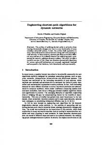
Fig. 1. Pseudocode of procedure Dijkstra Insert.
that after an edge insertion or a weight decrease operation, distances of edges from the source can only decrease; the following proposition gives a simple test to decide whether there is at least one vertex whose distance from the source decreases as a consequence of an insertion or a weight decrease operation. PROPOSITION 3.1. Let G = (V, E) be a graph and let G 0 be the graph obtained from G after the insertion of edge (x, y) or after the decrease of the weight of edge (x, y). Let wx,y be the weight of edge (x, y) in G 0 and, without loss of generality, assume that d(y) > d(x). Then d 0 (y), the distance of y from the source in G 0 , is equal to min{d(y), d(x)+wx,y }. If d(y) = d 0 (y), then there is no vertex q for which d 0 (q) < d(q). The algorithm in Figure 1, based on Dijkstra’s algorithm for finding a single-source shortest path tree, first computes the distance of y from the source in the updated graph. If this distance is unchanged, then the procedure terminates; otherwise a search starting from vertex y is performed; in step 3 a heap is initialized with vertex y with priority equal to d(x) + wx,y ; in step 4 the search is performed. Namely, the following steps are executed in an iteration of the while loop. First the vertex q with minimum priority is deleted from the heap Q, then the distance d(q) of q from the source is set to be equal to the priority of q. Finally, each vertex r that is adjacent to q is examined to determine whether the shortest path from s to r passing through q is shorter than the previous known
Semidynamic Algorithms for Maintaining Single-Source Shortest Path Trees
257
path; in this case, if vertex r is already in Q, then its priority is updated, otherwise vertex r is inserted in Q with priority d(q) + wq,r . It is not difficult to show the correctness of the procedure in Figure 1. However, the running time of the procedure depends on the number of edges that are scanned in line 13. Note that there could be O(n) vertices adjacent to vertex q that do not change their distance from the source in the updated graph; therefore the running time of procedure Dijkstra Insert for the ith update is O(n · |δi | log |δi |) in the worst case, where δi is the set of vertex updates, i.e., the set of vertices changing their distance from source s due to the ith input modification. It is possible to show that the same bound holds also by using amortized analysis. The remainder of this section is devoted to presenting an improved algorithm that, when a vertex z improves its distance from the source, does not broadcast this information to all neighbors, but only to a subset. DEFINITION 3.1. Let G = (V, E) be a weighted graph, and let T (s) be a single-source shortest path tree with source in s. The temperature of edge (q, r ) (of vertex r ) relative to vertex q is tq (r ) = d(r ) − wqr . The following definition allows us to determine those edges that are useful for finding improved distances. DEFINITION 3.2. Let G = (V, E) be a weighted graph with source s and let d(r ) be the distance from source s to vertex r . An edge (q, r ) is hot for q during the insertion or the weight decrease of edge (x, y) if making q the new parent of r would allow us to obtain a path from s to r shorter than the current (old) value of d(r ), i.e., if q would be a better parent for r with respect to the current one. In this case vertex r is hot for q. The following proposition is an immediate consequence of the above definitions. PROPOSITION 3.2. Let G = (V, E) be a graph, let s be a source, and let G 0 be the graph obtained from G after an insert or weight-decrease operation on one edge. Let d(q) and d 0 (q) be the distances of vertex q from s in G and G 0 , respectively. Edge (q, r ) is hot for q during the considered edge update if and only if d 0 (q) < d(r ) − wq,r = tq (r ). In order to reduce the cost of scanning edges in procedure Dijkstra Insert the above proposition might be used to detect hot edges: after a new distance d 0 (q) < d(q) is computed for vertex q, the new distance d 0 (q) is “announced” to a neighbor r only if the edge (q, r ) is hot for q, i.e., the old distance d(r ) from the source to r in G is larger than the length of a path passing through q and using edge (q, r ). The above proposition is not sufficient to obtain the claimed bounds on the running time of Insert, since the detection of hot edges requires maintaining the temperature of edges; this operation could require the scanning of all edges incident to vertex q. To avoid this problem the algorithm of Figure 2 does not maintain the temperature of edges but maintains a priority that is higher or equal to the temperature.
258
D. Frigioni, A. Marchetti-Spaccamela, and U. Nanni
Fig. 2. Pseudocode of procedure Insert.
3.1. An Incremental Algorithm for Shortest Paths. The data structures to be maintained, while performing edge updates to the graph G = (V, E), are the following. For each vertex q, the adjacency list of neighbors is maintained as a back-heap B(q), which is a max-based priority queue of the vertices (of the edges) leaving q. The priority of edge (q, r ) (of vertex r ) in B(q) is denoted as pq (r ); for any updated vertex q, an edge (q, r ) is possibly hot if d 0 (q) < pq (r ). We will see (Lemma 3.1) that for any edge (q, r ) we have pq (r ) ≥ tq (r ); therefore a hot edge is also a possibly hot edge. The algorithm is given in Figure 2. It differs from the procedure of Figure 1 in step 4 and it has in addition step 5; in step 4 procedure Insert performs a search that is similar to the search done by procedure Dijkstra Insert. The main difference is that when vertex q is deleted from the global heap Q the algorithm considers only a subset of its neighbors. In particular, a neighbor r of q is considered only if priority
Semidynamic Algorithms for Maintaining Single-Source Shortest Path Trees
259
pq (r ) is greater than d 0 (q); for any such vertex r , which might be hot or not, the actual temperature tq (r ) is computed and the priority of r in B(q) is set to tq (r ). This allows us to know whether vertex q is actually hot for r ; in this case the priority of vertex r in Q is updated if r is already in Q, otherwise r is inserted in Q. In step 5 for each hot edge (x, y) the priorities px (y) and p y (x) are updated to the values tx (y) and t y (x), respectively, in order to guarantee that each hot vertex holds updated priorities for its hot neighbors. These updates cannot be performed in the previous step each time that a hot edge is detected, because at that time one of the two endpoints of the edge could not know its actual shortest distance from the source s. Note that if a neighbor r of q is not possibly hot for q, it will not announce the new temperature of vertex q, and the update of the priority will be deferred until either r becomes possibly hot for q, or vice versa: this is called a lazy update. LEMMA 3.1. Let G = (V, E) be a graph and let G 0 be the new graph after an insertion or weight decrease of edge (x, y). After the execution of procedure Insert for any edge (q, r ) we have that pq (r ) ≥ tq (r ). PROOF. When edge (q, r ) is initially inserted in the graph, then the initial value of the priority pq (r ) coincides with the temperature tq (r ). Assume that the condition is true before the insertion or weight decrease of edge (x, y); we show that it is true after the execution of the procedure Insert. If (x, y) 6= (q, r ), then observe that the temperature tq (r ) cannot increase as a consequence of the modification. There are two possibilities: if the priority pq (r ) is not modified by the procedure, then pq (r ) ≥ tq (r ) must be true after the execution of the procedure Insert; on the other hard, if the priority pq (r ) is modified, then it is set to be equal to the temperature tq (r ). If (x, y) = (q, r ), then the temperature tq (r ) can increase as a consequence of a weight decrease operation on edge (x, y); however, in this case the algorithm in step 1 computes temperatures tq (r ) and tr (q) and updates the corresponding priorities in B(q) and B(r ). The lemma implies that the priority of an edge is never less than the corresponding temperature, and therefore the set of hot vertices for q is always included in the set of possibly hot vertices. Hence, considering all vertices in heap B(q) whose priority is above the threshold value d 0 (q), allows us to detect all the neighbors that are actually hot for q. LEMMA 3.2. Let G = (V, E) be a graph and let G 0 be the new graph after the insertion or weight decrease of edge (x, y). Procedure Insert correctly computes the distances from the source. PROOF. Suppose that all distances have been correctly computed before the update operation on edge (x, y) is performed and that after the execution of procedure insert on edge (x, y) the algorithm is not correct. Then there must exist two vertices v and z such that: (i) the value D found by the algorithm as the distance from the source to z is
260
D. Frigioni, A. Marchetti-Spaccamela, and U. Nanni
not correct; (ii) the algorithm correctly computes the distance from the source to v; (iii) edge (v, z) is in the shortest path tree after the update operation. Conditions (i)–(iii) above imply the following inequalities: d 0 (v) + wv,z = d 0 (z) < D ≤ d(z). There are two possibilities depending on the new distance of vertex v. (1) d(v) = d 0 (v). In this case we have that d 0 (z) = d 0 (v) + wv,z = d(v) + wv,z ≥ d(z). Since d 0 (z) ≤ d(z) it follows that d 0 (z) = d(z). This contradicts the fact that distances have been correctly computed before the considered update operation. (2) d(v) > d 0 (v). It is sufficient to show that the algorithm updates the priority of vertex z in the global heap Q to the value d 0 (v)+wv,z . If (x, y) = (v, z), then this operation is performed in step 3. If x = v and z 6= y, then by (iii) above (x, z) is in the shortest path tree after the update operation; since (x, y) is in the updated shortest path tree it follows that d 0 (z) = d(z) contradicting the fact that distances have been correctly computed before the considered update operation. If x 6= v we consider the behavior of the algorithm immediately after the step that computes the distance d 0 (v) of vertex v from the source in the updated graph G 0 . The algorithm considers all vertices r in the heap B(v) such that pv (r ) > d 0 (v). Since d 0 (v) < d(z) − wv,z by Lemma 3.1 vertex z is considered, edge (v, z) is scanned and the priority of z in Q is set to be d 0 (v) + wv,z . This contradicts the fact that the distance of z from the source is not correctly computed. Building the required data structures from scratch takes O(m + n log n) time for any graph G = (V, E), with n vertices and m edges. We now show that the number of operations required by algorithm Insert shown in Figure 2 (namely, the number of possibly hot edges which are scanned) while performing a sequence σ of insert and weight decrease operations is bounded by a function of the quantity |1(σ )|. DEFINITION 3.3. Let G = (V, E) be a (directed or undirected) graph. An accounting function for G is any function A: E → V such that, for any edge (x, y) ∈ E, A(x, y) is either x or y, which is called the owner of edge (x, y). Furthermore, A: E → V is a k-bounded accounting function for G if, for any vertex x ∈ V , the set A−1 (x) = {(x, y) | A(x, y) = x} of the edges owned by x has cardinality at most k. The next theorem characterizes the amortized complexity of algorithm Insert with respect to the notion of a k-bounded accounting function. In a context where edges are incrementally inserted, we consider a k-bounded accounting function to refer to the final graph (i.e., after that all the insertions took place). Note that such a notion is a monotone property of the graph. In other words, if G has a k-bounded accounting function, then any subgraph G 0 ⊆ G has the same property. THEOREM 3.3. Let G = (V, E) be a (directed or undirected) graph, let s be a distinguished vertex in V , and let T (s) be a single-source shortest path tree. Let σ be a sequence of insert and weight decrease operations to be performed on G requiring |1(σ )| vertex updates. If there exists a k-bounded accounting function for G, then it is possible to update T (s) and distances of all vertices from s during the sequence σ of operations in total time O(k |1(σ )| log n + |σ |), where n = |V |. The space bound is
Semidynamic Algorithms for Maintaining Single-Source Shortest Path Trees
261
O(|V | + |E|), while queries may be answered in optimal time: O(1) to report a distance of any vertex from the source, and O(l) to trace a minimum cost path with l edges. PROOF. The correctness proof is given in Lemma 3.2. As far as the space bound is concerned, we observe that, besides the basic representation for graph G, the tree T (s), and the mapping that defines distance function d, the additional structures consist of a priority queue B(z) of incident edges for any vertex z. The total number of items in such queues is 2|E|. Queries about the distance from the source are answered in constant time since they are explicitly stored, and an optimal path from s to any other vertex can be traced by using the tree T (s) in time proportional to the number of edges in the reported path. Any heap operation performed by the algorithm requires O(log n) time; therefore it is sufficient to prove a O(k |1(σ )|) bound on the number of times that the condition pq (r ) > d(q) of the innermost loop (lines 13–24) is checked in an incremental sequence of edge operations. We prove the claim by using a credit argument. Our credit policy is the following: (1) at the beginning each vertex q is given 2k +1 credits (two credits for any edge owned by q and one credit for the vertex itself); (2) as soon as a vertex q decreases its distance from source s, it is given 2k + 1 credits (discarding any residual credit); (3) each time the condition pq (r ) > d(q) of the innermost loop is checked (lines 13–24), one credit is paid. If the condition is not verified, vertex q will pay; if the condition is satisfied and an edge is scanned, the owner of the edge is charged for the cost. In order to show that the credits balance at any vertex will never become negative suppose that q is the owner of edge (q, r ); we show that edge (q, r ) can be scanned at most twice between any two consecutive updates of distance d(q). As soon as q is updated (improving its distance from source s), for any edge (q, r ) leaving q, one of two possible cases may arise: 1. Edge (q, r ) is scanned. After this scan the priority of q in B(r ) is equal to the actual temperature of the edge (see step 5 in procedure Insert). It is sufficient to show that there could be at most one scan of edge (r, q) starting from vertex r before the following update of d(q). In fact after the first scanning (r, q) starting from vertex r is performed, q will actually be hot for q and the distance of q from the source is decreased. 2. Edge (q, r ) is not scanned. In this case the priority pr (q) might be greater than the corresponding temperature tr (q). Therefore when the algorithm updates d(r ) and edge (q, r ) is scanned from r for the first time, no shorter path from the source to q will be found; however, after that pr (q) = tr (q) (the priority is equal to the temperature). Hence when the second scanning of edge (r, q) starting from vertex r is performed, q will actually be hot for r and the distance of q from the source is decreased. The following corollaries characterize the time bound of our algorithm for some known classes of graphs.
262
D. Frigioni, A. Marchetti-Spaccamela, and U. Nanni
COROLLARY 3.4. The incremental single-source shortest path problem can be solved in O(k log n) amortized time per output update, where, for any graph G = (V, E): √ (1) k = O(1 + γ ) if G has genus γ (hence k = O(1) if G is planar); (2) k ≤ a if G has arboricity a; (3) k ≤ d if G has maximum degree d; (4) k ≤ t if G has treewidth t. PROOF. If graph G belongs to one of the listed classes of graphs, then the proof trivially holds as a consequence of the following observations: √ 1. In case (1), since a graph G with genus γ has pagenumber O( γ ) [16], and the √ arboricity of a planar graph is less equal than three [17], then there exists a γ bounded accounting function for G. 2. As far as cases (2)–(4) are concerned it is easy to show that the class of graphs with bounded arboricity includes graphs with bounded degree and graphs with bounded treewidth. Furthermore, it is trivial to define a k-bounded accounting function for a graph with arboricity k. COROLLARY 3.5. The incremental single-source shortest path problem can be solved √ in O( m log n) amortized time per output update, for any graph G = (V, E) with m edges. PROOF. Since the genus of a graph is√always less than its number of edges, it follows that a graph G with m edges has a O( m)-bounded accounting function.
4. An Algorithm for the Batch Incremental Problem. In this section we provide a batch incremental algorithm to update the single-source shortest path tree T (s) and the distance function d for a graph G. More precisely, if we relax the constraint that after any edge operation all the data structures have to be updated consistently, we can reduce the computational cost of processing on-line sequences of edge updates. An instance of the batch incremental problem for a single-source shortest path is defined by a graph G = (V, E), a distinguished source vertex s, a single-source shortest path tree T (s), and a distance function d; furthermore, let σ = hµB1 , µB2 , . . . , µBp i be a sequence, where each µiB consists of a set of insert and weight decrease operations to be performed on G (a batch). After each batch µiB ∈ σ is specified, the single-source shortest path tree from s must be updated, as well as the distance function d. The number of affected vertices (i.e., the number of vertex updates) after any batch µiB is denoted as |δiB |, while P the total number of vertex updates in the whole sequence σ is given by |1(σ )| = µB ∈σ |δiB |. Also in this case we present the procedures to handle i the case of undirected graphs, the extension to directed ones being straightforward. In particular we introduce a procedure Batch, given in Figure 3, that uses the same data structures as Insert. The algorithm handles both insert and weight decrease operations but, for the sake of simplicity, we treat only insert operations. Algorithm Batch takes as input a graph G = (V, E) and a batch µB , i.e., a set of
Semidynamic Algorithms for Maintaining Single-Source Shortest Path Trees
263
Fig. 3. Pseudocode of algorithm Batch.
edges to be inserted in G, and returns as output the updated version of T (s) and d after the entire batch of updates µB has been performed. We suppose, without loss of generality, that, for any edge (x, y) modified by µB , d(x) ≤ d(y). Before the execution of procedure Batch any vertex y in G has a current value d(y) which represents its actual minimum distance from source s, and a current candidate parent. For any edge (x, y) ∈ µB , algorithm Batch checks whether this edge improves the current value of d(y); in this case it collects vertex y (a modified vertex) in a minbased priority queue Q with priority p y = d(x) + wx,y , where x is the current candidate parent of vertex y. Finally it performs steps 4 and 5 of algorithm Insert in Figure 2 using heap Q. THEOREM 4.1. Let G = (V, E) be a (directed or undirected) graph, let s be a distinguished vertex in V , and let T (s) be a single-source shortest path tree. Let σ be a sequence of batches, requiring |1(σ )| vertex updates, where any batch consists of a set of insert and weight decrease operations to be performed on G. If there exists a kbounded accounting function for G, then it is possible to update T (s) and distances of all vertices from s during the sequence σ of batches in O(k |1(σ )| log n) total time, where n = |V |. The space bound is O(|V | + |E|), while queries between any two batches may be answered in optimal time: O(1) to report a distance of any vertex from the source, and O(l) to trace a minimum cost path with l edges. PROOF. We only sketch the proofs of the correctness and complexity of procedure Batch since they are analogous to the ones of algorithm Insert. As far as the correctness is concerned we observe that both Lemmas 3.1 and 3.2 also hold in this case; in fact, the only difference between procedure Insert and procedure Batch is at the beginning of step 2 of Batch (which corresponds to step 4 of Insert) where heap Q could contain more than one vertex. Those are all the vertices z such that
264
D. Frigioni, A. Marchetti-Spaccamela, and U. Nanni
an edge of the kind (q, z) has been inserted during the current batch of updates µB , and the actual distance of z from the source decreases as a consequence of that insertion. This consideration does not affect the validity of the previous lemmas in the case of a batch of modifications. As far as the space bounds and query times are concerned the same considerations of Theorem 3.3 hold. As in the case of algorithm Insert any basic operation on the heaps handled by algorithm Batch requires O(log n) time, and hereafter we only consider the number of operations to be performed. In particular, the number of edges scanned by our algorithm during a monotonic sequence σ of batches in order to update T (s) and d, is bounded by O(k|1(σ )|). In order to prove this fact we use the same credit argument of Theorem 3.3. Any vertex z ∈ V updates its distance from the source at most once per each batch of updates, and precisely in step 2, when it is extracted from the global heap Q as the minimum priority element. Suppose that vertex z is the owner of edge (z, q), and that, processing a batch, z is updated (improving its distance from the source). Then, analogously to Theorem 3.3, edge (z, q) is scanned by our algorithm at most twice between two consecutive updates of distance d(z), and its owner is charged for the cost of these scans. Notice that the next update of distance d(z) will not be done before the next batch is processed. Therefore the balance of credits allocated at any vertex will never become negative.
5. The Decremental Problem in Planar Graphs. In this section we show how to maintain a single-source shortest path tree in a planar graph while performing monotonic sequences of delete and weight increase operations. If we are given a planar graph G = (V, E), with |V | = n, the achieved bound is O(log n) amortized time per vertex update, while space requirements and query time are optimal (i.e., O(n) space and constant query time). The required preprocessing can be done in O(n log n) time, necessary to build the data structures from scratch and to find a planar embedding of the graph [12]. In particular, the embedding is used in order to determine in linear time a subset of the incident edges without scanning the whole adjacency list of each updated vertex. In the following, for sake of simplicity, we consider sequences of edge deletions in an undirected graph, but it is straightforward to extend the result to weight increase operations and to directed planar graphs. Furthermore, we assume that (x, y) is the edge to be deleted from a planar undirected graph G = (V, E) (assuming, without loss of generality, that d(x) ≤ d(y)); G 0 = (V, E − {(x, y)}) denotes the new graph after the deletion. PROPOSITION 5.1. Let G = (V, E) be any graph with positive real edge weights, let s ∈ V be a source vertex, let d be the distance function from s, let and T (s) be a shortest path tree with source s. Let G 0 be the new graph obtained from G by deleting edge (x, y), and let d 0 be the distance function from vertex s in G 0 . The following properties hold: (1) for each vertex z 6∈ T (y), d 0 (z) = d(z); (2) there exists a new shortest path tree T 0 (s) in G 0 such that, for each vertex z 6∈ T (y), parent0 (z) = parent(z).
Semidynamic Algorithms for Maintaining Single-Source Shortest Path Trees
265
The number of vertex updates that is caused by the deletion of edge (x, y) is given by the number of vertices that either have to change the parent in T (s) or change the distance from source s; by Proposition 5.1 all these vertices are internal for T (y). Note that, in order to bound the number of operations as a function of the number of vertex updates, in the decremental version of the problem it is not possible to visit the whole subtree T (y) when edge (x, y) is deleted. The algorithm first determines the vertices to be updated, and then computes the new distance function and the new shortest path tree. We define a coloring of the vertices of the graph describing the required updates as a consequence of an edge deletion. The color of each vertex q ∈ T (y) is defined as follows: (a) if q changes neither the distance from s nor the parent in T (s), then q is a white vertex; (b) if q increases the distance from the source (i.e., d 0 (q) > d(q)), then q is a red vertex; (c) if q preserves its distance from the source, but it must replace the old parent z in T (s), then q is a pink vertex (i.e., a vertex q is pink if d 0 (q) = d(q) but parent0 (q) 6= parent(q)). Note that if q is pink, then either q is a child of a red vertex in T (s) or q ≡ y. Our strategy to handle edge deletions is based on the following observations: (a) a white vertex does not require any update; (b) if q is red, then all the children of q in T (s) must be updated and will be either pink or red; (c) if q is pink, then any vertex in the subtree T (q) (except q itself) has not to be updated. Furthermore, in order to trace out the edges scanned during the search, edges are also colored according to the following rules: if edge (i, j) is such that both i and j are red, then it is colored red; all red edges are scanned by the algorithm, and if a nonred edge is scanned, then it is colored pink; in any other case the color of edge (i, j) is white. All vertices and edges are initially supposed to be white, then a subset of vertices and edges are colored red or pink following the above rules. Note that before leaving the update procedure the original white color is restored for all vertices and edges. After the coloring of vertices, the new distances and a new shortest path tree are computed. A notion of relative temperature is used in this case which is different from the one defined to handle edge insertions. For each vertex q ∈ V , the D-temperature tqD (z) (the temperature in the remainder of this section) of an incident edge (q, z) (of a vertex z) is given by tqD (z) = d(z) + wz,q . For any vertex q ∈ V a min-based priority queue F(q) is maintained such that the priority pqD (z) of a vertex z in F(q) is a lower bound on its temperature, i.e., pqD (z) ≤ tqD (z) = d(z) + wz,q . Analogously to the incremental problem the values of priorities are updated in a lazy fashion: priority pqD (z) is updated only when edge (q, z) is colored pink or red. The skeleton of algorithm Delete is given in Figure 4, while a pseudocoded version is presented in Figure 5. In the following, for each vertex z ∈ V , D(z) and D 0 (z) denote the current value temporarily stored in the data structure as the distance of vertex z from the source before
266
D. Frigioni, A. Marchetti-Spaccamela, and U. Nanni
Fig. 4. Algorithm Delete.
and after the execution of Delete, respectively. We assume that the following properties hold before the execution of procedure Delete: (P1) for each q ∈ V , the length of the shortest path is correctly stored, that is, D(q) = d(q); (P2) T (s) is a single-source shortest path tree with source s for the current graph G; (P3) for each q ∈ V , heap F(q) contains an entry for each neighbor z of q with priority not greater than the actual temperature of edge (z, q), that is, pqD (z) ≤ tqD (z) = d(q) + wq,z ; (P4) all vertices and edges in G are white. We analyze the various steps of algorithm Delete. Steps 1 and 2 are trivial and do not need further explanation. Vertices are colored in step 3.a; for each vertex q extracted from queue C the algorithm searches for the best nonred neighbor which preserves the distance of vertex q from the source; this search is performed by Function Best NonRed Neighbor (pseudocoded in Figure 6). If the selected neighbor z cand is such that D(z cand ) = d(q), then vertex q will be colored pink, otherwise (i.e., if D(z cand ) > d(q)) q will be colored red. Function Best NonRed Neighbor scans the local priority queue F(q); the neigh-
Semidynamic Algorithms for Maintaining Single-Source Shortest Path Trees
Fig. 5. Pseudocode of algorithm Delete.
267
268
D. Frigioni, A. Marchetti-Spaccamela, and U. Nanni
Fig. 6. Function Best NonRed Neighbor.
bors of q are considered in nondecreasing order of priority. The two variables z cand and tcand (whose initial values are null and +∞, respectively) store the current candidate parent z for q and its temperature tqD (z), respectively. When the execution of function Best NonRed Neighbor terminates, the current values of z cand and tcand are returned. At each step the adopted policy is the following: • if F(q) is exhausted, then the search is halted; • as soon as a vertex z is extracted from F(q), if edge (z, q) is white, then it is colored pink, and: —if pqD (z) > tcand , then the search is halted; —if z is red then it is discarded and the search is continued; —if vertex z is not red and the current value of temperature tqD (z) = D(z) + ww,z is such that tqD (z) < d(q), then z becomes the current candidate parent and the search is continued. PROPOSITION 5.2. If Best NonRed Neighbor returns a nonnull candidate parent z cand for vertex q, then, for each nonred neighbor z of vertex q, D(z)+wq,z ≥ D(z cand )+ wq,z cand . LEMMA 5.1. Let G = (V, E) be a graph, let G 0 be the new graph after the deletion of edge (x, y), and suppose that properties (P1)–(P4) hold before the execution of procedure Delete. Procedure Delete colors correctly all vertices q ∈ V in step 3.a. PROOF. If d 0 (y) = d(y), then procedure Delete calls function Best NonRed Neighbor that, by Proposition 5.2, returns a vertex z such that t yD (z) = D(z) + wz,y = d(y);
Semidynamic Algorithms for Maintaining Single-Source Shortest Path Trees
269
since, by hypothesis, d(z) = D(z) then vertex z is a new parent for y that guarantees D 0 (y) = D(y) = d(y), and hence D 0 (y) = d 0 (y). Vertex y is colored pink and no other vertex changes its original white color. If d 0 (y) > d(y), then procedure Delete guarantees the satisfiability of the following facts: (F1) vertex y is enqueued in queue C (line 6 in Figure 5); (F2) all the children of a vertex that is colored red are enqueued in C (lines 17–19); no child of a vertex that is colored pink is enqueued in C (lines 12–15); (F3) a vertex remains white if and only if it is not enqueued in C; (F4) vertices are dequeued from C in nondecreasing order of priority, i.e., if both u and q are enqueued in C and d(u) < d(q), then u is dequeued before q. We prove the lemma by induction on the values of the distances of vertices from the source: we consider a vertex q such that any vertex u having d(u) < d(q) is correctly colored after step 3(a) of procedure Delete. We distinguish the following cases: (a) The color of vertex q remains white. Suppose, by contradiction, that its color should be different. By fact (F3) above, this means that q has not been enqueued, but it should have been. Let z be the parent of vertex q in T (s): if q is not white, then z must be red. Since d(z) < d(q) (we only consider positive edge weights), then z is correctly enqueued in C by fact (F3) and colored red. This leads to a contradiction, due to fact (F2). (b) Vertex q is colored pink. This means that q is dequeued from C, but, by Proposition 5.2, there exists a nonred neighbor z such that D(z) + wz,q = d(q). When q is dequeued, if z is white, by facts (F3) and (F4), it will not be enqueued any more, and therefore D 0 (z) = D(z) = d(z); since d(z) < d(q) then, by induction, d 0 (z) = d(z). Hence q has found an alternative path to the source, and d 0 (q) = d(q). Similarly, if z is pink, then the current value D(z) is such that D(z) = d(z) and, since d(z) < d(q), then z has been dequeued before q and its color cannot change anymore. (c) Vertex q is colored red. By the inductive hypothesis, vertex z, which is the parent of q in T (s), has been correctly colored red; hence vertex q is colored either pink or red. Furthermore, when vertex q is dequeued, due to Proposition 5.2, each nonred neighbor u of q is such that D(u) + wu,q > d(q). Assume by contradiction that the correct color of vertex q is pink; then there exists a neighbor v of q such that d 0 (v) + wv,q = d 0 (q) = d(q) and, furthermore, d(v) = d 0 (v) (otherwise v would have provided a path from q to the source shorter than the old one). By induction v is correctly colored by procedure Delete (either white or pink) and since its color cannot be modified after vertex q is dequeued from C (by fact (F4)), we obtain a contradiction.
We denote as Vred (Vpink ) the set of red (pink) vertices. In step 3.b, after the red vertices have been found, it is possible to color the red edges of a planar graph in time O(|Vred |), by using a property stated by the following lemma.
270
D. Frigioni, A. Marchetti-Spaccamela, and U. Nanni
LEMMA 5.2. Let G = (V, E) be a connected planar graph with a given embedding, and, for any vertex v ∈ V , let l(v) be the circular list of edges in E incident on v defined by the given embedding. Let S = (V, E S ) be any spanning tree for G with root s, let T (y) = (VT (y) , E T (y) ) be the subtree of S rooted in y, and let G T (y) = (VT (y) , E(VT (y) )) be the subgraph of G induced by the vertices in T (y). For each vertex v ∈ VT (y) , the edges in E(VT (y) ) and incident on v are grouped in subsequences of l(v) such that any such subsequences contains at least one edge in E T (y) . PROOF. We consider any vertex v ∈ VT (y) and any pair of edges e L and e R incident on v and such that both are in E − E(VT (y) ). The lemma holds if and only if when one edge ei ∈ E(VT (y) ) is between e L and e R in the circular ordering defined by l(v), then there exists at least one edge e0 ∈ E T (y) in the same interval. We suppose, by hypothesis, that there exists a vertex v ∈ VT (y) and a subsequence of the circular list l(v) with the following structure: he L , e1 , e2 , . . . , ek , e R i = h(v, x L ), (v, x1 ), (v, x2 ), . . . , (v, xk ), (v, x R )i, where e L , e R ∈ E − E(VT (y) ), e1 , e2 , . . . , ek ∈ E(VT (y) ), x L , x R ∈ V − VT (y) , and there exists at least one vertex, say x 0 , which is in the set {x1 , x2 , . . . , xk } ∩ VT (y) . We suppose, by contradiction, that none of the edges e1 , e2 , . . . , ek is in E T (y) . Since T (y) is connected, there exists a path in T (y) connecting v and vertex x 0 , and not using edges e1 , e2 , . . . , ek . Such a tree path, together with edge e0 = (v, x 0 ) is a cycle separating x L and x R in the plane in the given embedding. On the other side, since vertices x L and x R are in S but not in T (y), there exists in S a path connecting x L and x R and not containing vertices in T (y), since S − T (y) is connected. This contradiction proves the lemma. Due to the previous lemma, we can show how algorithm Delete can color all the red edges in time O(|Vred |) during the deletion of an edge from a planar graph G = (V, E). The hypothesis is that a planar embedding of G is maintained, together with a circular list of incident edges for all the vertices in V . Let G = (V, E) be a planar graph, let T (s) be a single-source shortest path tree rooted in s, and let (x, y) be the edge which is being deleted from G by procedure Delete. After step 3.a has been carried out, all the nodes have been colored and a new parent has been found for all the pink vertices: at this moment T (s) is actually a spanning tree for G, although it is not a shortest path tree; in fact, the subtree T (y) contains exactly the vertices in the set Vred , and part of them will change the parent in step 4.b. Lemma 5.2 states that at this moment, for each vertex v ∈ Vred ≡ VT (y) , the edges in E red ≡ E(VT (y) ) and incident on v are grouped in subsequences of the circular list l(v) such that any such subsequences contains at least one tree edge in T (y). Then, if we consider, for each red vertex v, the tree edges incident on v and, starting from each of them, we scan on both sides the circular list l(v), we will find all the red edges incident on v. In a planar graph these operations can be performed in time which is linear in the number of red vertices. On the other hand, after the circular list of neighborhoods is built from scratch for all vertices before performing a sequence of edge deletions and weight increases, maintaining these lists during a sequence of such operations is an easy task, since any planar embedding of the graph is stable with respect to edge deletion.
Semidynamic Algorithms for Maintaining Single-Source Shortest Path Trees
271
Step 4.a computes whenever possible the length of a path (not necessarily the shortest path) from the source to each red vertex q. This is computed only if q has at least one nonred neighbor, otherwise function Best NonRed Neighbor returns a conventional infinite value as the length of the best available path from q to the source using only nonred vertices. Such a length will be the initial value of priority of vertex q in the queue Q. Note that it is necessary to call again function Best NonRed Neighbor (line 25) after the first call (line 10) since the actual color of all vertices is known only after step 3.a terminates. Step 4.b computes the shortest path tree, and is very similar to Dijkstra’s algorithm to find a shortest path tree. In particular, at each step the vertex q with minimum priority is extracted from Q, and its priority becomes the length of its shortest path to the source. The new distance d 0 (q) is “announced” only along each red edge (q, i) incident to q, possibly improving the priority of vertex i in Q. Finally Step 5 restores the original white color for all vertices and edges, and updates the priorities of the red and pink edges in the local priority queues to the actual value of the temperature. LEMMA 5.3. Let G = (V, E) be a graph and let G 0 be the new graph after the deletion of edge (x, y). Algorithm Delete correctly updates the data structures D, T (s), and the heap F(q) for any vertex q ∈ V , after an edge deletion. PROOF. We prove that if properties (P1)–(P4) hold and an edge is deleted from the graph, then properties (P1)–(P4) hold upon completion of procedure Delete. Lemma 5.1 proves that the set of vertices colored red (in step 3.a) and enqueued in Q (in step 4.a) is exactly the set of vertices that increase their distance from the source. This implies that, for each pink or white vertex z, D(z) = d(z) = d 0 (z). The task of step 3.b is simply to color red all the edges with both endpoints red. Now we focus on step 4, that computes the new distance from the source for each red vertex. Note that, for each red vertex, the best nonred neighbor must be searched in line 25 only after all the vertices have been colored. Therefore each vertex in heap Q is enqueued with a correct value of priority, consisting either in the length of a path passing through a nonred vertex (not necessarily the shortest path) or infinity, meaning that no nonred neighbor is available. The proof that (P1) and (P2) are maintained for red vertices is very similar to the proof of the correctness of Dijkstra’s algorithm. Observe that each red vertex q is managed in the following way: (a) In step 4.a the priority of vertex q in queue Q is computed as the length of the shortest path from q to s such that the first vertex in such a path is not red (if such a path does not exist, the priority is given a conventional infinite value). (b) In step 4.b the priority of q in Q might decrease if a red neighbor z of q provides a path shorter than the one previously computed: note that when a vertex z is extracted from Q, the procedure determines for each neighbors v of z the length of the shortest path from the source using (z, v) as the last edge. If v is not connected to the source after the deletion of edge (x, y), then the procedure correctly sets to an infinite value D(v), and a dummy null value as its parent in T (s). Finally in step 5 property (P4) is restored, i.e., all vertices and edges are colored
272
D. Frigioni, A. Marchetti-Spaccamela, and U. Nanni
white. At the same time the actual values of temperature of all the red and pink edges are computed. If the correct values of distance from the source are computed in the previous steps, the priorities updated in the local heaps are equal to the corresponding temperatures. Priorities of white edges are not updated, but their value do not violate property (P3), since the temperature of edges can only increase during an edge deletion. In other words, property (P3) is never relaxed, not even during the execution of procedure Delete, i.e., for each edge (i, j) ∈ E, piD ( j) ≤ tiD ( j) = d( j) + wi, j . THEOREM 5.4. Let G = (V, E) be a (directed or undirected) planar graph, let s ∈ V be a source vertex, let T (s) be a single-source shortest path tree with source s. Let σ be a sequence of delete and weight increase operations to be performed on G requiring |1(σ )| vertex updates. It is possible to update T (s) and distances of vertices from s during the sequence σ of operations in total time O(|1(σ )| log n + |σ |), where n = |V |. The space bound is O(n), while queries may be answered in optimal time: O(1) to report the minimum distance of any vertex from the source, and O(l) to trace a minimum cost path with l edges. PROOF. The bounds on the space requirements and the query time are a straightforward consequence of the definition of the data structures. Recall that the number of vertex updates required by a delete operation is equal to Vred + Vpink . Therefore to prove the theorem it is sufficient to prove that the number of heap operations performed by a sequence σ of operations is bounded by O(|1(σ )|). We first prove that each execution of procedure Delete performs a number of heap operations that is proportional to Vred + Vpink plus the number of edges that are colored either pink or red. In fact the while loop in step 3.a is performed in time proportional to the number of nonwhite vertices, plus the time spent by a call to function Best NonRed Neighbor for all such vertices. Lemma 5.2 allows us to implement step 3.b by performing only O(Vred ) operations. Analogously step 4.a requires O(|Vred |) heap operations, plus the cost of executing function Best NonRed Neighbor for each red vertex. The following step 4.b requires a number of heap operations that is proportional to the number of red vertices plus the number of red edges. The cost of step 5 is bounded by the number of nonwhite edges. Finally we observe that the total number of heap operations performed by the calls to the function Best NonRed Neighbor is proportional to the number of edges that are colored either pink or red. This completes the proof that each execution of procedure delete performs a number of heap operations that is proportional to |Vred | + |Vpink | plus the number of edges that are colored either pink or red. To complete the proof of the cost analysis for the Delete procedure we observe that the number of red edges is O(|Vred |) since the subgraph induced by red vertices is planar. We now consider the set of pink edges. Suppose that edge (q, z) is colored pink and it is scanned by the function Best NonRed Neighbor while searching the best nonred neighbor of vertex q. We say that (q, z) is useful if either pqD (z) < tqD (z) (and the function Best NonRed Neighbor terminates) or z cand = z (i.e., z is the returned vertex); otherwise edge (q, z) is useless. Observe that the number of useful pink edges is proportional to the number of calls to
Semidynamic Algorithms for Maintaining Single-Source Shortest Path Trees
273
the function Best NonRed Neighbor and therefore to |Vred | + |Vpink |. We now show an amortized bound on the number of useless pink edges. Assume that edge (q, z) is colored pink while searching the best nonred neighbor for q. If (q, z) is useless, then in step 5 of the procedure Delete vertex q gets an updated value of the temperature. Therefore a subsequent scan of the edge by the function Best NonRed Neighbor while searching the best neighbor for q cannot give a useless pink edge unless the owner of the edge has been colored red in the meantime. The bound follows by observing that, for any planar graph, there exists a three-bounded accounting function.
6. Conclusions. Output complexity is a robust measure of performance for dynamic algorithms, and leads to incomparable results with respect to amortized and worst-case analysis, as pointed out in [18]. This notion applies when the algorithms operate within a framework where explicit updates are required on a given data structure, e.g., when they are a part of a larger software system. In this paper we propose algorithms for the semidynamic single-source shortest path problem that are efficient in terms of output complexity. Note that, if explicit updates are required and real values for edge weights are allowed, there exists no efficient dynamic solution for this problem in the traditional cost models. An interesting open problem is to improve the amortized bounds proposed in the paper to worst-case bounds. Another problem is to extend the technique to maintain the all-pairs shortest paths.
Acknowledgments. We are indebted to Pino Italiano, Moti Yung and Esteban Feuerstein for constructive discussions and suggestions. We also thank an anonymous referee for pointing out a mistake in a preliminary version of this paper.
References [1]
A. V. Aho, J. E. Hopcroft, and J. D. Ullman, The Design and Analysis of Computer Algorithms, AddisonWesley, Reading, MA, 1974. [2] B. Alpern, R. Hoover, B. K. Rosen, P. F. Sweeney, and F. K. Zadeck, Incremental evaluation of computational circuits, Proceedings of the 1st ACM–SIAM Symposium on Discrete Algorithms, San Francisco, CA, 1990, pp. 32–42. [3] S. Arnborg, Efficient algorithms for combinatorial problems on graphs with bounded decomposability— a survey, BIT, 25 (1985), 2–23. [4] G. Ausiello, G. F. Italiano, A. Marchetti-Spaccamela, and U. Nanni, Incremental algorithms for minimal length paths, Journal of Algorithms, 12(4) (1991), 615–638. [5] M. Chrobak and D. Eppstein, Planar orientations with low out-degree and compaction of adjacency matrices, Theoretical Computer Science, 86 (1991), 243–266. [6] E. W. Dijkstra, A note on two problems in connection with graphs, Numerische Mathematik 1 (1959), 269–271. [7] S. Even and H. Gazit, Updating distances in dynamic graphs, Methods of Operations Research 49 (1985), 371–387. [8] E. Feuerstein and A. Marchetti-Spaccamela, On-line algorithms for shortest paths in planar graphs, Theoretical Computer Science, 116 (1993), 359–371.
274
D. Frigioni, A. Marchetti-Spaccamela, and U. Nanni
[9] G. N. Frederickson, Fast algorithms for shortest paths in planar graphs, with applications, SIAM Journal of Computing, 16(6) (1987), 1004–1022. [10] M. L. Fredman and R. E. Tarjan, Fibonacci heaps and their use in improved network optimization algorithms, Journal of the ACM, 34 (1987), 596–615. [11] F. Harary, Graph Theory, Addison-Wesley, Reading, MA, 1969. [12] J. E. Hopcroft and R. E. Tarjan, Efficient planarity testing, Journal of the ACM, 21 (1974), 549–568. [13] P. N. Klein, S. Rao, M. Rauch, and S. Subramanian, Faster shortest-path algorithms for planar graphs, Proceedings of the ACM Symposium on Theory of Computing, Montreal, 1994, pp. 27–37. [14] P. N. Klein and S. Subramanian, Fully dynamic approximation schemes for shortest path problems in planar graphs, Proceedings of the International Workshop on Algorithms and Data structures (WADS 93), Montreal; Lecture Notes in Computer Science, vol. 709, Springer-Verlag, Berlin, 1993, pp. 443– 451. [15] R. J. Lipton and R. E. Tarjan, A separator theorem for planar graphs, SIAM Journal of Applied Mathematics, 36 (1979), 177–189. √ [16] S. M. Malitz, Genus g graphs have pagenumber O( g), Journal of Algorithms, 17 (1994), 85–109. [17] C. Nash-Williams, Edge-disjoint spanning trees of finite graphs, Journal of the London Mathematical Society, 36 (1961), 445–450. [18] G. Ramalingam, Bounded Incremental Computation, Technical Report 1172, Computer Sciences Department, University of Wisconsin, Madison, WI, 1993. [19] G. Ramalingam and T. Reps, An Incremental Algorithm for a Generalization of the Shortest Path Problem, Technical Report 1087, Computer Sciences Department, University of Wisconsin, Madison, WI, 1992. [20] H. Rohnert, A dynamization of the all-pairs least cost path problem, Proceedings of the 2nd Annual Symposium on theoretical Aspects of Computer Science, Saarbr¨ucken, January 3–5, 1985; Lecture Notes in Computer Science, vol. 182, Springer-Verlag, Berlin, 1985, pp. 279–286. [21] R. E. Tarjan, Amortized computational complexity, SIAM Journal on Algebraic and Discrete Methods, 6 (1985), 306–318.