Appendix 5
Spatial interpolation of settlementaverage thyroid doses due to 131I after the Chernobyl accident: 1. Feasibility study with 137Cs deposition data in Belarus
A5 - 0
Spatial interpolation of settlement-average thyroid doses due to 131I after the Chernobyl accident: 1. Feasibility study with 137Cs deposition data in Belarus A. ULANOVSKY1,∗, , R. MECKBACH1, P. JACOB1, S. SHINKAREV2 1GSF
– National Research Center for Environment and Health,
Institute of Radiation Protection, 85764, Neuherberg, Germany 2State
Research Center – Institute of Biophysics of the Ministry of Health, 123182, Moscow, Russia
ABSTRACT Measurements of 131I activity in human thyroids were performed after the Chernobyl accident in Belarus. Settlements for such measurements were selected not randomly but depending on a level of the radioactive contamination. Then, a possibility to use geostatistical methods for spatial interpolation of settlement-average thyroidal activities from “measured” to “non-measured” settlements is under a question. To answer this question a feasibility study has been performed dealing with spatial sample determined by the geography of the thyroid measurements and 137Cs deposition density values, which are known for both sample (“measured”) and target (“non-measured”) settlements. The feasibility study covers two distinct areas in Belarus: South-East (A) and East (B). To allow extrapolation from higher sample values to generally lower target ones, trends are estimated from the data using local regression techniques. Then classical kriging procedure is used to model spatially correlated residuals. Prediction is successful for the area A, while for the area B the interpolation is unsatisfactory. The results for both areas are compared and analyzed. Criteria and methods to detect potentially dangerous situations are discussed.
∗
On leave from: Joint Institute of Power and Nuclear Research – “Sosny”, National Academy of Sciences of Belarus, 220109, Minsk, Belarus
Corresponding author. Tel.: +49-89-3187-2789. Fax: +49-89-3187-3363. E-mail:
[email protected]
A5 - 1
A5 - 2
INTRODUCTION Radiation-induced childhood thyroid cancer is a major consequence for public health after the Chernobyl accident in 1986, therefore it appears as a subject of a number of epidemiological studies like case-control [1], cohort [2, 3], and population-based studies [4, 5, 6, 7]. Success of an epidemiological study depends on quality of dosimetric data, therefore considerable scientific efforts are concentrated now on verification and improvement of thyroid dose estimates and on assessment of their uncertainties. The present paper describes the work done in support to a population-based risk study. While case-control and cohort type studies rely upon reconstruction of individual thyroid doses, the population-based study deals with the settlementaverage thyroid doses based on historical measurements of
131I
in thyroid made
soon after the accident. The so-called “measured” thyroid doses1 are considered as a most reliable source for dose reconstruction. Consequently, the “measured” thyroid doses are preferably to be used in a subsequent risk assessment. However, the “measured” doses are known for a limited set of settlements, only. A risk assessment study often needs in estimates of thyroid doses in the settlements where no direct measurements of thyroidal activity of
131I
had been
made. A common way to assess thyroid doses in such settlements is to apply a radioecological (see e.g. [8, 9]) or 'semi-empirical' [10] models. Such approaches extensively use
137Cs
deposition density data as these data are well known from
numerous spectrometric measurements made during years since the accident. Contrary, measurements of
131I
in the environment, because of its short half-life, are
sparse and not sufficient for the thyroid dose assessment using radioecological approaches. Another approach exists, which is based on statistical methods originated from geology and mining and known as geostatistical methods. These provide a way to interpolate spatial data taking into account observed spatial correlation between data points. That is, having a spatial sample of the settlement-average thyroid doses derived from direct measurements and estimating (or assuming) certain statistical
One should understand, however, that these doses are computed from a measured activity of 131I in the human thyroid at a given day using individual- and settlement-specific information on parameters of the intake pathway. Such individual- and settlement-specific information is often derived from questionnaires and other sources or based on expert judgment or even implied. Obviously, this means that all uncertainties related to the reconstruction of the individual pathway parameters contribute into the uncertainty of “measured” thyroid doses. 1
A5 - 3
properties of this sample, one can assess average thyroid doses and their uncertainties for the settlements without “measured” thyroid doses, located in the vicinity of the sample ones. However, a strong concern in applicability of geostatistical methods emerges as soon as one recognizes the fact that the settlements to perform thyroid measurements were selected not randomly but rather based on level of environmental radioactive contamination. In other words, one can say that the observed spatial sample is a preferential one. Working with such sample could lead to a systematic overestimation bias in predictions. To assess predictive capabilities of the geostatistical methods in this case, it is decided to conduct a feasibility study. The feasibility study has been performed with spatial sample of “measured” settlements, however interpolation and prediction are made for the ground deposition density of to
131I.
137Cs,
q137 , instead of thyroid doses due
Unlike the thyroid doses, the values of q137 are known for both “measured”
and “non-measured” settlements and a possibility exists to compare predictions with known values. The present paper describes this feasibility study and its results for the settlements in Belarus. Nonetheless, one has to understand that spatial distributions of
131I
and
137Cs
need not to be identical. Generally, mechanisms of release from the damaged reactor, of atmospheric transport and deposition onto the ground are different for iodine and cesium. Because of these differences the isotopic ratios
131I/137Cs
are
observed to vary spatially [10]. Spatial pattern of due to the fact that
137Cs
137Cs
deposition looks very “patchy”, with high gradients
was transported in the atmosphere mainly in aerosol form
and any precipitations resulted in spots of high contamination. Atmospheric transport of
131I
had occurred in different forms, of which aerosol form was only a
fraction. Therefore, it is anticipated that spatial pattern of strongly influenced by precipitations as the pattern of smoother spatial distribution of
131I
131I
137Cs
deposition is not as
was. One can expect
on the ground.
Moreover, the spatial distribution of
131I
ground deposition is not the quantity
of interest for a risk assessment study. Instead, average thyroid dose in settlement is a quantity to be interpolated. Because of the main pathway for thyroid exposure to
131I
was a consumption of milk it appears plausible that thyroid dose values can
be regarded as averaged over a larger spatial area than a settlement area, i.e. including pastures. Therefore, a spatial distribution of average thyroid doses seems to be even smoother and less variable on spatial scale than pattern.
A5 - 4
131I
ground deposition
MATERIALS AND METHODS Description of the data As mentioned above, the present feasibility study deals with mean values of 137Cs
ground deposition density in settlements [11, 12]. These data are known [12]
for practically all settlements of interest. The study deals with 460 sample settlements in Belarus. Settlements to predict in are called “target” settlements. Candidates for target settlements have been selected from those “non-measured” settlements (having less than 11 measured individuals) located within 30-km distance from any “sample” point. Geographical coordinates of settlements are transformed to Transverse Mercator coordinates using the custom set of geographic projection parameters: ellipsoid – Krassovsky, central meridian – 28°E, zone width – 10°, scaling factor – 1.000. For convenience the coordinates are expressed in km relative to Chernobyl nuclear power plant. A coordinate transformation algorithm is borrowed from the program GSRUG publicly available on-line2.
Spatial distributions of the data points Spatial distribution of the sample settlements is presented in Fig. 1, which shows spatial locations and indicates deciles of q137 distribution by size and color of the points. It is seen that the sample is split in two distinct groups of spatial points. The first group, indicated as “group A”, represents 308 populated places located in the vicinity of the Chernobyl power plant on the territory of Belarus. These settlements belong to Bragin, Khoiniki, Loev, El'sk, and Narovlya rayons of the Gomel oblast. The second group, indicated as “group B”, is formed by 152 settlements in the Northern part of Gomel and Southern part of Mogilev oblasts. The both groups have similar spatial extensions and differ in size (the number of settlements). The group B can be characterized as poorly sampled than the group A.
2
GSRUG – Geodetic Survey Routine: UTM/TM and Geographic. National Resources Canada:
Geodetic Survey Division. Geomatics Canada, 615 Booth Street, Ottawa, Ontario, Canada, K1A 0E9. Available on-line: www.geod.nrcan.gc.ca/index_e/products_e/software_e/gsrug_e.html Assessed: 9.02.2004
A5 - 5
q137 − 137Cs mean deposition density in the settlements, kBqm−2
200
250
Mogilev Mogilev
150
Russia
Belarus
Gomel Gomel
100
Y, km
Bobruysk Bobruysk
Mozyr’ Mozyr’
50
Ukraine
0
Chernobyl NPP Sample data set Group A area Group B area
−100
−50
0
50
100
150
X, km
Fig. 1. Sample location map. Distribution of 137Cs ground deposition density in sample settlements in Belarus. Deciles of the distribution are marked with size and color of the sample points. “Non-measured” settlements which fall within 30-km range from any sample point have been selected as targets for the feasibility study. Spatial distribution of the exhaustive (sample and target) data set is shown in the Fig. 2. Exhaustive data set in the Fig. 2 demonstrate that spatial distribution cannot be considered as completely random. One can see some systematic behavior between data points. It is important to note that sample points corresponding to the group A reveal systematic tendency whilst the sample points in the group B area barely demonstrate systematic seen in the exhaustive data set.
A5 - 6
q137 − 137Cs mean deposition density in the settlements, kBqm−2
200
250
Mogilev Mogilev
150
Russia
Belarus
Gomel Gomel
100
Y, km
Bobruysk Bobruysk
Mozyr’ Mozyr’
50
Ukraine
0
Chernobyl NPP Exhaustive data set Group A area Group B area
−100
−50
0
50
100
150
X, km
Fig. 2. Exhaustive location map. Distribution of 137Cs ground deposition density in sample and target (within 30-km range) settlements in Belarus. Deciles of the distribution are marked with size and color of the points. As mentioned above, the sample settlements had been pre-selected based on the level of radioactive contamination. This is illustrated by the data in the Table 1 below, where given are statistical characteristics of the sample and the target distributions. These data show the distributions are non-Gaussian and rightskewed. The characteristics in the table are given for all target points and for subsets separated according to a value of minimum distance to any sample point. It seen from the table that the target values are as lower as larger the distance. It is worth mentioning that there exists a group of target settlements, which can be attributed to both lists (A and B) of sample points. The total number of such points is 213, of which 65 points belong to target sub-group in range from 10 to 20 km, and 149 points – to a sub-group in range from 20 to 30 km.
A5 - 7
Table 1. Statistical summaries of sample and target distributions for groups A and B. Shown are values of the 137Cs ground deposition density, kBq m-2 Data set
N
min
25%-ile median Group A
mean
75%-ile
max
Sample
308
9.9
115
265
707
707
1.6×10⁴
Target (all)
654
4.1
43
75
126
122
5.1×10³
Target (0–10 km)
266
7.7
53
90
190
168
5.1×10³
Target (10–20 km) Target (20–30 km)
175
12
43
65
88
98
660
213
4.1
30
72
77
105
348
Group B Sample
152
13
328
664
834
1.2⋅103
3.3×10³
Target (all)
2049
1.5
45
159
269
303
2.5×10³
Target (0–10 km)
958
1.5
123
259
390
477
2.5×10³
Target (10–20 km)
659
1.6
35
136
208
242
2.1×10³
Target (20–30 km)
432
1.6
16
38
83.8
115
645
Besides, the data exhibit apparent multimodality, which is seen from Fig. 3 where kernel-smoothed probability density distributions of q137 in sample and target settlements are plotted for both lists A and B, respectively. The data in the table and the figure clearly demonstrate that the sample distribution is biased relatively the target distribution. Then, a prediction built on the sample can also be biased toward high values.
Belarus − Group A
0.4
0.6
sample target
0.2
0.2
0.4
0.6
0.8
probability density
1.0
sample target
0.0
0.0
probability density
0.8
1.2
Belarus − List B
101
102
103
104
100
−2
101
102
103
104
−2
q137(kBq m )
q137(kBq m )
Fig. 3. Probability density distributions of the 137Cs ground deposition density for the groups A (left) and B (right) settlements in Belarus.
A5 - 8
Geostatistical concepts Since 1950s, the geostatistics had been rapidly developing, mainly, due to its applications for estimation of natural reserves and mining. Nowadays, there is an extensive set of the geostatistical methods and numerous developments and generalizations are still under way. A thorough review of them is out of the scope of the paper, therefore a short summary of basic geostatistical terms and concepts relevant to the procedure adopted in the present study is described below. Of the extensive literature on this subject the books [13, 14, 15, 16, 17, 18] can be advised as comprehensive references for the current state of geostatistics.
Correlated data Geostatistics deals with random spatially correlated processes defined in a spatial (1-, 2-, or 3- dimensional) domain. Consider a spatial random process, Z , defined in a two-dimensional domain, D . Here, x is a two-dimensional coordinate vector of a point in the spatial domain. Realizations of this process, z (x i ) , are observed in sampling points x i ∈ D , where i = 1,K ,N . The goal of geostatistical estimation is to predict an expectation and a variance of the random process in a target point, x 0 , based on the observed realizations z (x i ) .
Intrinsic and second‐order stationarity Concept of stationarity of a random process plays an important role in geostatistical methods. The random spatial process is said to be second-order (or weak) stationary if E[ Z (x )] = µ
(1)
and its covariance depends only on a vector distance between points, h , cov[Z (x ), Z (x + h )] = 2C (h ) .
(2)
If eq. (2) holds for scalar Euclidean distance, h = x i − x j , i , j = 1,K , N , then the random process is said to be isotropic, also. A common name for the vector h is “lag”. Widely used in geostatistics is an intrinsic hypothesis, which corresponds to a second-order stationarity of increments
E[Z (x ) − Z (x + h )] = 0 var[Z (x ) − Z (x + h )] = 2γ(h ) where γ(h ) is called “semi-variogram”.
A5 - 9
(3) (4)
Variogram and semi‐variogram The eq. (4) is a definition of the semi-variogram, γ . Under conditions of intrinsic stationarity (3) the variogram (4) becomes
[
2γ(h ) = E (Z (x ) − Z (x + h ))2
]
(5)
and under the second-order stationarity conditions (eqs. (1) and (2)) the semivariogram can be expressed through the covariance function γ(h ) = C (0) − C (h ) .
(6)
An advantage of using the variogram to characterize spatial correlation is due to the fact that in the presence of a spatial trend the covariance function may not be defined while the variogram still can exist and can be used as a measure of spatial correlation between points. In the present feasibility study variograms are calculated using classical estimator [19]
1 γ(h ) = 2N (h )
N (h )
∑ [z(x i + h ) − z (xi )]2 .
(7)
i =1
Summations in eq. (7) are done over all points separated by the lag vector h . The lag values are grouped into arbitrary defined bins and N (h ) is a number of point pairs within the lag bin, therefore the eq. (7) represents a variogram in a binned form. Empirical variograms are fit by appropriate type of a theoretical variogram. There is a reach variety of functions legitimate for variogram modeling (see e.g. [14, 19, 20]). To mention just a few: nugget variogram for pure stochastic data ⎧0, if h = 0 γ(h ) = ⎨ ⎩c , otherwise
(8)
and spherical variogram ⎧ ⎛ h ⎞ ⎪c γ(h ) = c ⋅ Sph⎜ ⎟ = ⎨ ⎝a ⎠ ⎪ ⎩
()
3⎤ ⎡ ⋅ ⎢1.5 h − 0.5 h ⎥, if h ≤ a a a ⎣ ⎦ c, if h > a
(9)
where the parameters a and c are called range and sill, respectively. It is often that the empirical variogram can be represented as a sum of several theoretical models, e.g. sum of nugget and spherical variogram. Such models are called nested.
Kriging The random spatial process is modeled as a sum of deterministic and stochastic part
A5 - 10
Z (x ) = m (x ) + Y (x ) .
The deterministic part, m(x ) , is commonly approximated by global polynomial surface – “trend surface” L
m (x ) =
∑ al f l (x ) ,
l =0
where f l (⋅) are power functions of independent spatial coordinates. Then, a kriging estimate of the process Z (x ) in a prediction point, x 0 , is built as a weighted sample mean z * (x 0 ) =
N
∑ λ i z (x i ) ,
(10)
i =1
where λi are kriging weights. The estimation must meet requirements of minimum square error
[
]
2
E z * (x 0 ) − Z (x 0 ) ,
(11)
[
(12)
and unbiasedness
]
E z * (x 0 ) − Z ( x 0 ) = 0 .
The above requirements result in the so-called “universal kriging system”, which can be written in the following form (see details in [18], p. 166) N
L
j =1
l =0
∑ λ j γ(x i , x j ) + ∑ µl f l (x i ) = γ(x i , x 0 ) (13)
N
∑ λ i f l (x i ) = f l (x 0 ) i =1
i = 1,K , N
l = 0,K , L
and the kriging variance σ 2K =
N
∑
i =1
L
λ i γ(x i , x 0 ) +
∑ µl f l ( x 0 ) .
(14)
i =0
where µl are Lagrange multipliers, which appear as a result of the constrained minimization procedure. The eq. (13) is a general form for major types of kriging, namely, simple kriging (corresponds to L = 0 and µ 0 = 0 ), ordinary kriging ( L = 0 and µ 0 ≠ 0 ), and universal kriging ( L ≥ 1 ). Recently, one can see attempts to reformulate geostatistical problems in terms of traditional statistical models: the paper [20] introduced a concept of the «model-based» geostatistics. The latter methodology is put into the core of the software used in the present study –
GEOR
software library for the R programming language [23].
A5 - 11
library [22], which is a special
Representation of the data The sample data, {q i : i = 1,K , n } , are considered as realizations of a spatial random process, Q (x ) , in the sample points, x i , located in a two-dimensional spatial domain. That is, x i is a set of vectors. Because of apparent log-normality, transformed data, q~ = ln(q ) , are considered as realizations of a Gaussian spatial ~ process Q = ln(Q ) . The sample data demonstrate both systematic behavior and
random fluctuations, thus the following model of the random process is assumed ~ Q (x ) = m (x ) + Z (x ) = m (x ) + Y (x ) + ε ,
(15)
where m(x ) represents non-stochastic spatial component of the random process ~ Q (x ) and called hereafter “trend”; Z (x ) is a stochastic part of the process, which
can be separated into correlated and non-correlated components, Y (x ) and ε , respectively. A variance of the non-correlated component, var(ε ) = τ 2 , is called nugget in the geostatistical literature and can be interpreted as a combined result of micro-scale variations and a measurement error. The sample data are considered as points; however they represent values of an average contamination in an area of a settlement. That is, there is a certain class of short-range correlated variations, which are “seen” in the data as completely stochastic and uncorrelated. These are referred as micro-scale variation thus stressing the fact that such variations have correlation range smaller that size of a spatial point. In the present study spatial points are averages over settlement area.
Trend estimation Selection of a method to model the trend is an important step in the present study because of the preferential sampling demonstrated above. Common in geostatistical practice is to model a trend by global polynomial spatial regression and plug-in polynomial coefficients into the system of kriging equations (universal kriging or kriging with the drift [19]. This method has shortcomings common to all polynomial interpolation techniques [24], i.e. an estimation with polynomials of high degree is extremely dangerous (and not recommended, respectively) in case of extrapolation, while low-degree polynomials may not reproduce complicated systematic variations, especially in the case of spatial or volumetric pattern. To avoid these shortcomings the technique of local polynomial regression has been used in the present study, namely LOESS method [25]. Local regression is built for
A5 - 12
every prediction point independently, using only N α closest neighbor points from
N sample points. That is, in a prediction point, x 0 , trend is estimated as L
m (x 0 ) =
∑ an (x 0 )x 0n ,
(16)
n =0
where coefficients an (x 0 ) are defined using weighted polynomial regression, i.e. minimization in the least square sense of the following expression Nα
⎛ xi − x 0 δ
∑W ⎜⎝ i =1
[
]
2 ⎞~ ⎟ Qi − PL (x i − x 0 ) , ⎠
(17)
where parameter δ is called bandwidth, weight function W (u ) is defined in the following way [25]: 3 ⎧⎛ 3⎞ ⎪ W (u ) = ⎨⎜⎝1 − u ⎟⎠ ⎪⎩ 0
u