16th European Signal Processing Conference (EUSIPCO 2008), Lausanne, Switzerland, August 25-29, 2008, copyright by EURASIP
TIME-VARYING DELAY ESTIMATION WITH APPLICATION TO ELECTROMYOGRAPHY F. Leclerc1−3 , P. Ravier1 , D. Farina2 , J.-C. Jouanin3 and O. Buttelli4 1 Institut
Pluridisciplinaire de Recherche en Ing´enierie des Syst`emes, M´ecanique et Energ´etique (PRISME) Polytech’Orl´eans - Universit´e d’Orl´eans, 12 rue de Blois, 45067 Orl´eans Cedex 2, France phone: + 33 2 38 41 71 94, fax: + 33 2 38 41 72 45, email:
[email protected] web: www.univ-orleans.fr/lesi/index.php?accueil 2 Center for Sensory Motor Interaction (SMI) Aalborg University - Fredrik Bajers Vej 7 D3 - DK-9220 Aalborg, Denmark phone: + 45 9635 8821, fax: + 45 9815 4008, email:
[email protected] web: http://www.smi.hst.aau.dk/ 3 Institut de M´ edecine A´erospatiale du Service de Sant´e des Arm´ees (IMASSA) BP 73, F-91223, Br´etigny-sur-Orge Cedex, France phone: + 33 1 69 23 79 79, fax: + 33 1 69 23 70 02, email:
[email protected] 4 Laboratoire Activit´ e Motrice et Adaptation Physiologique (AMAPP) UFR STAPS - Universit´e d’Orl´eans, 2 all´ee du Chˆateau BP 6237, 45067 Orl´eans Cedex 2, France phone: + 33 (0)2 38 41 72 41, fax: + 33 2 38 41 72 80, email:
[email protected]
ABSTRACT Pathological or physiological state of the muscle can be assessed from the velocity of propagation of surface action potentials (conduction velocity - CV). The estimation of CV from surface electromyography (sEMG) implies an estimation of time delay between signals detected by two or more sensors along the muscle length. In this paper we investigate the possible use of a parameter estimation approach to follow changes of CV over time. The recursive least square algorithm was used. The error on estimation of CV was quantified in the case of Gaussian white noise (GWN) and band-limited signals. On this second type of signal, a decimation and a whitening filter were used to increase the robustness of the algorithm in case of additive noise. The results indicate that the frequency bandwidth substantially affects performance. The best performance was reached with GWN. For band-limited signals, the decimation processing followed by whitening substantially increased the quality of the estimation. 1. INTRODUCTION Estimation of time delay between two or more signals is of interest in many applications such as sonar, radar, speech, seismology or electrophysiology. In surface electromyography (sEMG), methods for time delay estimation are used to measure muscle fiber conduction velocity (CV), which is the velocity of propagation of the action potentials. This physiological parameter is an indicator of the status of the muscle during a dynamic or isometric contraction [4, 5]; for example the changes in CV over time are one of the manifestations of muscle fatigue. Estimation of CV from sEMG recording is a complex task. It requires signal acquisition with advanced systems and the analysis of signals corrupted by noise. For signal detection, the most common sensors comprise arrays of The work of F. Leclerc was financially supported by IMASSA Center.
multiple electrodes [8, 11], however two detection points are sufficient for estimating CV. Many methods for the estimation of a constant delay have been previously proposed [12, 6]. Generally no scaling and no deformation factors are introduced in the model and the delay is supposed to be constant within the time window of analysis. The simplified model is expressed as: xk (t) = s(t − (k − 1)θ ) + wk (t)
(1)
where s is the signal measured on K channels as xk (t). In this model, θ is a constant time delay between adjacent channels, wk (t) is an independent identically distributed Gaussian White Noise (GWN) and k is the channel number. Previous methods of estimation of the time delay assumed signal stationarity, which is an assumption not met in many applications, such as during fast dynamic contractions. In a previous study [10], we proposed to follow the CV changes over time by the use of time-frequency representations. However, the proposed method was based on the phase difference between recorded signals, which is very sensitive to additive noise. Chan et al. [2] proposed a parametric approach to create and estimate fractional delay that could change over time. To estimate the delay, the estimated coefficients of a recursive least square (RLS) algorithm was used. This time delay parameters estimation (TDPE) algorithm permits to track delay changes over time, with a very limited window size and relative robustness to additive noise. However, the performance worsen if the analyzed signals are not white. The signal model of white noise, adopted in [2] is clearly not appropriate for sEMG signals. We thus propose a preprocessing step which consist in decimation and whitening. The decimation is necessary to avoid excessive increase of additive noise by the whitening procedure. The paper is organized as follows. The methods used to create test signals are presented in section 2. Section 3 describes the TDPE methods. Section 4 presents the results. Finally, conclusions are drawn in section 5.
16th European Signal Processing Conference (EUSIPCO 2008), Lausanne, Switzerland, August 25-29, 2008, copyright by EURASIP
2. SIGNAL DEFINITION AND TIME DELAY MODELING In this study, we used the sampled version of the temporal model depicted in equation 1 with two noisy channels in which the constant delay θ was replaced by a time-varying delay θ (n), with n being the sample index of the sampled data: x1 (n) = s(n) + w1 (n) (2) x2 (n) = s(n − θ (n)) + w2 (n) 2.1 Signal definition TDPE performs well on GWN signals but its performance worsens substantially when applied to band-limited signals. To evaluate and compare the performance of the TDPE algorithm on sEMG signals, we used three test signal models: 1. GWN signal: frequency bandwidth from 0 to Fs/2 with a normalized power spectrum; 2. filtered GWN: GWN signals obtained after low-pass Butterworth filtering (order 1, Fc = Fs/4) of a GWN signal as in [1]; 3. simulated sEMG signal: as presented in [10], we create sEMG signals with a sEMG model presented in [3] with a low frequency ( fl ) equal to 60 Hz and a high frequency ( fh ) equal to 120 Hz. The power spectral shape of this three signals is depicted on the 2 for comparison. In order to evaluate the applicability of the TDPE algorithm in presence of noise, we used infinite, 20 dB and 10 dB values for the signal to noise ratio (SNR). SNR was 2 (s(n)) defined as 10log( σσ2 (w ), where k was equal to 1 or 2, k (n)) depending of the channel and σ was the standard deviation. w1 (n) and w2 (n) were independent noises. 2.2 Modeling time-varying delay To produce a constant fractional delay, the phase information of the Fourier transform of a signal can be used. However, this processing is more complex and less efficient in case of time-varying delays. To simulate local changes of the delay over time, the sinus cardinal interpolation can be applied with a parametric approach [2]. Numerical application of this delay variation processing is expressed as: p−1
x˜2 (n) =
∑
sinc(θ (n) + i)s(n − i)
(3)
i=−p
where n is the sample number and x˜2 (n) is the delayed version of x1 (n) (in the noise-free case), and θ (n) is the delay at time instant n. The summation is made on the 2p coefficients of a finite order filter (the sinc function) leading to an approximation x˜2 (n) of x2 (n). In our simulations, p was fixed to 20 samples.
where Fs is the sampling frequency. To evaluate the performances of the TDPE algorithm on positive and negative gradients of the delay, a sinusoidal function was used. Considering the physiological variations of CV, we chose physiological values comprised between 2 to 6 m.s−1 . Time duration was 5 s leading to a maximum acceleration of 1.26 m.s−2 . 3. ESTIMATION METHODS We are looking for the delay filter that compensates the delay between the channels. The Wk (n) filter coefficients have a sinc function impulse response. The delay is obtained by searching the maximum of the crosscorrelation function evaluated between the first channel and the second compensated channel, for each sample instant n. Assuming GWN properties, the crosscorrelation function writes [1]: R(n, τ ) =
p
∑
Wk (n)sinc(τ − k)
(5)
k=−p
where Wk (n) is a set of 2p + 1 coefficients and k is the coefficients index. This procedure leads to the convolution of Wk (n) coefficients with a sinc function. The aim is to estimate each Wk (n) along the time n with an adaptative filter (AF) structure. An AF is a system that uses an optimization function to self-adjust its transfer function. In the case of RLS algorithms, the input and output signals are used to update the filter coefficients at each instant of time. AF structures can be used in many applications to extract informations in noise (Wiener filter) or to predict new informations (Kalman filter). In our application, we used the RLS algorithm to estimate time varying coefficients of the delay filter Wk (n) [2]. 3.1 Basic tool For TDPE estimation, the time delay is given by the formula:
θ (n) = arg max{R(n, τ )} τ
(6)
RLS algorithm is used in AF to find coefficients vector W(n) = [w−p (n) ... w0 (n) ... w p (n)] that relates to recursively producing the least square error of the signal (loop structure depicted on figure 1).
2.3 Conduction velocity modeling CV (n) is the ratio between the inter-electrode distance (∆e) and the delay θ (n) between electrodes. In the TDPE estimation algorithm, the delay is expressed in samples. In this case, the CV at time instant n can be rewritten as: CV (n) = Fs
∆e θ (n)
(4)
Figure 1: Recursive least square block diagram Using the block diagram of the RLS algorithm filter presented in Figure 1, we can summarize the RLS algorithm
16th European Signal Processing Conference (EUSIPCO 2008), Lausanne, Switzerland, August 25-29, 2008, copyright by EURASIP
as:
Whitening was performed on the signals x1 and x2 before the TDPE algorithm.
XT1 (n) = [x1 (n + 2p) x1 (n + 2p − 1) ... x1 (n)]
α (n) = x2 (n + p) − WT (n − 1)X1 (n) g(n) = P(n − 1)X1 (n)(λ + XT1 (n)P(n − 1)X1 (n)) P(n) = λ −1 P(n − 1) − g(n)XT1 (n)λ −1 P(n − 1) W(n) = W(n − 1) + α (n)g(n)
(7)
Where n is the sample number and n ∈ [p N − p], N is the number of samples in the signals x1 and x2 , X1 (n) is a vector of 2p + 1 values of x1 , α (n) is the predictive error based on the true value x2 (n + p) and its estimate xˆ2 (n + p), g(n) is the gain vector, P(n) is a matrix of (2p + 1)-by-(2p + 1) values and corresponds to the inverse of the autocorrelation function of x1 and W(n) is the filter vector of 2p + 1 coefficients and λ is the forgetting factor defined between 0 and 1. A small value of λ makes the algorithm more reactive and more sensitive to delay changes; a value close to 1 induces estimation inertia making resulting in slower tracking of changes. A good trade-off for CV estimation is in the range [0.9 1[.
Normalized power (arbitrary unit)
Spectral shape of the signals 1
PGW N (f ) = 1
0.8
0.6
PGW N Half Band (f ) =
0.4
PsEMF (f ) =
0.2
0 0
50
100
150
200
250
300
1 1+(f/f0 )2
fh4 f 2 (f 2 +fl2 )(f 2 +fh2 )2
350
400
450
500
Frequency (Hz)
Figure 2: Continuous spectral shape of the signals used for the test. For PsEMG ( f ), fl = 60 Hz and fh = 120 Hz. For PGW N Hal f BAnd , the cutoff frequency f0 was fixed to 500 Hz.
3.2 Whitening and decimation processing Classical RLS approaches for delay estimation use GWN or slightly non-GWN signals [1, 13] whereas they do not perform well for band-limited signals. Basically, we solved this problem by a whitening operation on the original signal with an AR-Yule filter. Results from this first processing scenario were evaluated in part 4. Unfortunately, the whitening reinforced the power at frequencies outside the bandwidth of interest (10-500 Hz), thus unnecessarily amplifying the additive noise. To decrease this negative effect, a decimation operation was performed by keeping one point over two. This decimation processing is equivalent to dividing the sampling frequency by two. To prevent aliasing, a low-pass filtering operation (Butterworth filter, 0 − 500 Hz, order 4) was performed before the decimation process. Results from this second processing scenario were evaluated in part 4. 4. RESULTS In this section, results of the noise impact on the delay estimation of the signals introduced in section 2.1 are presented. An example of the simulated sinusoidal CV function with the corresponding estimate is presented in Figure 3. Bias and standard deviation of the CV estimation error were numerically calculated for each run. To suppress outliers due to the initial algorithm convergence, the first 100 estimates were not used in the analysis. Monte-Carlo simulations with 100 independent runs were performed for each SNR value. For all simulations, the parameters were: p = 12, Fs = 2048 Hz and ∆e = 5 mm. Thus, the theoretical analysis windows had a duration of 12.2 ms. However, this duration doubled with decimation. A vector of 2p + 1 zeros was used to initialize the filter coefficients and P(0) was an identity matrix. Impact of the forgetting factor was estimated for λ ∈ [0.95 1[ at SNR = 20 dB. Autoregressive model parameters using Yule-Walker method was used for the whitening operation with order 20.
Figure 3: Results of a delay estimation. 100 tests (in blue) were superposed on the theoretical delay function in red color. Tests were carried out on noise-free sEMG signals. Results of the delay estimation for λ = 0.98 are presented in Figure 5. The first sub-plot titled GWN Full Band was the reference (ideal case for the TDPE algorithm). The estimated error in this case was larger than in the results presented in [1], which was due to the use of a time-varying delay instead of constant delay as in [1]. Figure 5 presents also the TDPE results for the first scenario (subfigure titles GWN Half Band Whitening and Simulate sEMG Whitening) and for the second scenario (subfigure titles GWN Half Band Whitening Decimation and Simulate sEMG Whitening Decimation). For all subfigures, bias values were insignificant with respect to the standard deviation values. Results on the GWN Full Band and GWN Half Band underlined that the bandwidth had an important effect on performance (standard deviation of the error was about five time worse). In noise free environment (SNR = In f ), the whitening
16th European Signal Processing Conference (EUSIPCO 2008), Lausanne, Switzerland, August 25-29, 2008, copyright by EURASIP
Figure 5: Results of the CV estimation for λ = 0.98. Error of the CV for different λ 1.5
Error in m.s
−1
1
0.5
0
−0.5
−1
−1.5
0.95
0.96
0.97
0.98
λ
0.99
0.995
0.998
Figure 4: CV estimation error for different values of λ at SNR = 20 dB for the Simulate sEMG Whitening Decimation case (senario number 2)
process is efficient (standard deviation was 0.006 sample for the reference vs 0.007 sample). The results obtained on GWN Half Band signals, after the whitening for SNR = In f were similar to those from noise-free GWN Full Band signals. As predicted, in noisy environments, whitening process did not improve performances because SNR locally worsened for the high frequency half-band. So, in noisy environments, the decimation processing showed improvements between the case GWN Half Band Whitening and GWN Half Band Whitening Decimation
case. The sample error standard deviation was divided by about a factor two. For free noise environments, similar results were found for all the Simulate sEMG case in comparison with the GWN Half Band case. The standard deviation error evolved from 0.02 sample(data without processing) to 0.007 sample (with whitening processing) and end to 0.02 sample (with decimation processing added). So, the withening process improved estimation quality. On the other hand, the decimation process worsened the results because of the lost of information induced by the subsampling. In the case of noisy environment, results obtained for the Simulate sEMG case about ten times dramatically worsened the standard deviation in comparison with the GWN Half Band case. This can be explained by the bad influence of the noise according to the spectral shape 2. The impact of the parameter λ on the CV is analyzed in Figure 4 for SNR = 20 dB. Results were evaluated for the best scenario (Simulate sEMG Whitening Decimation case). Large λ values reduced the variance of estimation, however the convergence time increased. For small λ values, the convergence time decreased but the variability increased. A good trade-off was reached for λ ∈ [0.98 1[. 5. CONCLUSION The aim of this article was the study of the performance of the well known RLS algorithm in the case of time-varying delay estimation of band-limited signals, such as sEMG signals. Good results were obtained for noise-free GWN signals, however the performance substantially worsened when noise was introduced and the bandwidth was limited. Whitening the recordings was efficient without additive noise but did not improve the performance in case of noisy recordings. With the addition of a decimation processing
16th European Signal Processing Conference (EUSIPCO 2008), Lausanne, Switzerland, August 25-29, 2008, copyright by EURASIP
before whitening, the whitening was performed only on the bandwidth of interest and performance improved in all cases. The CV estimation was obtained from only 2 signals. A possible further improvement of the method may consist in a multi-channel approach [8]. Finally, the TDPE algorithm is based on an interpolation function estimation (6) (which is based on the autocorrelation function [2][eq. 15]). Other strategies for the interpolation function should be further explored. REFERENCES [1] Y. Chan, J.M.F. Riley and J. Plant, “A parameter estimation approach to time-delay estimation and signal detection”, IEEE Transactions on Acoustics, Speech, and Signal Processing [see also IEEE Transactions on Signal Processing], vol. ASSP-28, pp. 8-16, 1980. [2] Y. Chan, J.M.F. Riley and J. Plant, “Modeling of time delay and its application to estimation of nonstationary delays,” IEEE Transactions on Acoustics, Speech, and Signal Processing [see also IEEE Transactions on Signal Processing], vol. 29, pp. 577-581, 1981. [3] D. Farina and R. Merletti, “Comparison of algorithms for estimation of EMG variables during voluntary isometric contractions,” Journal of Electromyography and Kinesiology, vol. 10, pp. 337-349, 2000. [4] D. Farina, L. Arendt-Nielsen, R. Merletti and T. Graven-Nielsen, “Assessment of single motor unit conduction velocity during sustained contractions of the tibialis anterior muscle with advanced spike triggered averaging,” Journal of Neuroscience Methods, vol. 115, pp. 1-12, 2002. [5] D. Farina, M. Gazzoni and R. Merletti, “Assessment of low back muscle fatigue by surface EMG signal analysis: methodological aspects,” Journal of Electromyography and Kinesiology, vol. 13, pp. 319-332, 2003. [6] D. Farina and R. Merletti, “Methods for estimating muscle fibre conduction velocity from surface electromyographic signals,” Medical and Biological Engineering and Computing, vol. 42, pp. 432-44, 2004. [7] D. Farina, M. Pozzo, E. Merlo, A. Bottin and R. Merletti, “Assessment of average muscle fiber conduction velocity from surface EMG signals during fatiguing dynamic contractions,” IEEE Transsactions on Biomedical Engineering, vol. 51, pp. 1383-1393, 2004. [8] D. Farina and R. Merletti, “Estimation of average muscle fiber conduction velocity from two-dimensional surface EMG recording” Journal of Neuroscience Methods, vol. 134, pp. 199-208, 2004. [9] C. Gr¨onlund, N. Ostlund, K. Roeleveld, J.S. Karlsson, “Simultaneous estimation of muscle fibre conduction velocity and muscle fibre orientation using 2D multichannel surface electromyogram,” Medical and Biological Engineering and Computing, vol. 43, pp. 63-70, 2005. [10] F. Leclerc, P. Ravier, O. Buttelli, J.C. Jouanin, “Comparison of three time varying delay estimators with application to electromyography”, in Proceedings. EUSIPCO 2007, Po`znan, Poland, pp. 2499-2503, 2007. [11] P. Madeleine, F. Leclerc, L. Arendt-Nielsen, P. Ravier and D. Farina, “Experimental muscle pain
changes the spatial distribution of upper trapezius muscle activity during sustained contraction”, Clinical Neurophysiology, vol. 117, pp. 2436-2445, 2006. [12] T. M¨uller, M. Lauk, M. Reinhard, A. Hetzel, C. H. L¨ucking and J. Timmer, “Estimation of delay times in biological systems”, Annals of Biomedical Engineering, vol. 31, pp. 1423-1439, 2003. [13] H.C. So, “On time delay estimation using an FIR Filter”, Signal Processing, vol. 81, pp. 1777-1782, 2001.