v1604523 A Robust Method for Multiple Linear Regression

Technometrics

ISSN: 0040-1706 (Print) 1537-2723 (Online) Journal homepage: http://amstat.tandfonline.com/loi/utch20

A Robust Method for Multiple Linear Regression D. F. Andrews To cite this article: D. F. Andrews (1974) A Robust Method for Multiple Linear Regression, Technometrics, 16:4, 523-531 To link to this article: http://dx.doi.org/10.1080/00401706.1974.10489233

Published online: 09 Apr 2012.

Submit your article to this journal

Article views: 104

Citing articles: 71 View citing articles

Full Terms & Conditions of access and use can be found at http://amstat.tandfonline.com/action/journalInformation?journalCode=utch20 Download by: [71.74.132.239]

Date: 11 May 2016, At: 00:05

TECHNOMETRICSO,

VOL. 16, NO. 4, NOVEMBER

1974

A Robust Method for Multiple Linear Regression D. F. Andrews Bell Laboratories Murray Hill, New Jersey and University of Toronto Toronto, Ontario

Downloaded by [71.74.132.239] at 00:05 11 May 2016

Techniques of fitting are said to be resistant when the result is not greatly altered in the case a small fraction of the data is altered: techniques of fitting are said to be robust of efficiency when their statistical efficiency remains high for conditions more realistic than the utopian cases of Gaussian distributions with errors of equal variance. These properties are particularly important in the formative stages of model building when the form of the response is not known exactly. Techniques with these properties are proposed and discussed.

KEY WORDS

alternatives may be required. If the form of the model is not known exactly, then a least squares fit to a hypothesized, invalid model may obscure the inappropriateness of this model. This inappropriateness may be revealed in certain plots of residuals. However the appreciation of such plots requires much skill and judgement, perhaps more than can be expected of the user in a non-mathematical area (see Andrews (1971) for examples). A robust fit may leave several residuals much larger, more clearly indicating that something is wrong. See the example in Section 8 for a illustration of this. Procedures have been developed and will be described below which are resistant to gross deviations of a small number of points and relatively efficient over a broad range of distributions. If the data is Gaussian they will yield, with high probability, results very similar to those of a least squares analysis.

Linear Regression Mrdtiple Regression Robust Estimation Least Squares Least Absolrlte Deviations Sine Estimat,e IIltber Estimate

1. INTRODUCTION Much of statistical computing is done on linear regression models. The linear regression program accounts for approximately one half of the number of uses of the UCLA BMD programs at the University of Toronto. If analysis of variance is included as a special case of linear regression this fraction is increased. Currently regression models are being applied widely in Linguistics, Sociology and History. Almost every discipline is making use of regression analysis. Least-squares is an optimal procedure in many senses when the errors in a regression model have a Gaussian distribution or when linear estimates are required (Gauss-Markov Theorem). Least-squares is very far from optimal in many non-Gaussian situations with longer tails (see Andrews et al. 1972, Chapter 7 for further discussion). It is unlikely that the use of least squares is desirable in all instances. Some alternative to least squares is required. A recent study (Andrews et al. 1972) clearly demonstrates the inefficiency of least-squares relative to more robust estimates of location for a wide variety of distributions. Even in careful experimental work, where errors are frequently assumed to be nearly Gaussian,

2. ROBUST REGRESSION: SOME KNOWN APPROACHES Least-squares calculations have received much attention from numerical specialists. Golub and Reinsch (1970), Wilkinson (1970) and others have proposed procedures with very good computational properties. Non-linear least-squares has also received much attention from Marquardt (1963) and others. To date there seems to have been relatively little work done on other methods. Gentleman (1965) and Forsythe (1972) have considered algorithms for minimizing the sum of pth powers of residuals, a generalization of least squares. Recently some aspects of rank procedures have been discussed by JureEkovit (1971) and Jaeckel (1972). Relies (1968) has st’udied regression extensions of Huber’s (1964) estimates. Many multiple regression estimation procedures

Received Jan. 1X3; l,evised Feb. 1974

523

DAVID

524

F. ANDREWS

maximize a function and many involve operations that sequentially treat one variable at a time. Non-Gaussian maximum likelihood estimates are obtained by numerically maximizing a function of the parameters. The same method is used in other approaches (see Jaeckel 1972). However leastsquares calculations or equivalently Gaussian maximum likelihood calculations lead to the solution of systems of linear equations. These are usually solved by applying a series of operators that “eliminate” each variable in succession. In the proposed method an operator is defined that operates on one variable at a time. It is used to determine the starting point of a maximization procedure. 3. SOME RECENT NEW RESULTS ON

Downloaded by [71.74.132.239] at 00:05 11 May 2016

ESTIMATES OF LOCATION

where s(x) is an estimate of spread. Such an estimate is called an M-estimate (Huber (1964)). If the density function for x is a member of the location family ~(cc:p(, U) = (l/a)f([x - p]/(r) Equation 3.1 is the maximum likelihood equation for ~1with s = g and cp = II/f. The form of the function (o and the definition of the scale parameter s determine the propert’ies of p. Huber (1964) proposed solving for p using cpdefined by - Ic PC4 =

‘I

2 k

x < --k Ml”

(4

121

I sgn (~).a

1215 a a < 1215 b

G”(z) =jsgn (&&--) b c VOL. 16, NO. 4, NOVEMBER

In the same reference Andrcws developed a SINE estimate using (D=

I(0 ()IZI2 ca sin I

IZl k;

s is determined simultaneously. Hampel (in Andrews et al. 1972) suggested a class of estimates for location based on a function cpof t,he form w

s = median l]c, - median {~,)l}.

var (8)

In a recent work (Andrews, Bickel, Hampel, Huber, Rogers and Tukey 1972) some new estimates of location were studied which had high efficiency for the Gaussian distribution and strong robustness under extreme departures from normality. These estimates may be usefully extended to regression situations. An estimate b of location may be defined for a set of numbers x1 , . . . , r, as a solution to the equation.

i

where a < b < c < d and s defined by

1974

= -2 sin(%2)/x

COS (-2)

,

if the set of -c, satisfying js, - p] 5 cs is the same as the set satisfying ]c, - p] I cs (both summations are over this set). 4. EXTENSIONS TO THE REGRESSION I’ROFCEM The M-estimates for location arc defined to be solutions of the equation (3.1) where s is determined somehow, perhaps simultaneously. This is equivalent

A ROBUST

METHOD

FOR MULTIPLE

LINEAR

525

REGRESSION

TABLE l-Asymptotic Variances of the Sine Estimate Compared with that have been Resealed to have Equal Interquartile Ranges Distributicms

of Two

Means.

Trimmed

SINE DISTRIBUTION

TRIMMED

ESTIMATE

1.04

1.06

1.19

Cauchy

1.31

2.17

1.15

Logistic

1.15

1.14

1.19

1.38

1.41

1.16

1.19

1.19

1.18

Downloaded by [71.74.132.239] at 00:05 11 May 2016

t4 to finding a local maximum of the function ?&b(xi - p/s) where q(z) = - d/dz #(z). In this second form they may be extended to regression models since xi - P may be considered as a residual, ri , and s as a scale statistic. The estimate is defined as the values of parameters for which

The parameters @may be estimated by the location of a local maximum of the function Z$( r,(b)/s(b) ) where -# is the integral of (3.2) given by

e4 =

(4.1)

W(f-il4,

a function of the corresponding residuals, attains a local maximum. Relles (1968) uses this method with convex $. Consider the model + . . . + xi,& + uei = xi’@ + ae,

(4.2)

where 0 is a vector of unknown parameters, xi’ is a row vector of independent variables, ,J is an unknown scale parameter and ei is a residual. Given any lc-vector b the residuals ri(b)

= y; -

x;‘b,

may be formed. A robust scale estimate can be defined by s(b) = median (jri(b)l). TARL~ 2-Asymptotic

for Some

25%

Norma 1

Laplace or double exponential

Y, = x,d% + x&

MEANS

10%

c = 2.1

11 + COS (:)jc

I.4 I CT

10

121> CT.

(4.3)

The particular local maximum found by an iterative optimization program will depend on the starting value b, and on the numerical maximization procedure used. If the parameter estimate 6 is not to be greatly influenced by a few data points which are far from the regression plane then, in general, #(z) must be bounded and tend to a constant and hence, for smooth +, lim #‘(z) = 0. 1.1~m Hampel (1971) in a study of general properties of this kind notes the desirability of this property. As a result of this constraint it follows that there can be more than one local maximum of (4.1). Hence the choice of the starting point b, may be important.

Variance and Eficiency

of SineEstimate

Relative To the Arithmetic

Mean

Distributions

DISTRIBUTION

SINE

VARIANCE MEAN ESTIMATE

EFFICIENCY VAR(MEAN)/VAR(SINE) c = 2.1

Normal

1.04

1.0

Cauchy

1.31

m

m

Logistic

1.15

1.24

1.08

Laplace

1.38

1.89

1.37

t4

1.19

1.65

1.39

TECHNOMETRICSQ,

0.96

VOL. 16, NO. 4, NOVEMBER

1974

DAVID

526

F. ANDREWS

One possible starting value would be b, = I$LS , the least-squares estimate of 0. However if the data is far from Gaussian gLs may be far from the global maximum and a distant, local, maximum may be encountered. In the location case the median was used as the starting value. A regression analogue of the median is developed in the next section. The estimate requires much computation but has a relatively high ‘(breakdown point”, so that many observations may be perturbed greatly with only slight changes occurring in the estimate. See Hampel (1971) for further details on this concept and Andrews et al. (1972 Chapter 5) for a finite sample definition. 5. REGRESSION BY MEDIANS The model (4.2) may be written

in vector form

Downloaded by [71.74.132.239] at 00:05 11 May 2016

y = X@ + ue = xlpl + . . . + x&

+ ae

where xi denotes a column vector of X. We want to find an estimate of @ e = 61 , a2 , . . . , A) with a high breakdown point. Such an estimate may be defined in terms of the following generalized (‘sweep” operator R designed to estimate and remove the dependence of one variable on another. The operator is defined on a data matrix M which initially contains the raw data, M = [X : y]. Then R, , is defined to operate on the columns of this matrix by adjusting the jth column by a multiple of the ith column R,i:Mi+-Mi

- bM,

n = 20, pl = .15 and pz = .l X(4) , X(5) , . * . , X(8) and group Z(14) , . . . , X(17) from the sorted the associated values of y. The quantity b is defined in (me4

group L contains H contains xC13), xc,) together with terms of medians

med ( yK) - med (yK} H med 1~~) - rnld {z,) ’ H L

b=

In the example to follow pl = pz = 0. In this case up to 25% of the x’s and/or the y’s may be perturbed arbitrarily far without greatly affecting b. In general 2 - $(pl - pZ) of the x’s and f - +(p, + p2) of the y’s may be so perturbed. The operator R is non-linear and non-idempotent. Repeated operation by R will change the result. In the least-squares technology the sweep operator is applied to the independent variables successively and then to the dependent variable. This may be done here. The first variable is used to modify the remaining k by applying R l.k+l(. . . (R1,dR1,4M)))

. . . 1 = M*

Then the second variable is used to modify the following k - 1 variables by applying R to M*, the result of the previous operation: R,,,+,(. 1. (Rd’h,dM*))).

. .I.

This process may be continued for all the independent variables. The operation is non-linear. Typically further iteration is required, the number of iterations depending in part on the number of regressors. The sequence of operations is repeated m times. This sequence may be represented by the algorithm

where the coefficient b is a function of M, and Mi . Let x and y denote the columns Mi and M i respectively. A least-squares sweep operator uses b defined by the least-squares regression of y on x,

DO

Z=ltom

DO

i=ltok

DO

j=i+l

to

k+l

apply Rii . The particular robust operator we shall discuss uses a quantity b defined in the following three paragraphs. Two groups may be formed by i) sorting the data according to 2, , j = 1, . . . , n ii) setting aside two sets of p,n points each corresponding to the largest and the smallest Xi iii) setting aside two sets of p,n points each with xi immediately above and below the median {Xi}. The remaining points form two groups which will be denoted by L and H corresponding to those with Low and High values of xi . Thus if, for example, TECHNOMETRICSO,

VOL. 16, NO. 4, NOVEMBER

1974

Notationally

we may express this sequence as

where niC1” denotes repeated operation with i increasing. The estimated coefficients may be calculated conveniently by applying R not to M itself but to the augmented matrix M+=

M .. III I

,

The end result of the above procedure is a set of

A ROBUST

METHOD

FOR MULTIPLE

parameter estimates b,’ = -

(Mn+l,k+1+, .a. , Mn+k.k+l+)

and a residual vector r = r(b,)

= y -

Xb, where

r = (Ml.k+l , . . . , W++d. It can be shown that this procedure has at least one fixed point. Round-off errors may make this computationally unattainable. However the procedure is used only to get a crude starting point for a subsequent optimization. m = [1c/2] + 2 t’imes. 6. IMPROVING THE INITIAL

ESTIMATE

Downloaded by [71.74.132.239] at 00:05 11 May 2016

The repeated use of the R operator yields crude residuals and b, , a crude estimate of the parameters. These may be used as a starting point for a further iteration designed to improve the efficiency of the procedure. This may be done by maximizing the function F

#b-ih)/s(bi-1))

63.1)

(which is analogous to (4.1)) with where

= 0

as

Zxikwiri(bJ

= 0

(6.2)

where wi2 = $‘(Tj(b/s(bi-,)}

LINEAR

Iril I 7rc otherwise

otherwise the system of equations (6.2) is just the system of weighted least squares equations. Thus the estimate may be easily calculated by i) selecting an initial estimate b”“, ii) using this estimate to find residuals r(b”‘) scale estimate s(O) and weights w”‘,

The y = a t r(&

Gaussian likelihood ratio test of the hypothesis y,, against the alternative y # y0 is based on statistic to measure the regression of r = + rod) on X’d. The statistic can be written

t = (n - l)‘z(x,‘dr,)/(z(x,d)‘~~,’

- [Z(xL’d~,)]“)4

A robust analogue of this test is based on the regression of p{r/s@) ) on p(x,d/scI) where 6 is a robust estimate of 0 and where sd = median { 1x,d] ) . To prevent a small number of points from strongly affecting the test both variables have been modified. If s is given its asymptotic value, 3F-‘(.75) - F-‘(.25), for symmetric cumulative distributions F, the moments of cp(x/s) (where cp is as defined in (3.2)) arc given in Table 3. The similarity of the even moments suggests that the (F(_Y~/s)may be combined to form a statistic with a t distribution. In particular, the ratio pJpZ2 is less than 3, the value of p4/p2’ for normal variables. Gayen (1950) shows that under these conditions the F test for the ratio of variances is conservative. This suggests that the t test based on the regression of ‘p{ r/s(p) ) on p(x,‘d/sd) is conservative. The proposed test is based on the statistic t* = (n - l)t~(p,(d)(ei(r)l(Z~i2(d)~cpiZ(r)

where v,(d)= dz,‘dld anda,(r) = cp(r,ls@)) where all summations are taken over all i such that IX,‘d/Sd/ < 2.1 and ]r*/s(@)] < 2.1 and wz is the number of such terms. Since this quantity involves TECHNOMETRICSO,

VOL. 16, NO. 4, NOVEMBER

1974

528

DAVID

TALILIC 3--MfJVUXts Of q(Z/S) Where 2s = F-'(0.76)

- F-*(0.25)

2

DISTRIBUTION

1-12

1J-4

?923

'4"2

'6

Normal

0.32

0.19

0.14

1.94

4.55

Cauchy

0.26

0.17

0.13

2.44

7.27

Logistic

0.32

0.20

0.15

1.96

4.65

Laplace

0.32

0.21

0.17

2.05

4.98

t4

0.32

0.20

0.15

2.00

4.83

only m vatively with m results,

terms the significance of t may be conserassessed by comparing it to a t distribution - 1 degrees of freedom. Efron’s (1969) while not exactly relevant, provide further

TABLE 4-Data

Downloaded by [71.74.132.239] at 00:05 11 May 2016

F. ANDREWS

grounds for confidence in the present approach. The test is only locally powerful. Extreme departures from the hypothesis may be assessed using a simpler test such as the sign test.

from Operation of A Plant for the Oxidation of

Cooling Observation Number

Stack Loss \,

Air

Flow

Inlet

Ammonia to Nitric Acid

Water

Temperature

Acid Concentration

x1

x2

x3

1

42

80

27

89

2

37

80

27

88

3

37

75

25

90

4

28

62

24

87

5

18

62

22

87

6

18

62

23

87

7

19

62

24

93

8

20

62

24

93

9

15

58

23

87

10

14

58

18

80

11

14

58

18

89

12

13

58

17

88

13

11

58

18

82

14

12

58

19

93

15

8

50

18

89

16

7

50

18

86

17

8

50

19

72

18

8

50

19

79

19

9

50

20

80

20

15

56

20

82

21

15

70

20

91

TECHNOMETRICSO,

VOL. 16, NO. 4, NOVEMBER

1974

A ROBUST

METHOD

FOR MULTIPLE

8. EXAMPLE

Daniel and Wood (1971 Chapter 5) consider in some detail an example with 21 observations and 3 independent variables. The example is based on data from Brownlee (1965, Section 13.12). The data are also presented in Draper and Smith (1966 Chapter 6) and given here in Table 4. Daniel and Wood note anomalies in the plot of residuals from a standard least-squares regression fit. From a normal probability plot of these residuals it is T.IIILIS S-Response

Observation Number

REGRESSION

529

apparent that one observation (21) has an abnormally large residual. This observation has altered the coefficients of the fitted model considerably. After much careful work on this and other aspects Daniel and Wood set aside this observation and three others (1, 3, 4) and present an explanation for the unusual behaviour of these points. They then fit the variables x1 , x2 and x1’ to the remaining points to obtain the equation y = -15.4

- 0.07& + 0.53X* + 0.0068&”

and Residuals from Various Fits

Response

Residuals with

Downloaded by [71.74.132.239] at 00:05 11 May 2016

LINEAR

Least-Squares 1,3,4,21

without

with

Robust Fit 1,3,4,21

c=1.5 without

6.08

6.11

6.11

1.15

1.04

1.04

4.56

6.44

6.31

6.31

5.70

8.18

8.24

8.24

1

42

2

37

3

37

4

28

5

18

-1.71

-0.67

-1.24

-1.24

6

18

-3.01

-1.25

-0.71

-0.71

7

19

-2.39

-0.42

-0.33

-0.33

8

20

-1.39

9

15

-3.14

10

14

1.27

0.35

0.14

0.14

11

14

2.64

0.96

0.79

0.79

12

13

2.78

0.47

0.24

0.24

13

11

-1.43

-2.51

-2.71

-2.71

14

12

-0.05

-1.34

-1.44

-1.44

15

8

2.36

1.34

1.33

1.33

16

7

0.91

0.14

0.11

.ll

17

8

-1.52

18

8

-0.46

0.10

0.08

19

9

-0.60

0.59

0.63

0.63

20

15

1.93

1.87

1.87

21

15

I:esidt&+

3.24 -1.92

0.58 -1.06

-0.37

1.41 -7.24

given in italics come from points not ilxluded

-8.63 in the fittillg

0.67 -0.97

-0.42

-8.91

0.67 -0.97

-0.42 .08

-8.91

procedure.

TECHNOMETRICSO,

VOL. 16, NO. 4, NOVEMBER

1974

DAVID F. ANDREWS

530 TA~LI,; 6--Coc&inbs

and Estimated Standard Errors

FIT E(Y)

(1) (S.E.

=

(S.E.

(3) & (4) (S.E.

-I- 0.72~~

+ 1.30x2

- 0.15X3

(0.17)

(0.37)

(0.16)

+ 0.80x1

+ 0.58x2

(0.07)

(0.17)

(0.06)

+ 0.82x1

+ 0.52x2

- 0.07x3

(0.05)

(0.12)

(0.04)

Coef.)

= -37.6

E(y)

(2)

-39.9

Coef.)

= -37.2

E(y) Coef.)

- 0.07X3

Downloaded by [71.74.132.239] at 00:05 11 May 2016

(The estimated standard errors for the robust fits (3), (4) were obtained least-squares procedure described at the end of Section 6.)

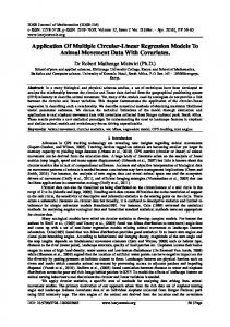
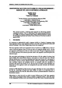
with an associated residual root mean square error of 1.12. (Our values for these coefficients differ slightly from those of Daniel and Wood because of differences in our treatment of roundoffs). Most researchers do not have the insight and perseverance of these authors. However the fitting procedure described in the previous sections applied to the original data yields similar results as we shall show. If, following the suggestion of Daniel and Wood the variable xl2 is included in the fit the residuals are further reduced. The four fits-two least-squares fits by Daniel and Wood and two robust fits are summarized in Table 5 and Table 6. Fit (1) is the original least-squares fit. The probability plot of residuals from this fit, Figure 1, suggests that 1 point (21) deserves particular

8-

from the weighted

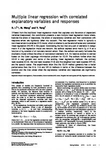
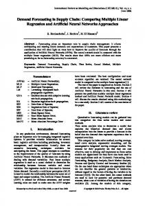
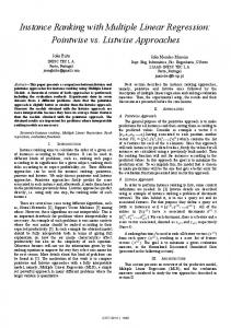
attention. Fit (2) is the least-squares fit to the data after the 4 points eventually set aside by Daniel and Wood have been removed from the fitting equation. The probability plot of the residuals, Figure 2, exhibits only slight anomalies. Fit (3) is a robust fit with c = 1.5. The probability plot of residuals from this fit, Figure 3, identifies the 4 points. Fit (4) is the same fitting procedure applied to the data with the 4 points removed. Note that the fit is unaffected by the 4 points. The probability plot of the remaining residuals, Figure 4, is comparable to Figure 2. The robust fitting procedure (3) has immediately and routinely led to the identification of 4 questionable points. The fit is independent of these points. As seen in Table 6, the coefficients of both robust fits (3 and 4) are well within the standard errors

B-

6-

.

6-

. 4-

4-

. .**

22:

.**

2 0 3 -2 @z

.**

. . -4

-

-6

-

.

l **** -4

-

-6

-

. -8

I, 1 2

I 5

I ,O

lI,IiII 20 ’ 40 ’ 60 ’ 80 30 50 70

PROBABILITY

FIGURI~ l-Probability Fit of r, , x2 , z3 TECHNOMETRICSO,

Plot

I 90

I 95

I 98 99

-8 II 1

X 100%

Residuals

from

2

I 5

I (0

IIIIII~ 20 ’ 40 ’ 60 ’ 80 30 50 60

PROBABILITY

Least-Squares

VOL. 16, NO. 4, NOVEMBER

1974

FIGURE: Z-Probability Fit 4 Points Omitted.

Plot

1’1 90 95

98 99

X ?OO%

Residuals

from

Least-Squares

A ROBUST

METHOD

FOR MULTIPLE

REGRESSION

531

the other hand the procedure is insensitive to moderate numbers of extreme observations with the result that these may be readily detected by examining residuals and further calculation with these values set aside may not be necessary. However the principal advantage lies in the detections of observations to be studied further.

. S**

6-

LINEAR

4-

10. ACKNOWLEDGEMENTS -4 -6 -I3 -

,,d 12

I IIIIII1 I I !_ 5 10 20 40 60 80 90 95 98 99 30 50 70 PROBABILITY

Downloaded by [71.74.132.239] at 00:05 11 May 2016

FIGURN 3-Probability 51 , r2 , x3

X 100%

Plot Residuals

REFERENCES from

Robust

Fit of

of the coefficients of the least squares fit (2) with points 1, 3, 4 and 21 deleted. The robust fitting procedure does not directly suggest any modifications of the original model as suggested by Daniel and Wood. However by providing residuals uncontaminated by the effects of the anomalous observations it gives the analyst a better chance to discover such improvements. 9. CONCLUSION A method for estimation and testing in robust regression has been developed. The method requires a crude, safe, initial fit which is refined to yield a procedure relatively efficient for near Gaussian data. The procedure is iterative and, compared with least-squares relatively expensive to compute. On

0-

6-

PROBABILITY

FIGIJRI~; 4-Probability 4 Points Omit ted

Plot

The author is grateful for the many helpful comments and suggestions for further investigation he has received from J. M. Chambers, C. L. Mallows and J. W. Tukey. This work was supported in part by the National Research Council of Canada. The referees have made many suggestions helpful in the revision of this paper.

X 100%

Residuals

from

Robust

Fit

PI ANDREWS,

D. F. (1971). Significance tests based on residuals. Biometrika 68, 139-148. PI ANDRICWS,D. F., BICKICL, P. J., HAMPEL, F. R., HUNICR, P. J., ROGERS, W. H. and TUKIGY, J. W. (1972). Robust Estimates of Location: Survey and Advances. Princeton Univ. Press. [31 BROWNLFX, K. A. (1965). Statistica Theory and Methodology in Science and Engineering (2nd edition) New York, Wiley. [41 DANIEL, C. and WOOD, F. S. (1971). Fitting Equations to Data, Wiley, New York. [5] DRAPER, N. R. and SMITH, H. (1966). Applied Regression Analysis, Wiley, New York. PI EFRON, B. (1969). Student’s t-test under symmetry conditions. J. Amer. Statist. Assoc. 64, 1278-1302. [71 FLICTCHICR,R. and POWELL, M. J. D. (1963). A rapidly convergent descent method for minimization. Computer J. 6, 163-168. FORSYTHE, A. B. (1972). Robust estimat,ion of straight line regression coefficients by minimizing p-th power deviations. Technometrics 14, 159-166. GAYEN, A. K. (1950). The distribution of the variance ratio in random samples of any size drawn from nonnormal universes. Biometrika 37, 236-255. [lo] GENTLEMBN, W. M. (1965). Robust estimation of multivariate location by minimizing p-th power deviation, unpublished Ph. D. thesis Princeton University. 1111GOLUR, G. H. and REINSCH, C. H. (1970). Singular value decomposition and least squares solution. Numer. Math. 14,402420. 1121HAMPEL, F. It. (1971). A qualitative definition of robustness. Ann. Math. Statist. 48,1887-1896. [I31 HU~ICR, P. J. (1964). Robust estimation of a location parameter. Ann. Math. Statist. 35, 73-101. [I41 JASCKKL, L. A. (1972). Estimating regression coefficients by minimizing the dispersion of the residuals. Ann. Math. Statist. 43,1449-1458. estimate of Il.51 JUREEKOV~, J. (1971). Nonparametric regression coefficients. Ann. Math. Statist. 42, 1328-1338. [I61MARQU,\RDT, D. W. (1963). An algorithm for leastsquares estimation of non-linear parameters. J. Sot. Ind. Appl. Math., 11, pp. 431-441. [171 RELLES, D. A. (1968). Robust Regression by Modified Least-Squares unpublished Ph.D. t,hesis Yale University. WI WILKINSON, G. N. (1970). A general recursive procedure for analysis of variance, Biometrika 57, 19-46. TECHNOMETRICSO,

VOL. 16, NO. 4, NOVEMBER

1974