the networks can be implemented on VLSI chips. First, an approximation function needs to be developed because. CMOS neural networks have an activation ...
VLSI Implementation of Neural Networks B. M. Wilamowski, J. Binfet, and M. O. Kaynak
Abstract Currently, fuzzy controllers are the most popular choice for hardware implementation of complex control surfaces because they are easy to design. Neural controllers are more complex and hard to train, but provide an outstanding control surface with much less error than that of a fuzzy controller. There are also some problems that have to be solved before the networks can be implemented on VLSI chips. First, an approximation function needs to be developed because CMOS neural networks have an activation function different than any function used in neural network software. Next, this function has to be used to train the network. Finally, the last problem for VLSI designers is the quantization effect caused by discrete values of the channel length (L) and width (W) of MOS transistor geometries. Two neural networks were designed in 1.5 µm technology. Using adequate approximation functions solved the problem of activation function. With this approach, trained networks were characterized by very small errors. Unfortunately, when the weights were quantized, errors were increased by an order of magnitude. However, even though the errors were enlarged, the results obtained from neural network hardware implementations were superior to the results obtained with fuzzy system approach.
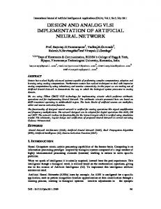
functions. Granted, other types of functions can be used, but sigmoidal type functions allow simple networks the ability to describe complex surfaces. This is due to the bell shaped derivative characteristics of a sigmoidal function. In the case presented, the neuron has a sigmoidal type activation. However, the function to describe this is not readily apparent such as the tangent hyperbolic commonly used in neural network software. This means that standard neural network training software cannot be used because it will produce incorrect solutions for the circuit realization. In the presented approach, the difficulty with VLSI neural network implementation was overcome in the following way. The “measured” activation function is used for neural network training (Section III) and the training algorithm was adapted to quantized values of weights (Section IV). II. NEURAL NETWORK CIRCUIT Nonlinear activation functions of neurons are essential for neural network operation. Such sigmoidal functions can be created in the differential pair shown in Fig. 1.
IM3 VIN
I. INTRODUCTION The analog approach is an attractive alternative for nonlinear signal processing. It provides parallel processing with a speed limited only by the delay of signals through the network. In recent years, a significant amount of research has been devoted in the development of fuzzy controllers [1]. In hardware, fuzzy systems dominate current trends in both microprocessor applications [2] and in custom designed VLSI chips [3]. Fuzzy controllers are especially useful for nonlinear systems, which are difficult to describe by mathematical models. Fuzzy controllers are also easier to implement [4][5][6][7]. Membership functions and fuzzy rules are chosen arbitrarily and therefore, fuzzy controllers are often good but not optimal. Even though neural networks are primarily implemented in software, their good approximation properties make them an attractive alternative in hardware [8][9]. One concern in hardware implementation is related to the quantized values for the weights enforced by hardware [10][11][12]. Another difficulty is caused by fact that the activation functions obtained in VLSI implementation are different from these used in neural network software. Traditionally, neurons use sigmoidal type activation
IM4 M3 M4 VX
IREF
IM2
M2
M1
Fig. 1. Sigmoidal function generated by differential pair Using a simple Shichman-Hodges MOS transistor model for strong inversion, the output currents for the MOS differential pair M3-M4 operating in strong inversion is given by:
K (VIN − V X − VTN )2 2 K 2 = (0 − V X − VTN ) 2
IM3 = IM 4
(1) (2)
and from Kirchhoff’s Law
IM 2 = IM3 + IM 4
(3)
+VDD
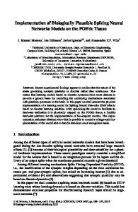
combining equations (1) through (3) one may find [13]: for
α ≤−
for
α≥
and for
1 β
1 β
−
IM 3 = 0
(4)
IM3 = IM 2
(5)
M5
Ma Ma Ma
Ma
IM3
IREF
1 1