Evaluation of TOA-Based Localization Schemes using Range Estimation at Network Layer in WLAN Environment. Shibkali Bera1 School of Mobile Computing & Communication Jadavpur University, Kolkata, India
[email protected]
Sanjoy Kumar Mondal2 Birbhum Institute of Engineering & Technology, Suri Birbhum, West Bengal, India
[email protected]
Pampa Sadhukhan3 School of Mobile Computing & Communication Jadavpur University, Kolkata, India
[email protected]
Abstract- A lot of wireless localization schemes using time of
is that it would incur a lot of expenses and face some
arrival (TOA) have been proposed in the literature with
technical challenges to replace the existing handset with
comprehensive performance comparisons in terms of accuracy, complexity and robustness. The major issue in TOA-based localization schemes is that the presence of error due to nonline-of-site (NLOS) propagation in the range measurements
GPS-equipped handsets. Thus, a lot of researchers have concentrated on network based localization [2] that does not require any changes to the existing handsets and utilizes the
introduces a lot of errors in location estimation. Thus we have
existing network infrastructure, i.e. cellular system or WLAN
focused on those TOA-based localization schemes that can
system to estimate the position of the Mobile Station (MS).
mitigate the effect of NLOS errors to provide reasonable location
accuracy.
Another
major
issue
in
TOA-based
localization is the computational complexity incurred by solving
Network-based localization using time-of-arrival (TOA), time difference-of-arrival (TDOA), angle-of arrival
the non-linear equations associated with the location estimation.
(AOA) and received signal strength (RSS) have been
Thus, among the various TOA-based localization schemes that
extensively reviewed in [2], [3], [4]. In RSS based technique,
work in NLOS environment, we have chosen two-step least
the distance between the MS and base station (BS) or access
square (LS) method for estimation of location of a mobile user
point (AP) is measured by the attenuation of signal
in WLAN environment. To the best of our knowledge, no such
propagated between the MS and the BS or AP. The accurate
real evaluation of two-step LS method does exist in literature. In this paper, we have proposed a novel technique for estimation of round trip time (RTT) between the Base Station (BS) and the Mobile Station (MS) of Internet Control Message Protocol (ICMP) packet in order to avoid the requirement for exact
distance measurement depends on the radio propagation model that defines how signal strength reduces with distance traversed by the signal. The continuously varying signal propagation condition makes the RSS-Based localization
synchronization between the MS and the BS. Our proposed
technique obsolete in outdoor environment. On the other
technique also shows a statistical post-processing step to reduce
hand, pattern matching localization technique based on RSS
the errors incorporated into TOA measurements. Moreover, in
requires constructing and maintaining a fingerprint database
this paper we have compared the performance of two-step LS
for a particular area that is very time consuming and
method in theoretical environment with that in WLAN
laborious. Among other localization techniques, Time
environment.
Difference
of
Arrival
(TDOA)
requires
precise
Keywords: Time-of-Arrival (TOA), Base Station (BS), Mobile
synchronization between the BSs whereas a small error in
Station (MS), Two-Step Least Square (Two Step LS), Wireless
angle measurement would produce a large amount of location
Local Area Network (WLAN). Average Location Errors (ALE)
estimation error in case of Angle of Arrival (AOA). Thus, we mainly focus on TOA-based localization techniques in this
I. Introduction
paper because the measurement of signal propagation time
Wireless localization has gained a lot of popularity as it is
between the BS and the MS from round trip time (RTT)
essential for providing location-based services such as
measurement does not require the precise synchronization
location sensitive billing, location-based routing, and
between the BS and the MS. However, the major issues in
intelligent transportation system and so on. Although, it is
TOA-based localization techniques are that the range
possible to estimate the location of a mobile user accurately
measurements contain errors due to system measurement
using Global Positioning System (GPS), it does not work
noises and non-line-of-sight (NLOS) propagation caused by
well in indoor areas because of its very poor signal strength.
blockage of direct path between the BS and MS. The large
Another problem with the wide use of GPS-based positioning
positive bias of NLOS error makes the range measurement
1
978-1-4577-1328-6/11/$26.00 2011 IEEE
larger than the true distance between the MS and the BS. A lot of TOA-based localization schemes that can mitigate the effect of NLOS propagation have been proposed in [5-9], [11] and [12]. However a major issue in these TOA-based localization schemes working under NLOS environment is the computational complexity incurred by solving the nonlinear equation associated with the location estimation of MS. Thus to avoid the heavy computation required to solve the
II. Overview of Two-step LS method: In this section, we have explored the two-step LS method proposed in [10] in brief. The two-step LS method estimates two-dimensional (2D) location of the MS from a set of TOA measurements under the presence of NLOS errors and a small amount of system measurement errors. The algorithm is divided into two steps and it has been described below.
non linear equations, we have chosen the localization method
y
proposed in [10] that only needs two computing iterations to
MS (x , y)
estimate the position of the MS under presence of NLOS error. To demonstrate the validity of above-mentioned localization method known as two-step least square (LS), authors in [10] have provided simulation results only by considering the error due to system measurement noise as a
BS (xi , yi )
Gaussian random variable with zero mean and the amount of NLOS errors incorporated into the set of measured distance
x
Fig.1 Localization in 2-D plane
as a constant positive value. In these simulations, measured distances between the MS and the BSs are generated by
Considering, (x, y) is the position of the MS and (xi, yi) is the
adding systems measurements errors and NLOS errors to the
position of the ith BS as shown in Fig. 1 and di is the
true distance between the MS and the BS. Thus, this sort of
measured distance between ith BS and the MS, which is
simulations does not guarantee that the algorithm would
always larger than the true distance between ith BS and the
achieve desired location accuracy in real environment. To the
MS in presence of NLOS errors, we obtain the following set
best of our knowledge, no evaluation of the above mentioned
of equations
localization scheme have been made in real environment, i.e.,
di2 ≥ (xi – x)2 + (yi – y)2
cellular network or WLAN environment. Thus in this paper,
= Ki – 2xix – 2yiy + x2 + y2 for i= 1,2,3 ,.., M……………..(1)
our aim is to evaluate the performance of the localization scheme proposed in [10] in WLAN environment by
Where, M is the number of BSs and Ki = xi2+yi 2
estimating the TOA measurement from the RTT of signal
After replacing x2+y2 by R, the following set of linear
propagated between the MS and the BS that is part of WLAN
equations are obtained
infrastructure
to
avoid
the
necessity
of
precise
synchronization between the BS and the MS. This paper is organized as follows. Section II presents an overview of two-step LS method and performance evolution
– 2xix – 2yiy + R≤ di2 - Ki for i = 1, 2, 3,….., M…………..(2) Considering Za =[x, y, R]T , equation (2) can be rewritten as Ga*Za ≤ h ,…………………………………………..…….(3)
of the method in simulation environment. The proposed technique for estimation of time delay or TOA in WLAN
Where,
2
environment is presented in section III. Section IV provides requirements and experimental testbed for Two-Step LS
h=
method is discussed and after that Experimental results and comparison between evaluated results and simulated results for above method are analyzed. Finally section V presents the conclusion and our future scope of research.
d1 - K1 2 d2 - K2 : : : : 2 dM - KM
Ga =
-2x1 -2x2 -2xM
-2y1 1 -2y2 1 : : -2yM 1
In case of LOS propagation between the MS and the BSs and if there is no system measurement error the equation (3) turns into equalities.
The intermediate location estimation of the MS after the first step of two-step LS method can be obtained as follows Za = (GaT Ψ-1 Ga)-1 GaT Ψ-1 h ……………….. (4)
among the above factors. According to the graphical representation it is shown that, when the number of BSs is changed from 5 to 10, then the value of ALE is changed 150 meter to 100 meter. So, from this graphical result it is cleared
Where, Ψ=4c2 BQB and B=diag {d1, d2,…..dM} and c is
that to improve the accuracy, it should necessary to increase
speed of signal propagation
the number of BSs.
Here Q is the Covariance matrix of measured noise. After obtaining the initial location estimation of the MS, the final location estimation of the MS can be obtained as follows Zf =[x2 y2]T =(Ga’ T Ψ ‘- 1 Ga ‘)-1 Ga’ T Ψ ‘- 1 h’ …………….(5) Where
[Za]12 h’ = [Za]22 [Za]3
G a’ =
1 0 0 1 1 1
Zf =[x2
y2]T
Now, Ψ’ = 4c2 B’QB’......................................................(6) Where B’ = diag {x0, y0, 0.5}
Fig.3. Average Location Errors (ALEs) are changed with Noise (N) in case of theoretical evaluation Two Step Least Square method.
Fig. 3 shows that ALEs increase slightly, when the So the final location estimate of the MS is Zp = √ Zf
…………………………...…….………(7)
Performance evolution in simulation environment: In the simulation, the average location error (ALE) is calculated by using following equation. 0 2
0 2
ALE = [√ {(x – x ) + (y – y ) }]….................(8) Where, (x, y) is the estimated position of MS and (x0, y0) is the original position of the MS.
power of noise increases, and it increase largely as the NLOS interference increases. III. Proposed Technique for Estimation of TOA in WLAN Environment: This section presents our proposed technique for estimation of time delay or TOA from the round trip time (RTT) taken by network-layer packet in order to avoid the need for precise synchronization between the MS and BS. Mobile station TTX data packet
Base Station Tp datapacket
tPROC data packet Fig. 2 Average Location Errors changed with the number of BSs (M) in
RTT
tP ACK
theoretical evaluation of two step LS method. Fig.4 RTT measurement using IEEE 802.11 data/ACK
The variance in system measurement noise denoted 2
2
packets RTT is the time taken by a signal to travel from transmitter to
as (σ ) is considered 100 m and the maximum number of
a receiver and return back. We have estimated RTT in
BSs is assumed ten and the possible maximum error (N) is
between MS and BS by measuring the time elapsed between
considered as 300 m. In Fig. 2 it is shown that the ALEs
sending a packet (Ttx data packet) from the network layer and
decrease slightly as the number of BSs increases. This means
reception of the corresponding acknowledgement packet
that the number of BSs plays a dominating role in the ALEs
(Tp ACK) as seen in Fig.4.
So, the measured Toa(τi) at ith BS is
τi =
TRTT
BS. Then from ten RTT values, average RTT is computed. By using the average RTT the distance between MS and ith
………..……………….(9)
2
BS is estimated.
Where, TRTT is the total RTT measurement. But this τi consist
Y
various delays i.e., processing delay, routing delay, queuing delay etc. For that reason the value of τ is increased, so that
.
BS6
the error in distance measurement will be highly increased. If
( 0,8)
BS7 ( 4, 8 )
BS8 (8,8)
these errors are reduced from the measure RTT then the effective
propagation
time
(τe)
is
calculated
from
BS4 (0, 4)
equation (11)
τe =
TRTT – 2 TPROC – 2 TQUE 2
………………(10)
BS5 (8,4)
X’ BS1 ( 0, 0)
BS9
Where, TPROC is the processing time and T QUE is the queuing
MS ( 4 , 4) )
( -4, 0
)
BS2 ( 4,0 )
X BS3 (8,0)
BS10 ( 0 , -4)
time. So, we can get the measured distance (di) between BS
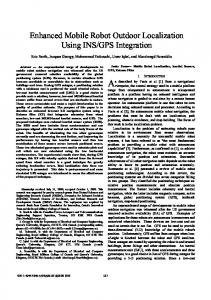
Y’ Fig. 5 The position of BSs and MS during experiment to measure
and MS.
RTT in Two-Step LS method
di = τi * c ……………………………………….(11) Where, c is the propagation speed of signal and τi is the
IV.b Experimental results and comparison between evaluated results and simulated results for Two-Step LS method:
After measuring RTTs in a sequence between the
corresponding TOA measurement at ith BS.
MS and each BS, average RTT is computed and it is shown IV: Performance evaluation of two-step LS method in WLAN environment:
in Table 1. From the average RTT values measured distance between the BSs and MS is computed using equation 10.
The experimental testbed is required to evaluate two-step LS
Table 1 shows the values for average RTT and measured
method consist ten BSs and one MS and it is shown in
distance between each BS and MS that is located at fixed
Fig.
5. The position of each BS and the system configuration of the BSs and the MS provided in section IV.a and section IV.b provide the experimental result and then compares between evaluated results and simulated results for two-step LS method. IV.a Requirements and Experimental Testbed for Two-Step LS method:
position (4, 4). BS’s position (xi,yi)
MS
Avg RTT
Measured
position
(in ms)
distance
1.(0,0)
0.002989956
448m
2. (4,0)
0.002853606
428m
3. (8,0)
0.003010806
462m
0.002808156
421m
(4, 4)
The following devices have been used as BSs and
4.(0,4)
MS:- notebook, HP Compaq 2230s, Intel(R) Core™ 2 duo
5. (8,4)
0.002880006
432m
6.(0,8)
0.003035406
455m
7.(4,8)
0.002899056
434m
8.(8,8)
0.002898956
414m
Table 1. Now
9.(-4,0)
0.003391332
508m
they are all connected in an adhoc network. The MS is
10.(0,-4)
0.003401223
510m
CPU T5870,2.00 GHz, 956 MB of RAM running in Fedora 10. To evaluate the Two-Step LS method in WLAN environment, ten BSs and one MS are considered as shown in Fig. 5. The positions of ten BSs are given in
randomly positioned along the line y=4. A software routine is developed into all BSs and MS to measure RTT between BS and MS where the MS takes ten RTT measurements to every
Table 1: Distance measurement from RTT in WLAN environment
The measured distances between each BS and the MS shown
In
WLAN
environment
(SMCC
LAB,
Jadavpur
in Table1 incorporate additional error due to queuing delay and
University), to improve the location estimation accuracy in
processing delay at the network layer and data link layer.
WLAN environment, there are considered same scenarios as
Thus, to remove these additional errors, we have taken the help of another system that is called reference BS (Ref. BS). The Ref. BS is placed very near to the MS to measure average RTT between the Ref. BS and the other BSs as shown in
Table 2.
The Ref_RTT basically indicates the additional queuing & processing delay incorporated into RTT measured between the BSs and the MS. Ref_RTT can be represented by the following equation. Ref_RTT = 2*(TProc + TQue)…………………….…………..(12)
well as real evaluation of two-step LS method. Additionally one BS is considered as a Reference BS (BSr) which is placed as close as possible to MS’s position. Now they are all connected in adhoc networking mode where the MS takes ten RTT measurements to every BSs and the Reference BS. Then from ten RTT values, average RTT and reference RTT are calculated. After that the reference RTT is subtracted from the average RTT of ith BS. By using the subtracted RTT the distance between MS and ith BS are calculated. The measured distance between BS and MS from using this algorithm consists less noise.
Thus, effective propagation time (τe) can be obtained as follows τe =(TRTT – Ref_RTT) /2 …………………..………………(13) Table 2 shows the measured distance between each BS and MS computed using equation 13. Fig. 6 shows how the ALE varies in Two-Step LS method
A data set is given below to calculate the measured distance by using equation (10) and (11).
BSs PosiTion
MS
Avg_RTT (in ms)
1.(0,0)
0.002989956
2.(4,0)
0.001753334
Ref _RT T
Trans_ RTT (in ms) .0004054
Measured distan -ce 60m
.00026905
40m
.00049625
74m
.0002236
33m
.00029545
44m
while the number of BSs (M) is changed in simulation and real evaluation.
3.(8,0)
(4,4)
0.003080988
0. 00 25 84 55 64
4.(0,4)
0.002107793
5.(8,4)
0.001979787
6.(0,8)
0.002709315
.00045085
67m
7.(4,8)
0.001898871
.0003145
39m
8.(8,8)
0.002998775
.0003144
47m
9.(-4,0)
0.003391332
.0008067
121m
10.(0,-4)
0.003401223
.0008166
122m
Fig. 6 Comparison both results in case of ALEs, when the number of BSs (M) is changed.
It is evident from Fig. 6 that when the number of BSs is
Table 2: distance measurement from RTT in WLAN environment using reference Base Station
increased then the ALE will be gradually decreased. That means due to increase the number of BSs the location finding
Comparative study between the two methods in WLAN
accuracy will be higher because the value of ALEs are
environment.
decreased. But it is shown from the above figure, in real
By doing the real evaluation of the two methods it
environment the rate of decreasing ALEs is less than the
is shown that the ALE is proportional to increase with the
simulated scenario as per BSs number increased due to some
noise variance i.e. when noise variance is high the value of
additional error in real environment which are not considered in
ALE is also high as shown as Fig. 7. But with compare to
simulation environment.
both methods it is cleared that in a certain noise variance the value of ALE of two-step LS Method without using Ref. BS
is higher than the value of ALE in two-step LS method using
Finally it is concluded that the measured distance using
Ref.BS.
reference BS is less noisy than the measured distance without
It proves that using Ref. BS provides more accuracy to find
using Reference BS.
the MS position because in this method there is no concept of reference BS.
tprop =
(Total_RTT – RTT_Reference BS) 2
Section V: Conclusion and Future Scope During measurement of RTT in Network level, sending first packet may take more time and in some networks, the first packet will often be lost. This problem could be avoided by sending more than one packet and it should better to ignore the results for the first packet. In this paper evaluated algorithms for indoor localization technique only consider the static object not the mobility of the object in dynamic environment. In future it can be extended for localization of a Fig. 7 Comparison of ALEs changed with Noise Variance (N) between using Ref BS vs without using Ref BS.
During experiment MS sends the ICMP packet to different BSs to calculate the RTT. Actually, Total_RTT = {Processing time + Propagation time + queuing time + processing time + transmission time (ack) + queuing time} Where, processing time means the time difference between packet ready for sending and just before packet sending time. Queuing time means, when the transmitted packet is store in receiver queue but receiver did not receive it or read it, this waiting time in queue is known as queuing time. It may be considered that the processing time and queuing time are equal of all BSs like reference BS. So, it should necessary to keep the BSr as close as possible to MS., for which the propagation time is considered tens to zero ms. That means the Total_RTT of reference Base Station consists of only processing time, queuing time and very less propagation time and other various type of delays. When, the RTT is measured in WLAN environment according to Two-Step LS method, there is no reference Base Station. So it is not possible to subtract the processing time and queuing time from Total_RTT. So, the error in measured distance is obviously high in case of without using reference BS whereas using reference BS method, the processing time and queuing time is subtracted from Total_RTT, so that the effective propagation (tprop) time can easily be obtained. Now, by using the tprop and signal propagation speed (c) the distance between MS and BS are calculated.
mobile device in dynamic environment. References: [1]. Revision of the Commissions Rules to Insure Compatibility with Enhanced 911 Emergency Calling Systems. Federal Communications Commission (1996) [2] A. H. Sayed, A. Tarighat, and N. Khajehnouri, “Network-based wireless location,” IEEE Signal Processing Mag., vol. 22, no. 4, pp. 24–40, July,2005. [3]. Rantalainen, T.: Mobile Station Emergency Location in GSM. In: Proc. IEEE International Conference Personal Wireless Communication (PWC 1996), New Delhi, India, February 1996, pp. 232–238 (1996) [4]. Chan, Y., Ho, K.: A simple and efficient estimator for hyperbolic location. IEEE Trans. Signal Processing 42(8), 1905–1915 (1994) [5] P. C. Chen, “A non-line-of-sight error mitigation algorithm in location estimation,” in Proc. IEEE Int. Conf. Wireless Communication. Networking (WCNC), vol. 1, New Orleans, LA, Sept. 1999, pp. 316–320. [6] S. Gezici and Z. Sahinoglu, “UWB geolocation techniques for IEEE 802.15.4a personal area networks,” MERL Technical report, Cambridge, MA, Aug. 2004. [7] Y.T. Chan, W. Y. Tsui, H. C. So, and P. C. Ching, “Time of arrival based localization under NLOS conditions,” IEEE Trans. Veh. Technol., vol. 55, no. 1, pp. 17–24, Jan. 2006. [8] W. Kim, J. G. Lee, and G. I. Jee, “The interior-point method for an optimal treatment of bias in trilateration location,” IEEE Trans. Veh. Technol., vol. 55, no. 4, pp. 1291–1301, July 2006. [9] Z. Li, W. Trappe, Y. Zhang, and B. Nath, “Robust statistical methods for securing wireless localization in sensor networks,” in Proc. IEEE Int. Symp. Information Processing in Sensor Networks (IPSN), Los Angeles, CA, Apr. 2005, pp. 91–98. [10] X. Wang, Z. Wang, and B. O. Dea, “A TOA based location algorithm reducing the errors due to non-line-of-sight (NLOS) propagation,” IEEE Trans. Veh. Technol., vol. 52, no. 1, pp. 112–116, Jan. 2003. [11]. Venkatraman, S., Caffery Jr., J., You, H.R.: A Novel ToA Location Algorithm Using LoS Range Estimation for NLoS Environments. IEEE Trans. Vehicular Technology 53(5), 1515–1524 (2004) [12]. Liao, J.F., Chen, B.S.: Robust Mobile Location Estimator with NLOS Mitigation Using Interacting Multiple Model Algorithm. IEEE Trans. Wireless Comm. 5(11), 3002–3006 (2006) [13] F.Barcelo-Arroyo, M.Ciurana , I. Watt, F. Evanou, L. De Nardis, P. Tome,”Indoor location for safety applications using wireless networks,” University politecnica de Catalunya,France Telecom and R&D, University of Rome La Sapienza , Swiss Federal Institute of Technology.