Blucher Mechanical Engineering Proceedings May 2014, vol. 1 , num. 1 www.proceedings.blucher.com.br/evento/10wccm
A Feed Forward Neural Network in CUDA for a Financial Application Roberto Bonvallet1 , Cristi´an Maureira1 , C´esar Fern´andez1 , Paola Arce1 , Alejandro ˜ 2. Canete 1
Informatics Department, Universidad T´ecnica Federico Santa Mar´ıa. Corresponding address: (
[email protected]). 2 IFITEC, Financial Technology. Abstract. Feed forward neural networks (FFNs) are powerful data-modelling tools which have been used in many fields of science. Specifically in financial applications, due to the number of factors affecting the market, models with a large quantity of input features, hidden and output neurons can be obtained. In financial problems, the response time is crucial and it is necessary to have faster applications which respond quickly. Most of the current applications have been implemented as non-parallel software running on serial processors. In this paper, we show how GPU computing allows for faster applications to be implemented, taking advantage of the inherent parallelism of the FFN in order to improve performance and reduce response time. The problem can be conveniently represented by matrix operations implemented using the CUBLAS library. It provides highly optimized linear algebra routines that take advantage of the hardware features of the GPU. The algorithm was developed in C++ and CUDA and all the input features were received using the ZeroMQ library, which was also used to publish the output features. ZeroMQ is an abstraction over system sockets that allows chunks of data to be efficiently sent minimizing the overhead and system calls. The algorithm was tested on an NVIDIA M2050 graphics card with a Intel Xeon X5650 2.67GHz CPU for a neural network of 1000 input features, 2000 hidden neurons and 500 output neurons. Response times of the order of 900 µs were obtained. Keywords: high-frequency trading, GPU programming, neural networks. INTRODUCTION The quick development of computational power has allowed markets to speed up the number of transactions executed every day in the electronic markets, generating a huge amount of intraday financial data. As a consequence, the study of HighFrequency Trading (HFT) algorithms [2, 5, 6] has risen to become one of the main tools for quantitative analysts. HFT is the use of technological tools to trade all kind of securities in a short period of time, from seconds to milliseconds. Nowadays, trader strategies are based on complex quantitative models which provide useful information to make a decision about when to enter or exit the market.
Because of the large amount of information and complex algorithms to be executed, High-Performance Computing (HPC) provides tools (hardware and software) that are indispensable to accelerate computation. In particular, GPU computing [9] has become the industry standard for fast options pricing, risk analysis and algorithmic trading. GPUs provide massive parallelism and high memory bandwidth at a affordable cost, practically turning a standard compute server into a supercomputer. Furthermore, the architecture of the GPU maps well to the kind of computations that are usually needed by HFT algorithms. One of the most used learning algorithms in HFT are Feed Forward Neural Networks (FFNs), which are a widely-used frameworks for learning tasks such as regression, classification and clustering problems [7, 3]. Due to the volatile behavior of the financial time series, the models generated using neural networks are usually large and require lots of calculation. The use of large amounts of data, calculations and response time needed are more than sufficient reasons to use GPU computing to achieve responses in a short period of time. Moreover, the use of the ZeroMQ library allows the sending and receiving of data efficiently. In the next sections we will present a literature review, details of the FFN representation and the architecture of the solution. Also, technical details of the application, experimental results and our final conclusions are given. LITERATURE REVIEW Neural networks algorithms have been extensively used in many fields of science: forecasting, image processing, pattern recognition, etc. When the models generated have a large number of neurons and connections, the number of calculations increase and also the time needed to obtain an answer. In order to achieve better response time of the network output, some approaches has been proposed taking advantage of how easy it is to parallelize them [1, 4] and specifically some of them have been applied to financial applications [12, 11, 8]. Recently, some of neural networks parallel algorithms have been implemented using GPU [10].
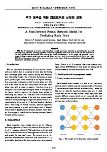
MODEL FORMULATION Feed Forward Network Architecture Feed Forward neural networks (FFN) have three layers: input, hidden and output layer. A graphical representation of the FFN can be seen in figure 1:
Figure 1. Feed Forward Network diagram. Each layer of the FFN has a set of neurons and the connections between them will be conveniently represented as matrices: W: This matrix stores all the weights between the input and the hidden neurons, i.e. wi,j is the weight between the hidden neuron i and the input neuron j:
Wh×n+1
w1,1 · · · .. ... = . wh,1 · · ·
w1,n w1,n+1 .. .. , . . wh,n wh,n+1
where h is the total number of hidden neurons, n is the number of inputs (number of features) and the last column has the biases of the hidden neurons. ∆: This matrix stores the weights between the input and the hidden layer, i.e. δi,j is the weight between the output neuron i and the hidden neuron j:
∆ m × h +1
δ1,1 · · · .. ... = . δm,1 · · ·
δ1,h .. . δm,h
δ1,h+1 .. , . δm,h+1
where m is the number of outputs, h the total number of hidden neurons and the last column has the biases of the output neurons. Therefore, the input ηi of every hidden neuron i can be obtained as: ! ηi = Φ
n
∑ wi,j x j + biasi,1
j =1
,
where wi,j is the weight of the link between the hidden neuron i and the input x j . The function Φ is the activation function. In this work the hidden and output layer have the logistic sigmoid function defined as: Φ( x ) =
1 1 + e− x
The input γi of every output neuron i is: γi = Φ
h
∑ δi,j ηi + biasi,2
! ,
j =1
where δi,j is the weight of the link between the output neuron i and the hidden neuron output j. Procedure The output of the FFN is obtained through matricial representation of the problem. The input of the problem is a vector with n features: x1 .. X= . xn 1 In order to simplify the implementation, a feature with value 1 is added at the end of the vector in order to account for the biases that are stored in the last column of each weight matrix. The following steps explain in detail our implementation: Step 1: the input of the hidden layer inputs is computed as the linear combination between weights and inputs, i.e: n +1
ηi =
∑ wi,j x j
j =1
In matricial form: η1 w1,1 · · · .. .. .. H = . = Wh×n+1 = . . wh,1 · · · ηh
w1,n w1,n+1 .. .. . . wh,n wh,n+1
x1 . .. × xn 1
Step 2: the activation function of hidden neurons is applied to every component of H: Φ ( η1 ) H = ... Φ ( ηh )
Step 3: in order to account for the bias in the output layer a new component with value 1 is added to vector H: η1 .. H=. ηh 1 Step 3: the input of output neurons is computed as the linear combination between weights and vector H from step 2. Let us define: h
γi =
∑ δi,j ηj
j =1
in matricial form:
γ1 δ1,1 · · · .. .. .. Γ= . = . . δm,1 · · · γm
δ1,h .. .
δ1,h+1 .. .
δm,h δm,h+1
η1 .. . × ηh 1
Step 4: the activation function of output neurons is applied to every component of Γ: Φ(γ1 ) Γ = ... Φ ( γm ) The vector Γ is the output we are looking for. Pseudocode The algorithm 1 shows the representation of the problem using matrices. This algorithm is executed for each arriving input vector. Algorithm 1 Get Output of FFN Require: X, W, ∆ Ensure: Γ H←W×X H ← Φ(H) Γ←∆×H Γ ← Φ(Γ)
IMPLEMENTATION DETAILS CUBLAS CUBLAS is the CUDA library which implements BLAS (Basic Linear Algebra Subprograms), and provides several optimized algebra routines. In the present study, the Matrix-Vector multiplication operation is used (cublasSgemv).
Considering that the two stages of the algorithm generates the hidden and the output vector consists in a Matrix-Vector multiplication, it is necessary to use the GPU in the most efficient way, and CUBLAS provides such a scenario. ZeroMQ The current message-passing implementation based on the ZeroMQ library has the following details. Transport: TCP transport is used because it is one of the best transport methods implemented in the last version of ZeroMQ. Infrastructure: The Queue infrastructure is used to implement a client/server model. Messaging pattern: The Request/Response model was selected, which is a unidirectional communication from a client to servers. This model implies synchronization between the send() and the recv() method, ensuring that no messages will be lost.
Figure 2. ZeroMQ interaction diagram. The current version uses some default values to make the connection between the clients and servers. EXPERIMENTAL RESULTS All the experiments were performed on a computer with the following technical details: • Intel Xeon CPU E5520 @ 2.27GHz • 12 GB RAM • nVidia Tesla C1060.
• OS: Scientific Linux SL release 5.6 (Boron) We present the results of a set of experiments which aims to describe the performance associated with different sizes of the Input Layer (N), the Hidden Layer (H) and the Output Layer (O) of the neural network. Each configuration was executed 1000 times, and the table information consist in: ¯ • Average time (x) • Standard deviation (σ) • Best time (xbest ) • Worst time (xworst ) There are two important times measured in this experiments, the Message time and the GPU time, which are represented in the interaction diagram (figure 2). The Execution time represent the Message time, and the GPU calculation represent the GPU time.
Configuration ID N H O 1 1000 1000 1000 2 1000 1000 2000 3 1000 1000 3000 4 1000 2000 1000 5 1000 2000 2000 6 1000 2000 3000 7 1000 3000 1000 8 1000 3000 2000 9 1000 3000 3000 10 2000 1000 1000 11 2000 1000 2000 12 2000 1000 3000 13 2000 2000 1000 14 2000 2000 2000 15 2000 2000 3000 16 2000 3000 1000 17 2000 3000 2000 18 2000 3000 3000 19 3000 1000 1000 20 3000 1000 2000 21 3000 1000 3000 22 3000 2000 1000 23 3000 2000 2000 24 3000 2000 3000 25 3000 3000 1000 26 3000 3000 2000 27 3000 3000 3000
Message measures [sec] x¯ σ xbest xworst 0.00026 7.706e-05 0.00020 0.00126 0.00022 8.335e-05 0.00017 0.00090 0.00020 3.545e-05 0.00020 0.00070 0.00023 9.410e-05 0.00018 0.00107 0.00021 5.426e-05 0.00016 0.00101 0.00024 7.083e-05 0.00018 0.00105 0.00025 7.974e-05 0.00020 0.00148 0.00025 5.646e-05 0.00020 0.00091 0.00022 5.065e-05 0.00018 0.00071 0.00017 2.287e-05 0.00016 0.00047 0.00072 4.565e-05 0.00067 0.00158 0.00086 5.293e-05 0.00081 0.00167 0.00113 9.086e-05 0.00097 0.00216 0.00118 5.286e-05 0.00109 0.00202 0.00153 8.577e-05 0.00141 0.00220 0.00145 8.497e-05 0.00130 0.00219 0.00180 8.466e-05 0.00167 0.00257 0.00215 7.700e-05 0.00206 0.00344 0.00088 6.053e-05 0.00077 0.00171 0.00103 9.117e-05 0.00091 0.00233 0.00127 0.0001020 0.00110 0.00252 0.00134 8.465e-05 0.00124 0.00224 0.00178 9.634e-05 0.00162 0.00233 0.00189 9.211e-05 0.00172 0.00252 0.00195 8.170e-05 0.00185 0.00257 0.00228 6.506e-05 0.00210 0.00300 0.00258 5.440e-05 0.00245 0.00327
Table 1. Message measure information
ID 1 2 3 4 5 6 7 8 9 10 11 12 13 14 15 16 17 18 19 20 21 22 23 24 25 26 27
Configuration N H O 1000 1000 1000 1000 1000 2000 1000 1000 3000 1000 2000 1000 1000 2000 2000 1000 2000 3000 1000 3000 1000 1000 3000 2000 1000 3000 3000 2000 1000 1000 2000 1000 2000 2000 1000 3000 2000 2000 1000 2000 2000 2000 2000 2000 3000 2000 3000 1000 2000 3000 2000 2000 3000 3000 3000 1000 1000 3000 1000 2000 3000 1000 3000 3000 2000 1000 3000 2000 2000 3000 2000 3000 3000 3000 1000 3000 3000 2000 3000 3000 3000
x¯ 3.786e-05 3.525e-05 3.303e-05 3.797e-05 3.324e-05 3.473e-05 3.179e-05 3.571e-05 3.927e-05 3.013e-05 0.00051 0.00061 0.00072 0.00089 0.00111 0.00106 0.00140 0.00173 0.00059 0.00070 0.00078 0.00101 0.00121 0.00142 0.00151 0.00184 0.00218
GPU measures [sec] σ xbest 1.216e-05 3.219e-05 8.488e-06 2.672e-05 2.607e-06 2.733e-05 1.201e-05 2.943e-05 3.784e-06 2.871e-05 6.405e-06 3.064e-05 3.728e-06 2.874e-05 5.986e-06 3.172e-05 8.036e-06 2.691e-05 4.261e-06 2.693e-05 8.916e-06 0.00049 7.287e-06 0.00059 1.768e-05 0.00069 1.069e-05 0.00087 1.782e-05 0.00108 1.872e-05 0.00103 1.999e-05 0.00135 2.181e-05 0.00169 6.893e-06 0.00057 1.921e-05 0.00065 1.540e-05 0.00076 1.222e-05 0.00098 2.250e-05 0.00116 2.285e-05 0.00137 1.862e-05 0.00148 2.624e-05 0.00178 2.682e-05 0.00213
Table 2. GPU calculation measures information
xworst 0.00027 9.226e-05 9.436e-05 0.00026 9.327e-05 9.392e-05 9.912e-05 9.323e-05 0.00010 7.310e-05 0.00063 0.00068 0.00083 0.00097 0.00121 0.00129 0.00149 0.00183 0.00066 0.00092 0.00090 0.00113 0.00134 0.00156 0.00161 0.00200 0.00231
(a) Message time average
(b) Message time standard deviation
(c) Message time best
(d) Message time worst
Figure 3. Message time figures
(a) GPU time average
(b) GPU time standard deviation
(c) GPU time best
(d) GPU time worst
Figure 4. GPU time figures Considering the Average plots 3a 4a, we can predict the results due the amount of operation in the current implementation: The Input vector has N values, the Input-Hidden matrix has NxH elements, the Hidden vector has H values, the Hidden-Output matrix has HxO elements, and finally
the Output vector has O values, so the total amount of operation is H · ( N 2 + H · O). A more explicit idea of the operations amount of each configuration is described in the following plot.
Figure 5. Amount of operation of each configuration experiment The only difference is the first nine experiments, which consist in a certain amount of operations but distributed in a similar way, which give us a similar execution time. Considering the Standard deviation, we can observe in the case of the message time 3b, almost all the experiments has a similar behavior, but taking into account the last set of experiments, increasing the operation numbers, the time is close to the mean. In the other hand, the GPU time 4b, which consist in the GPU calculation process, increasing the operation numbers, the obtained values are increasingly distant from the mean. CONCLUSION The present work presents a simple but efficient approach to parallel neural processing by means of GPU computing. The forward pass processing was mapped to matrix-vector multiplications in order to increase the performance and response time based on the CUDA implementation of the BLAS interface. In virtue of the nature of matrix-vector multiplication algorithm (fine-grained), the GPU computing is suitable to perform the computations on large size problems. Thanks to ZeroMQ library, the network message passing does not become a critical factor given his performance, therefore, it delivers us an efficient communication library for high frequency data. Despite of low communication network performance (Ethernet) and to use the same machine for the sending and receiving financial informacion, the approach takes advantages in large scenarios, for instance, when N, H and O have the same value, of 3000, the difference between the message time and the gpu time is about 0.00040[sec], an interesting result taking on account the problem sizes. The previous facts reveal that an approach based on GPU and ZeroMQ could become in a framework for neural processing on high frequency data.
1. REFERENCES References [1] S.W. Aiken, M.W. Koch, and M.W. Roberts. A parallel neural network simulator. In Neural Networks, 1990., 1990 IJCNN International Joint Conference on, pages 611 –616 vol.2, jun 1990. [2] Irene Aldridge. High-Frequency Trading: A Practical Guide to Algorithmic Strategies and Trading Systems (Wiley Trading). Wiley, 2009. [3] Christopher M. Bishop. Neural Networks for Pattern Recognition. Oxford University Press, USA, 1996. [4] Alexandra I. Cristea and Toshio Okamoto. A parallelization method for neural networks with weak connection design. In Proceedings of the International Symposium on High Performance Computing, ISHPC ’97, pages 397–404, London, UK, UK, 1997. Springer-Verlag. [5] M. M. Dacorogna, R. Gencay, U. Muller, R. B. Olsen, and O. V. Olsen. An introduction to high frequency finance. Academic Press, New York, 2001. [6] Michael Durbin. All About High-Frequency Trading (All About Series). McGrawHill, 2010. [7] Kevin Gurney. An Introduction to Neural Networks. CRC Press, 1997. [8] Wei Huang, Kin Keung Lai, Yoshiteru Nakamori, Shouyang Wang, and Lean Yu. Neural networks in finance and economics forecasting. International Journal of Information Technology & Decision Making (IJITDM), 06(01):113–140, 2007. [9] David B. Kirk and Wen mei W. Hwu. Programming Massively Parallel Processors: A Hands-on Approach (Applications of GPU Computing Series). Morgan Kaufmann, 2010. [10] KS Oh and K Jung. GPU implementation of neural networks. PATTERN RECOGNITION, 37(6):1311–1314, JUN 2004. [11] Rashedur M. Rahman, Ruppa K. Thulasiram, and Parimala Thulasiraman. Performance analysis of sequential and parallel neural network algorithm for stock price forecasting. International Journal of Grid and High Performance Computing (IJGHPC), 3(1):45–68, 2011. [12] Ruppa K. Thulasiram, Rashedur M. Rahman, and Parimala Thulasiraman. Neural network training algorithms on parallel architectures for finance applications. Parallel Processing Workshops, International Conference on, 0:236, 2003.