HAIT Journal of Science and Engineering B, Volume 2, Issues 5-6, pp. 690-714 C 2005 Holon Academic Institute of Technology Copyright °
New space vector modulation algorithms applied to multilevel converters with balanced DC-link voltage María de los Ángeles Martín Prats∗ , Juan Manuel Carrasco Solís, and Leopoldo García Franquelo Electronic Engineering Department, University of Seville, Camino de los descubrimientos s/n, 41092 Sevilla, Spain ∗ Corresponding author:
[email protected] Received 1 March 2005, accepted 21 September 2005 Abstract This work presents a survey of new space vector modulation algorithms for high power voltage source multilevel converters. These techniques provide the nearest switching vectors sequence to the reference vector and calculates the on-state durations of the respective switching state vectors without involving trigonometric functions, look-up tables or coordinate system transformations which increase the computational load corresponding to the modulation of a multilevel converter. These algorithms drastically reduce the computational load maintained permitting the on-line computation of the switching sequence and the on-state durations of the respective switching state vectors. The onstate durations are reduced to a simple addition. In addition, the low computational cost of the proposed methods is always the same and it is independent of the number of levels of the converter. The algorithms have been satisfactorily implemented in very low-cost microcontrollers.
690
1
Introduction
In the recent years, multilevel converters are becoming popular in medium and high power applications due to their ability to meet the increasing demand of power ratings and power quality associated with reduced harmonic distortion and lower EMI [1]. The advantages of multilevel converters are well known since Akira Nabae proposed the topology of NPC (Neutral Point Clamped) inverter in 1981 [2]. We can stress the importance of their capability of increasing the output voltage magnitude and reducing the output voltage and current harmonic content, the switching frequency and the voltage supported by each power semiconductors. In that respect, they permit to use the double voltage under the same type of switches. By synthesizing the ac output voltage from several levels of voltages, staircase waveforms are produced, which approach the sinusoidal waveform with low harmonic distortion. Multilevel converter enables the ac voltage to be increased without a transformer. In addition, the cancellation of low frequency harmonics from the ac voltages at different levels means that the size of the ac inductances can be reduced. Due to these attractive characteristics, several control algorithms of multilevel converter have been recently proposed [3-6]. However, the carrier-based PWM methods [3,4] highly increase the algorithm complexity and the computational load with the number of levels of the multilevel converter, and the most of the space vector modulation algorithms proposed in the literature involve trigonometric function calculations or look-up tables or memories [6]. As far as the author knows the first space vector modulation for three-level and multilevel inverters for calculating the nearest switching vectors sequence to the reference vector and the on-state durations of the respective switching state vectors without trigonometric function calculations, look-up tables or coordinate system transformations was presented in [7,8]. The results obtained using this iterative algorithm [7,8] are improved using the fast modulation algorithm based on geometrical considerations proposed in the section B of this paper. Finally, a new three-dimensional space vector modulation is presented in this survey in order to generalize the conventional two-dimensional techniques; both the algorithms presented in this work and the algorithms modulations can be found in the literature. The methods proposed in this paper can be applied to the cascade [9], flying capacitor [10], and Neutral Point Clamped (NPC) [11] topologies.
691
2 2.1
Modulation techniques description Iterative algorithm for multilevel converters
The first two-dimensional space vector modulation presented in this survey is an iterative algorithm for multilevel converters with very low computational cost. This method is based on the decision based pulse width modulation developed by Holtz [12] for a conventional two-level converter. Three-phase quantities are usually transformed into the phasor representation since it simplifies the analysis of the modelled system [13]. In this paper, the problem is solved for a voltage vector in the first sextant. However, this reference vector can be located in any of the six sectors of the regular hexagon which contains the switching state vectors. This π problem is easily solved rotating u∗ counterclockwise by angle (n − 1) , 3 where n is the sextant number, n = 1, . . . , 6. This rotation displaces any reference vector to the first 60o to be studied there. The switching state vectors for the multilevel inverter control are determined by the reverse rotation. The input to the modulation algorithm of the three-level converter is the normalized reference voltage vector. The normalization depends on the number of levels of the multilevel converter and the voltage level value of the DC-link capacitors. As a result, Va , Vb , and Vc (1) take entire values between 0 and n − 1, where n is the number of the level of the multilevel converter. Thus, the first step of the method consists in localizing the sextant n = 1, .., 6 where the reference voltage vector u∗ is located. The voltage vector u∗ is transformed into u∗f lat . This transformation consists in scaling imaginary part by multiplying it by √13 . The hexagon is flattened. Fig. 1 shows the regular hexagon defined by the switching state vectors before and after transformation in the complex plane. Since the transformed sextants are separated by 45o lines, the sextant can now be readily identified by comparing the real and imaginary parts of the complex transformed reference voltage vector u∗f lat . In addition, it can be easily proven [12] that, once the sextant has been determined, the numeric evaluation of the switching times gets reduced to a single addition involving uα and uβ . Summing up, the transformation of u∗ into u∗f lat makes it possible to avoid on-line computations. These computations are substituted by decision making. The states space consists of a main regular hexagon. Each sextant of this hexagon is now divided into several sectors. The number of sectors depends on the number of levels of the multilevel converter.
692
Figure 1: Switching state vectors before and after the transformation in the complex plane. 2.1.1
Determination of the sextant of the reference voltage vector
Once the sextant n has been localized into the main regular hexagon, the identification of the sector into the sextant, the nearest switching sequence to approximate a reference voltage vector u∗ and the on-state durations are calculated by rotating u∗ to the first sextant. The rotated reference voltage vector is: ³ π´ ; n = 1, . . . , 6. (1) ug = uga + jugb = u* exp −j (n − 1) 3 This vector ug is transformed in another one with identical real part and reduced imaginary part √ 3 ugb = ugf a + jugf b . ugf = uga + j (2) 3 693
This simplifies the sector identification. In general, a vector u∗gf can be expressed in function of the time of its surrounding state vectors u∗gf = t1 u1gf + t2 u2gf + t3 u3gf .
(3)
In the algorithm the sub cycle Tnm is normalized to the unit Tnm = 1 = t1 + t2 + t3 .
(4)
u∗gf can be studied from the centre of the regular hexagon which corresponds to u2gf . The new vector to approximate by its surrounding state vectors is u ∗gf −u2gf .u∗gf must be related to its surrounding state vectors, as it is shown in Fig. 2. In this case t2 = 1−t1 −t3 and u∗gf can be expressed: u∗gf = t1 (u1gf − u2gf ) + t3 (u3gf − u2gf ) + u2gf .
(5)
Figure 2: Example for studying u∗gf from the centre of the regular subhexagon corresponding to u2gf . 694
2.1.2
Determination of the sector
It is necessary to locate the triangular sector and the sub hexagon where u∗gf is found. To determine the sector where u∗gf is, a displacement to the centre node of each regular sub hexagon is done. Localization of the vertical and horizontal positions of the centre node is necessary. A fundamental step of the approach is to localize the triangular sector where u∗gf is found. As stated above, this is equivalent to determining the sub-hexagons and the sextant of the hexagon where u∗gf points to [13,18]. This problem is equivalent to the problem of finding the sextant for a regular hexagon of a conventional two-level inverter. However, the above-described searching algorithm ensures that the imaginary part of u∗gf d is either positive or zero and therefore, the lower sextants (n = 4, 5, 6 in Fig. 1) can be ignored. This simplifies the searching. Once the sector where u∗gf is located has been determined, the on-state durations can be calculated from the real and imaginary parts of u∗gf d by using the expressions reported in [13,18]. Finally, a reverse rotation and transformation to obtain the definitive state vectors and on-state durations, which generate the original normalized reference voltage vector, is done. Note that the proposed algorithm runs on-line only for the times it is necessary. There is no need to generate, save and retrieve all the sectors, state vectors, and on-state durations. On the other hand, this method uses the minimum number of possible comparators. The algorithm used in this work presents the advantage of eliminating the angle from the calculations. Moreover, the numeric evaluation of the on-state durations is reduced to a simple addition. This efficient method uses the minimum number of possible comparators.
2.2
Space vector modulation algorithm based on geometrical considerations
An alternative space vector modulation algorithm for voltage source multilevel converters is explained in the present section. This technique is based on the above reported. However, this method calculates the switching times and the space vectors using simple geometrical considerations. In addition, the low computational cost of the proposed method is always the same and is independent of the number of levels of the converter.
695
2.2.1
Introduction to the method
Three-phase quantities are usually transformed into phasor representation for simplifying the calculations. Three vectors u1 , u2 , and u3 are used to approximate the desired voltage vector u∗ in polar coordinates in a control cycle Tm . The modulation law requires the actual voltage vector u to equal its reference value u∗ where u∗ is represented in the stationary reference frame ∗
u = u = Ea + Eb exp
µ
j2π 3
+ Ec exp
µ
j4π 3
= Re {u∗ } + jImg {u∗ } . (6)
During each modulation sub cycle of duration Tm , a switching sequence is generated. It is composed of three switching state vectors u1 (t1 ), u2 (t2 ), and u3 (t3 ), where t1 , t2 , and t3 are the on-state durations of the active switching state vectors. The three vectors nearest to the reference vector must be identified. The input to the modulation algorithm of the multi-level converter is the normalized reference voltage vector u∗n . The states space normalization permits the developed algorithm to be independent of the DC-link voltage and the numbers of levels of voltages of the converter. The states space of a four level converter in the complex plane d-q is shown in [13,18], where the coordinates of each triangle’s vertex represent the levels of the DC link voltage necessary to connect to each phase of the inverter to obtain the corresponding state. They take integer values between 0 and n − 1, where n is the number of the level of the multilevel converter.
Figure 3: Equations of the straight lines which divide the flattened complex plane. 696
The voltage vector u∗ is transformed into u∗f lat . This transformation √ consists of scaling imaginary part multiplying it by 1/ 3 [7,8,13,18]. The transformation of u∗ into u∗f lat allows us to use simple on-line computations of the states and switching times [7,8,13,18]. The hexagon where the state vectors are represented, is flattened and the three zones shown in Fig. 3 are found in the complex plane d-q. The computations are substituted by decision making with a very low number of instructions and the numeric evaluation of the switching times gets reduced to a single addition involving the real ud and imaginary uq parts of the reference voltage vector [7,8,13]. 2.2.2
Determination of the region
The first step of this method consists of determining the region of the flattened d-q space where the normalized reference voltage vector u∗n is located. In Fig. 4 the flow chart for determining the region is shown.
Figure 4: Flow chart for determining the region in the normalized flattened complex plane.
697
2.2.3
Calculation of a triangle’s vertex
The proposed algorithm can be explained while assuming that the reference vector is located in zone 1. Two other cases are solved in the same way [14,18]. The developed algorithm always requires the same computational cost because it is independent of the number of levels of the multilevel converter. This is one of the attractive advantages that this modulation presents if it is compared with most of the algorithms found in the bibliography [3-6]. For example, the representation of the states of a five level three phase inverter in zone 1 is shown in Fig. 5.
Figure 5: States of a five level converter in zone 1. Ea , Eb , Ec are the coordinates of one of the vertices in the triangle where the reference vector is pointing to. Whatever voltage reference vector located between both lines shown in Fig. 3, it satisfies the following expressions: −udn + 1 < uqn < −udn + 2
⇒
1 < uqn + udn < 2.
(7)
Every reference vector in this region of the complex plane has one vertex of the triangle where u∗n is found with Ea = 1. In general, this value can be calculated in zone 1 as: Ea = integer(udn + uqn ).
(8)
698
Figure 6: Limited region in complex plane. In zone 1, the Ec component is always zero and the Eb component is calculated by limiting the region where reference vector is supposed to be found. An example of a limited region in the complex plane is illustrated in Fig. 6. Any voltage reference vector in the shaded region in Fig. 4 must satisfy the following expression: 0.5 < uqn < 1
⇒
1 < 2 ∗ uqn < 2
(9)
where Eb can be calculated in zone 1 as: Eb = integer(2 ∗ uqn ).
(10)
With this example, the calculation of the general expression of the state Ea , Eb , Ec of a triangle’s vertex in zone 1 is explained. This method is valid in every subregion of the zone 1. A generic subregion in zone 1 formed by two triangles with different orientations is presented in [14,18]. In general, the lower left hand corner vertex of any subregion in zone 1 can be expressed as: Ea =
integer(udn + uqn ),
Eb =
integer(2 ∗ uqn ),
Ec =
“0“.
(11)
699
2.2.4
Determination of the orientation of the triangle
Once the lower left hand corner vertex coordinates are known, it is necessary to find out in which of the two triangles is the reference vector located for determining other states and the switching times [14,18]. If the reference vector is found in the triangle called 1, the geometrical condition in this region is: uqn < udn + Eb − Ea
⇒
uqn − udn < (Eb − Ea ).
(12)
However, if this geometrical condition is not fulfilled then the reference vector is located in triangle 2. 2.2.5
Calculation of the three nearest vectors to the reference vector
The three nearest states to the reference vector are obtained when the coordinates Ea , Eb , Ec and the orientation of the triangle are known. In zone 1 they are as follows: Triangle(1)
Triangle(2)
State 1 : “E a , E b , E c 00
State 1 : “E a , E b , E c 00
State 2 : “E a + 1, E b , E c 00
State 2 : “E a + 1, E b + 1, E c 00
(13)
State 3 : “E a + 1, E b + 1, E c 00 State 3 : “E a , E b + 1, E c 00 . 2.2.6
Calculation of the switching times of the active vectors
The switching times are calculated from the geometrical coordinates of the active vectors. Therefore, the numeric evaluation of the switching times gets reduced to a single addition involving only real and imaginary parts of the reference voltage vector and the coordinates Ea , Eb , Ec . The normalized geometrical components are obtained from the following expression: ¶ Ea µ Ea Eb Ec ¶ µ 1 1 1 −2 −2 udn (14) = Eb 1 a Eb Ec 0 − 12 uE qn 2 Ec 700
where
µ µ
a Eb Ec uE d a Eb Ec uE q
a Eb Ec uE dn a Eb Ec uE qn
=
Ã
=
Ã
1 0
1 − √2 3 2
−√12 − 23
a Eb Ec uE d a Eb Ec √1 uE 3 q
!
! E a Eb , Ec
(15)
.
In [14,18] the geometrical coordinates of the sub-region in zone 1 is illustrated. The following step consists of calculating the switching time from the equations: Triangle 1 d1 ∗(E a − E2b ) + d2 ∗(E a − E2b +1) + d3 ∗(E a − E2b + 12 ) = udn d1 ∗ E2b +d2 ∗ E2b +d3 ∗( Eb2+1 ) = uqn
(16)
d1 +d2 +d3 = 1 Triangle 2 d1 ∗(E a − E2b ) + d2 ∗(E a − E2b + 12 ) + d3 ∗(E a − E2b − 12 ) = udn d1 ∗ E2b +d2 ∗ Eb2+1 +d3 ∗( Eb2+1 ) = uqn
(17)
d1 +d2 +d3 = 1 where the switching times ti = di Tm , with i = 1, 2, 3 and Tm is the control cycle. Solving this system of equations for each considered triangle, we obtain the following simple expressions of the duty cycles: Triangle 1 d1 = 1 + Ea − udn − uqn d2 = −Ea + Eb + udn − uqn
(18)
d3 = −Eb + 2uqn 701
Triangle 2 d1 = 1 + Eb − 2uqn d2 = −Ea + udn + uqn
(19)
d3 = Ea − Eb − udn + uqn . 2.2.7
Summary of results
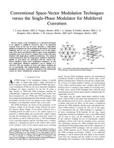
Table 1 shows summaries of state vectors and the duty cycles in the three regions in the complex plane d-q. Finally, in order to validate the explained technique, experimental results obtained in a 50kW back-to-back NPC three-level converter prototype, show a satisfactorily good performance of the proposed algorithm. In these figures, the phase voltage, the phase-phase voltage, and the neutral-phase voltage are illustrated.
Figure 7: Origin of the sub-cube where the reference vector is supposed to be found.
702
703
2.3
Three-dimensional space vector algorithm of multilevel converters
Finally, a three-dimensional (3D) space vector algorithm of multilevel converters for compensating harmonics and zero sequence in three phase four wire systems with neutral is presented in this section. The low computational cost of the proposed method is always the same and it is independent of the number of levels of the converter. The conventional two-dimensional space vector algorithms represent a particular case of the proposed generalized modulation algorithm. In general, the presented algorithm is useful in systems with or without neutral, unbalanced load, triple harmonics, and for generating whatever 3D control vector. The algorithm presented in this work is a generalization of the well known 2D space vector technique, including the algorithms explained above [16]. The replacement of conventional two level converters by multilevel converters in active filters highly improves the harmonic content of the output signal of the converter. Most of the active filter control techniques found in the bibliography are based on current control pulse width modulation (PWM) or bang-bang [15], where each leg of the converter is independently controlled. However, it would be desirable to use an effective 3D Space Vector Modulation for this kind of applications because it can drastically reduce the control complexity and the computational load. It is necessary to develop a new 3D space vector algorithm for multilevel converters to compensate a zero sequence in active power filters with neutral with single-phase distorting loads, which generate large neutral currents. In general, the proposed algorithm is useful in systems with or without neutral, unbalanced load, triple harmonics and for generating whatever 3D control vector. The space vectors will coplanar if the system is balanced without triple harmonics. However, it is necessary to generalize the approach to a 3D space if the system is unbalanced or if there is zero sequence or triple harmonics because the reference vectors are not on a plane. The proposed algorithm is the first 3D space vector modulation technique for multilevel converters which permits the on-line calculation of the sequence of the nearest space vector for generating the reference voltage vector [16,18]. This generalized method provides the nearest switching vectors sequence to the reference vector and calculates the on-state durations of the respective switching state vectors without involving trigonometric functions, look-up tables, or coordinate system transformations which increase the computational load corresponding to the modulation of multilevel con704
verters. In this work, a very simple and fast 3D modulation algorithm based on geometrical considerations is presented. The computational cost of the proposed method is very low and independent of the number of levels of the converter. This technique can be used as modulation algorithm in all applications which provide a 3D vector control. 2.3.1
Reference vector synthesis
During each modulation subcycle of duration Tm , a switching sequence is generated. It is composed of four switching state vectors u1 (t1 ), u2 (t2 ), u3 (t3 ), and u4 (t4 ), where t1 , t2 , t3 , and t4 are the on-state durations of the active switching state vectors. The four vectors nearest to the reference vector must be identified [18]. The proposed 3D Space Vector Modulation (SVM) algorithm easily calculates the four state vectors which generate the reference vector. In general, with unbalanced systems or with triple harmonics, the reference vector could be not placed in the 2D plane of the multilevel converter. In this way, it is necessary to use a switching sequence with four state vectors. Thus, the reference vector will be pointing to a volume which is a tetrahedron. The vertices of that tetrahedron are the state vectors of the switching sequence. In addition, the algorithm permits to obtain the corresponding duty cycles without using tables or trigonometric functions. The modulation algorithm input is the normalized voltage vector. The normalization only depends on the number of levels of the multilevel converter n, and the voltage level value of the DC-link capacitors, VDC [16]. The q reference vector must be multiplying by the normalization constant 2 VDC 3 n−1 .
Step 1: Find the sub-cube where the reference vector is pointing to. The space vectors of a multilevel converter form a cube in a 3D space. This space can be decomposed into several tetrahedrons which generate the cube total volume. For a certain reference vector in three-phase coordinates (ua , ub , uc ), the integer part of each component (a, b, c) is calculated, where a=
integer (ua ),
b=
integer (ub ),
c=
integer (uc ).
(20)
The 3D space is formed by a certain number of sub-cubes depending on the number of the levels of the converter. (a, b, c) are the origin coordinates 705
Figure 8: Tetrahedrons into the cube with the corresponding state vectors.
706
corresponding to the reference system of the sub-cube where the reference vector is pointing to. Step 2: Six tetrahedrons are considered into each sub-cube. Therefore, it is necessary to define the tetrahedron where the reference vector is pointing to. This tetrahedron is easily found by comparing with three planes into the 3D space which define the six tetrahedrons inside the sub-cube. The three planes which define the six tetrahedrons are shown in [16,18]. Only the maximum of three comparisons is needed. Step 3: Once (a, b, c) coordinates are known, the main step of the algorithm consists in calculating the four space vectors corresponding to the four vertices of a tetrahedron into the selected sub-cube (in step 1). These vectors will generate the reference vector. Configurations of the 3D space with different number of tetrahedrons into the cube have been studied. However, the minimum number of comparisons is obtained using six tetrahedrons [16,18]. In Fig. 8, the tetrahedrons in the cube with the corresponding state vectors are illustrated.
Figure 9: Algorithm for the selection of each tetrahedron with the corresponding state vectors. 707
Figure 10: Experimental results obtained in a 50kW back-to-back NPC three-level converter prototype: a) phase voltage; b) phase-phase voltage; c) neutral-phase voltage.
708
Step 4: Calculation of the switching times. The new algorithm calculates on-line the four state vectors in the 3D space and the corresponding duty-cycles using only sixty nine instructions and a maximum of three comparisons for calculating the suitable tetrahedron. The computational load is always the same and is independent of the number of levels of the multilevel converter. In addition, the algorithm provides the switching sequence that minimizes the total harmonic distortion and the commutation number of the semiconductor devices. General structure of the algorithm The flow diagram of the new 3D modulation algorithm for choosing the tetrahedron where the reference vector is pointing to is shown in Fig. 9. Notice that the algorithm is extremely simple. 2.3.2
Calculation of duty-cycles
Once the state vectors which generate each reference vector are known, the corresponding duty-cycles are calculated. The algorithm generates a matrix with four state vectors and the corresponding switching times ti . 1 1 1 Sa Sb Sc d1 Sa2 S 2 Sc2 d2 b S= Sa3 S 3 Sc3 d3 b (21) Sa4 Sb4 Sc4 d4 ti = di Tm , i = 1, ..., 4 where Tm is the sample time. The state vectors are the vertices of the corresponding tetrahedron which generates the reference vector. The equations to be solved are: ua = Sa1 d1 + Sa2 d2 + Sa3 d3 + Sa4 d4, ub = Sb1 d1 + Sb2 d2 + Sb3 d3 + Sb4 d4, (22) uc = Sc1 d1 + Sc2 d2 + Sc3 d3 + Sb4 d4, d1 + d2 + d3 + d4 = 1. The numeric evaluation of the duty cycles or on-state durations of the switching states are reduced to a simple addition as shown in Table 2. a, b, and c represent the different voltage levels of the capacitors battery. They
709
acquire values between zero and n − 1 where n is the number of levels of the multilevel converter. The duty cycles are functions only of the reference vector components and the integer part of reference vector coordinates. In addition, the optimized switching sequence is selected in order to minimize the switching number. The space vectors sequence in half cycle is: u1 = (Sa1 , Sb1 , Sc1 ), u2 = (Sa2 , Sb2 , Sc2 ), u3 = (Sa3 , Sb3 , Sc3 ), and u4 = (Sa4 , Sb4 , Sc4 ). In the second half cycle the space vectors form a reverse sequence. Tetrahedron Case 1.1
Case 1.2
Case 1.3
Case 2.1
Case 2.2
Case 2.3
Space vectors sequence (S1a , S1b , S1c ) = (a, b, c) (S2a , S2b , S2c ) = (a + 1, b, c) (S3a , S3b , S3c ) = (a + 1, b, c + 1) (S4a , S4b , S4c ) = (a + 1, b + 1, c + 1) (S1a , S1b , S1c ) = (a, b, c) (S2a , S2b , S2c ) = (a, b, c + 1) (S3a , S3b , S3c ) = (a + 1, b, c + 1) (S4a , S4b , S4c ) = (a + 1, b + 1, c + 1) (S1a , S1b , S1c ) = (a, b, c) (S2a , S2b , S2c ) = (a, b, c + 1) (S3a , S3b , S3c ) = (a, b + 1, c + 1) (S4a , S4b , S4c ) = (a + 1, b + 1, c + 1) (S1a , S1b , S1c ) = (a, b, c) (S2a , S2b , S2c ) = (a, b + 1, c) (S3a , S3b , S3c ) = (a, b + 1, c + 1) (S4a , S4b , S4c ) = (a + 1, b + 1, c + 1) (S1a , S1b , S1c ) = (a, b, c) (S2a , S2b , S2c ) = (a, b + 1, c) (S3a , S3b , S3c ) = (a + 1, b + 1, c) (S4a , S4b , S4c ) = (a + 1, b + 1, c + 1) (S1a , S1b , S1c ) = (a, b, c) (S2a , S2b , S2c ) = (a + 1, b, c) (S3a , S3b , S3c ) = (a + 1, b + 1, c) (S4a , S4b , S4c ) = (a + 1, b + 1, c + 1)
Switching times d1 = 1 + a — ua , d2 = -a + c + ua — uc , d3 = b — c — ub + uc , d4 = - b + ub , d1 = 1 + c - uc , d2 = a — c — ua + uc , d3 = - a + b + ua - ub , d4 = - b + ub , d1 = 1+ c - uc , d2 = b — c — ub + uc , d3 = a — b — ua + ub , d4 = - a + ua , d1 = 1 + b — ub , d2 = - b + c + ub — uc , d3 = a - c — ua + uc , d4 = - a + ua , d1 = 1 + b - ub , d2 = a — b —ua + ub , d3 = - a + c + ua -uc , d4 = - c + uc , d1 = 1 + a - ua , d2 = - a + b + ua - ub , d3 = - b + c + ub - uc , d4 = - c + uc .
Table 2. States sequence and switching times.
710
The proposed 3D technique is a generalization of the 2D space vector algorithms. One should notice the behaviour of a balanced system without triple harmonics using the 3D algorithm. In this case, one of the four active vectors given by the algorithm has the switching time equal to zero. Then, the problem is reduced to the well known 2D situation. The algorithm has been successfully implemented with a micro controller in order to prove the technique using a reference vector with triple harmonics and zero sequence. The modulation is the output signal of the micro controller which has been digitally filtered with a low pass filter that eliminates the higher frequencies. In this way, this permits to obtain the output signals of Diode Clamped Inverter (Va , Vb , and Vc ) obtaining signals that follow the input reference signals.
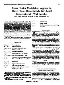
Figure 11: Comparison of computational burden.
711
Finally, the comparison between the proposed modulation algorithms and a SVM with very low computational burden found in the literature [17], is illustrated in Fig. 11. This figure shows that the complexity of the algorithms and the number of instructions using the proposed methods are drastically reduced compared with other conventional Space Vector Modulation (SVM) and sinusoidal PWM modulation techniques.
3
Conclusions
Three new space vector modulation techniques for multilevel converters are explained in this survey. These algorithms are very useful for the on-line computation of the switching sequence and the on-state durations of the respective switching state vectors corresponding to the modulation of multilevel converters without physical affecting the connected load. The vector selection is adjusted according to the input reference to improve the voltage generation being balanced the DC-link capacitor voltage. These techniques permit an economic and simple electronic implementation and the on-line computation of the switching state vectors for the modulation of a multilevel inverter. Moreover, the space vector modulations present the advantage of eliminating the angle from the calculations and the numeric evaluation of the on-state durations are reduced to a simple addition. The computational burden, the complexity of the algorithms and the number of instructions using the proposed methods are drastically reduced compared with other conventional Space Vector Modulation (SVM) and sinusoidal PWM modulation techniques. The 3D space vector modulation algorithm, explained in the last section of this paper, directly allows compensating zero sequence in systems with a neutral and optimizing the switching sequence minimizing the number of switching. The computational complexity is very low and independent of the number of levels of the converter. This algorithm does not use trigonometric functions or look-up tables. It has been satisfactorily implemented in very low-cost micro controllers. This technique can be used as a modulation algorithm in all applications needing a 3D control vector such as active filters with four wires with single-phase distorting loads which generate large neutral currents, where the conventional 2D space vector modulations cannot be used. This work was supported by the Comisión Interministerial de Ciencia y Tecnología of the Spanish government under Project DPI 2001-3089.
712
References [1] M. Veenstra and A. Rufer, IEEE Power Electronics Specialists Conference, PESC’2000, v. 3, p.1387 (2000). [2] A. Nabae, I. Takahashi, and H. Akagy, IEEE Trans. on Industrial Applications 17, 518 (1981). [3] L.M. Tolbert and T.G. Habetler, IEEE Trans. on Industrial Applications 35, 1098 (1999). [4] R. Rojas, T. Onhishi, and T. Suzuki, IEE Proc. on Electric Power Applications 142, 390 (1995). [5] N. Celanovic and D. Boroyevich, IEEE Trans. on Industry Applications 37, 637 (2001). [6] O. Alonso, L. Marroyo, and P. Sanchis, Proc. 10-th European Conference on Power Electronics and Applications, EPE’2001 (2001). [7] M.M. Prats, J.M. Carrasco, and L.G. Franquelo, Proc. PCIM’2002 (Nurenberg, Germany, 2002). [8] M.M. Prats, J.M. Carrasco, and L.G. Franquelo, IEE Electronics Letters 38, 1398 (2002). [9] R. Teodorescu, F. Blaabjerg, J.K. Pedersen, E. Cengelci, and P.N. Enjeti, IEEE Trans. on Industrial Electronics 49, 832 (2002). [10] B.M. Song, S. Gurol, C.Y. Jeong, D.W. Yoo, and J.S. Lai, Proc. Industry Applications Conference, IAS’01, p.1461 (2001). [11] N. Celanovic and D. Boroyevich, IEEE Trans. on Power Electronics 15, 242 (2000). [12] J.-O. Krah and J. Holtz, IEEE Trans. on Industry Applications 35, 1039 (1999). [13] M.M.Prats, J.M. Carrasco, and L.G. Franquelo, IEE Electronics Letters 38, 1398 (2002). [14] M.M. Prats, J.I. León, R.Portillo, J.M. Carrasco, and L.G. Franquelo, Journal of Circuits, Systems and Computers 13. 845 (2004).
713
[15] S. Buso, L. Malesani, and P. Mattavelli, IEEE Trans. on Industrial Electronics 45, 722 (1998). [16] M.M. Prats, L.G. Franquelo, J.I. León, R. Portillo, E. Galvan, and J.M. Carrasco, IEEE Power Electronics Letters 1, 104 (2003). [17] Dengming Peng, F.C. Lee, and D. Boroyevich, IEEE Power Electronics Specialists Conference PESC’02, v.2, p.509 (2002). [18] M.M. Prats, PhD thesis (tesis doctoral), “Nuevas técnicas de modulación vectorial para convertidores electrónicos de potencia multinivel”, Department of Electronic Engineering of the University of Seville, Spain (2003).
714