Using PHP format - The GENE Code

PHYSICS OF PLASMAS

VOLUME 7, NUMBER 5

MAY 2000

Electron temperature gradient driven turbulence* F. Jenko,† W. Dorland,a) M. Kotschenreuther,b) and B. N. Rogersa) Max-Planck-Institut fu¨r Plasmaphysik, EURATOM Association, 85748 Garching, Germany

共Received 19 November 1999; accepted 4 February 2000兲 Collisionless electron-temperature-gradient-driven 共ETG兲 turbulence in toroidal geometry is studied via nonlinear numerical simulations. To this aim, two massively parallel, fully gyrokinetic Vlasov codes are used, both including electromagnetic effects. Somewhat surprisingly, and unlike in the analogous case of ion-temperature-gradient-driven 共ITG兲 turbulence, we find that the turbulent electron heat flux is significantly underpredicted by simple mixing length estimates in a certain parameter regime (sˆ ⬃1, low ␣兲. This observation is directly linked to the presence of radially highly elongated vortices 共‘‘streamers’’兲 which lead to very effective cross-field transport. The simulations therefore indicate that ETG turbulence is likely to be relevant to magnetic confinement fusion experiments. © 2000 American Institute of Physics. 关S1070-664X共00兲95905-6兴

I. INTRODUCTION

However, there are other potential stabilization mechanisms such as negative magnetic shear or electromagnetic effects which can stabilize the ETG modes and lead to an electron ITB. Results like these call for nonlinear numerical simulations of ETG turbulence in order to quantify its experimental relevance, and to test the above ideas. In Sec. II, we give a brief review of earlier ETG studies including quasilinear estimates of the electron heat transport caused by electromagnetic ETG modes as well as nonlinear, two-dimensional fluid simulations of ETG turbulence. Both lines of work indicate that the turbulent electron heat transport might be significantly underpredicted by simple mixing length estimates. In Sec. III we give a brief description of the model equations and the numerical techniques used to solve them. Moreover, nonlinear simulation results are presented which highlight the importance of radially highly elongated vortices 共‘‘streamers’’兲 in a certain parameter regime (sˆ ⬃1, low ␣兲. In Sec. IV, we discuss these results with respect to the linear behavior and nonlinear generation of poloidal shear flows 共‘‘zonal flows’’兲 as well as the breakup of streamers due to Kelvin–Helmholtz physics. In Sec. V, we summarize and comment upon open questions left for future work.

As is well known, the cross-field particle and heat transport in magnetically confined fusion plasmas generally exceeds neoclassical predictions by up to two orders of magnitude. There is strong experimental evidence that these anomalous confinement properties can be attributed to various kinds of small-scale turbulence driven by density or temperature gradients. Currently it is widely thought that two types of instabilities are sufficient to explain the anomalous transport in the core region of tokamak plasmas, i.e., iontemperature-gradient-driven 共ITG兲 modes and trappedelectron modes. Recent experiments seem to indicate, however, that this basic picture is incomplete. Among them are observations by Stallard et al.1 in DIII-D tokamak plasmas with an internal transport barrier 共ITB兲. They find that within the ITB, ion thermal transport can be reduced to the neoclassical level. Furthermore the region of reduced ion heat transITG where port is well characterized by the condition ␥ E ⬎ ␥ max ITG ␥ E is the measured EÃB flow shearing rate, and ␥ max is the calculated maximum linear growth rate for ITG modes in the absence of flow shear. At the same time, the electron thermal transport hardly changes 共except for discharges with large negative magnetic shear兲, and the observed electron temperature gradient within the ITB is close to the critical value provided by the linear theory of electron-temperaturegradient-driven 共ETG兲 modes. Similar observations were reported from the Tokamak Fusion Test Reactor 共TFTR兲.2 These findings support the hypothesis2,3 that within an ITB, ITG turbulence is suppressed by EÃB shear flow, whereas ETG turbulence controls the electron thermal transport. Due to their smaller spatial scales and larger linear growth rates, ETG modes are not strongly affected by the shear flow and therefore set a lower limit on the electron heat diffusivity ␹ e .

II. BRIEF REVIEW

ETG modes are collisionless microinstabilities driven by electron temperature gradients and basically electrostatic in nature. Their linear dynamics have been studied by various authors4–8 and 共in the electrostatic and adiabatic limit兲 bear strong resemblance to those of ITG modes, with the roles of electrons and ions reversed. At typical perpendicular wavelengths ␳ e ⱗ␭⬜ Ⰶ ␳ i and frequencies ␻ ⬃ v te /L n , toroidal ETG modes are linearly unstable when R/L T e exceeds a critical value.8 Here, ␳ e and ␳ i are, respectively, the electron and ion gyroradii, v te is the electron thermal speed, L n and L T e are, respectively, the background density and electron temperature scale lengths, and R is the major radius. This instability criterion can be reformulated in terms of a critical ␩ e ⫽L n /L T e if the density gradient is sufficiently steep. 共This is

*Paper FI16 Bull. Am. Phys. Soc. 44, 91 共1999兲. † Invited speaker. a兲 Institute for Plasma Research, University of Maryland, College Park, Maryland 20742. b兲 Institute for Fusion Studies, The University of Texas, Austin, Texas 78712. 1070-664X/2000/7(5)/1904/7/$17.00

1904

© 2000 American Institute of Physics

Phys. Plasmas, Vol. 7, No. 5, May 2000

why ETG modes are sometimes called ␩ e modes.兲 Because of k⬜ ␳ i Ⰷ1 the ion response is almost adiabatic. Consequently, ETG modes do not drive significant ion thermal, momentum, or particle transport. Assuming a perfect isomorphism between ITG and ETG turbulence3 in a deuterium plasma, the ETG ␹ e ⬃ ␳ 2e v te /L n ⬅D ETG is smaller than the ITG ␹ i ⬃ ␳ 2i v ti /L n by a factor of 60 for comparable deviations from criticality. It was found experimentally1,2 that within an ITB, L T e is very close to L Tcrit . This result is difficult to reconcile with the isomorphic e

model since the ␹ e that one obtains from ETG modes by analogy with ITG modes is too small 共particularly for the higher-field TFTR discharges兲 to enforce marginality of L T e . However, a central result of this paper is that there are important differences in the nonlinear dynamics of ETG and ITG modes which break this isomorphism. Relaxing the electrostatic and adiabatic assumptions leads to further differences. An interesting development was triggered in 1978 by Ohkawa9 共see, e.g., Refs. 10–12兲. General considerations of electron dynamics along perturbed magnetic field lines led him to describe the anomalous electron heat transport by the formula ␹ e ⬃ ␦ s2 ␯ te ⬅D * , where ␦ s ⫽c/ ␻ pe is the collisionless skin depth, ␯ te ⫽ v te /qR is the electron transit frequency, and q is the safety factor. Because of D * ⬃D ETG/ ␤ , Ohkawa’s prediction for ␹ e matches the experimentally observed transport levels much better than the naive ETG estimate, ␹ e ⬃D ETG. Subsequently, it was proposed that various collisionless electromagnetic microinstabilities could be the source of the magnetic fluctuations underlying Ohkawa’s formula.13–17 Particularly, it was shown that quasilinear estimates for the turbulent transport due to collisionless electromagnetic ETG modes yield scalings very similar to Okhawa’s result.7,8,18 Physically, it was argued that ETG electron heat transport is dominantly by magnetic flutter. Early nonlinear simulations of ETG modes suggested that a different physical process might be more important. An electromagnetic Braginskii fluid model in twodimensional unsheared slab geometry exhibited turbulent vortices with high elongation in the radial direction.19 These ‘‘streamers’’ were found to produce EÃB transport which greatly exceeded the quasilinear estimates. General considerations of temperature-gradient-driven turbulence by Cowley et al. show that such elongated eddies are the most unstable and have the highest saturation amplitudes, even in the presence of magnetic shear.20 They further argue that the saturation of streamers is controlled by the nonlinear evolution of secondary instabilities. A deeper understanding of ETG turbulence clearly requires nonlinear electromagnetic simulations. The ETG ␹ e that we find is dominated by streamer EÃB convection and turns out to be much larger than the isomorphic expectations, and in fact large enough to be experimentally relevant, particularly for the cases of Refs. 1 and 2.

Electron temperature gradient driven turbulence

1905

III. NONLINEAR GYROKINETIC SIMULATIONS A. Model equations and numerical techniques

Our simulations are based on the electromagnetic nonlinear gyrokinetic equation.21–25 This equation describes the evolution of fluctuations which satisfy ˜h ˜ ˜A 储 ˜B 储 ␻ ␳ e␾ ⬃ ⬃ ⬃ ⬃ ⬃ Ⰶ1, F0 T B␳ B ⍀ L

k 储 L⬃k⬜ ␳ ⬃1, 共1兲

where ˜h is the nonadiabatic part of the perturbed distribution ˜ and function, F 0 is the equilibrium distribution function, ␾ ˜A 储 are the perturbed parts of the electrostatic and parallel vector potential, ˜B 储 is the perturbed parallel magnetic field, B is the equilibrium magnetic field, L is an equilibrium scale length 共of density, temperature, or magnetic field兲, and ⍀ ⫽eB/(mc) and ␳ ⫽ v t /⍀ are the cyclotron frequency and thermal gyroradius of a given particle species with thermal velocity v 2t ⫽T/m and charge e. The simulations are performed in field-line-following coordinates using toroidal flux tubes.20,26,27 In such coordinates, the nonlinear gyrokinetic equation may be written as

冉

冊 冉

冊

d ⳵ ⳵F0 ⫹ v 储 b•“⫹i ␻ d ˜h ⫹ ⫺i ␻ T e ˜␹ ⫽0. * dt ⳵t ⳵⑀

共2兲

Here, the distribution function F 0 ⫽F 0 ( ⑀ ,⌿) depends only on the energy ⑀ ⫽m v 2 /2 and the flux surface label ⌿, where ⌿ is the equilibrium poloidal magnetic flux enclosed by the magnetic surface of interest. The total time derivative is given by d t ⫽ ⳵ t ⫹(c/B) 关 ˜␹ ,• 兴 , where 关 •,• 兴 is the Poisson bracket. The perpendicular curvature and “B drifts are given by ␻ d ⫽k⬜ •BÃ(m v 2储 b•“b⫹ ␮ “B)/(Bm⍀), where ␮ ⫽m v⬜2 /(2B) and the fields are represented by

冉

˜⫺ ˜␹ ⫽J 0 共 ␥ 兲 ␾

冊

J 共 ␥ 兲 m v⬜2 ˜B 储 v储 ˜A 储 ⫹ 1 . c ␥ e B

共3兲

Here, ␥ ⫽k⬜ v⬜ /⍀ and ␻ T ⫽n 0 c ⳵ ⌿ F 0 , where n 0 is the tor* oidal mode number of the perturbation. The self-consistent electromagnetic field fluctuations are computed from the gyrokinetic Poisson–Ampe`re equations,

冋

˜ ⫽4 ␲ ⵜ⬜2 ␾

兺s e 冕 dv e ␾˜

ⵜ⬜2 ˜A 储 ⫽⫺

4␲ c

˜B 储 4␲ ⫽⫺ 2 B B

兺s

兺s

冕

冕

册

⳵F0 ⫹J 0 共 ␥ 兲˜h , ⳵⑀

共4兲

dve v 储 J 0 共 ␥ 兲˜h ,

共5兲

J 1共 ␥ 兲 ˜h . ␥

共6兲

dvm v⬜2

The Bessel functions J 0 and J 1 arise because Eqs. 共4–6兲 are formulated in particle space x, rather than in gyrocenter ˜ in Poisspace R. We retain the Debye-shielding term ⵜ⬜2 ␾ son’s equation, since the electron Debye length ␭ De can be comparable to ␳ e in laboratory fusion experiments. However, we find that space charge physics has a significant effect on the simulation results only for ␭ De Ⰷ ␳ e which is not satisfied under typical tokamak conditions.

1906

Jenko et al.

Phys. Plasmas, Vol. 7, No. 5, May 2000

We present simulation results from two independent parallel codes, each based on the equations above, and each employing a fixed grid in five-dimensional phase space. Both codes include velocity–space collision operators which were not used in this study. The first code 共Gyrokinetic Electromagnetic Numerical Experiment, GENE兲 uses explicit finitedifference methods of the upwind and predictor–corrector type. The code is second-order accurate in phase space and time, and shows excellent parallel performance. The algorithm and parallelization strategy are similar to those used in the drift-kinetic Vlasov code described in Ref. 28. A linear combination of ˜h and ˜␹ is advanced, to avoid difficulties associated with the time derivative on the right-hand side 共RHS兲 of Eq. 共2兲. The linear terms are treated by a Lax– Wendroff scheme,29 whereas the nonlinear advection term is computed according to a multidimensional upwind method.30 Trapped particles and ˜B 储 fluctuations are neglected in the GENE simulations presented below. F 0 is chosen to be a Maxwellian depending 共weakly兲 on the background density and electron temperature, and as magnetic geometry we take the sˆ -␣ model magnetohydrodynamic MHD equilibrium.31 The second code is GS2, a nonlinear generalization of a widely used gyrokinetic stability code.32 An operator splitting scheme is used, so that the linear terms 关including Eqs. 共4兲–共6兲兴 may be treated implicitly. The nonlinear terms are evaluated with a dealiased pseudospectral algorithm in the plane perpendicular to the field line. A second-order Adams– Bashforth scheme is used to advance the nonlinear terms in time. Nonuniform coordinate meshes are used in velocity space to improve the resolution, particularly for the trapped– passing boundary. A small amount of upwind diffusion is typically used, only in the direction along the field line. In the absence of upwind diffusion, the algorithm is secondorder accurate in space and time. Good parallel performance is achieved by employing multiple-domain decomposition in four of the five dimensions at all times. In both codes, the Bessel functions 共which represent the gyroaverages兲 are evaluated in Fourier space. This guarantees the applicability of the algorithms to arbitrary perpendicular length scales. This feature is very important for ETG computations that include ion dynamics. However, unless stated otherwise, the ion response is assumed to be purely adiabatic. This assumption is reasonable as long as k⬜ ␳ i Ⰷ1, which is satisfied for realistic electron–ion mass ratios in simulations carried out in flux tubes with perpendicular dimensions L x ,L y ⱗ ␳ i . Typically we use 1–3 ␳ e per grid cell, 16–32 grid points per 2␲ along the parallel direction, 50⫻10 points in velocity space, and up to 105 time steps which are dynamically adjusted in both codes. We normalize the perpendicular spatial scales to ␳ e , the parallel spatial scales to L n , and the time to L n / v te . The fluctuating quantities are normalized by the appropriate equilibrium values, with an additional scale factor that reflects the fundamental ordering. For example, the normalized fluc˜ /T e ) tuating potential and density are defined by ( 兩 e 兩 ␾ ˜ /n)(L n / ␳ ). Conventional mixing-length ar⫻(L n / ␳ ) and (n guments predict that the normalized, steady-state turbulent fluctuations should be of order unity. In this case, the turbu-

FIG. 1. The density response of the flux-surface averaged component affects transport strongly. The upper curve has n⬀ ␾ , and the lower curve has n ⬀( ␾ ⫺ 具 ␾ 典 ).

lent transport would be of order ␹ e ⬃D ETG, and ␹ e ⬃(m e /m i ) 1/2 ␹ i Ⰶ ␹ i ⬃ ␳ 2i v ti /L n . Thus, if ETG and ITG turbulence co-existed and were fully analogous, ␹ e from ETG could probably be neglected for most magnetic confinement fusion plasmas. B. Nonlinear simulation results

In the presence of electric and perpendicular magnetic field fluctuations, the turbulent electron heat flux in the radial direction 共denoted by x兲 is given by Q⫽

冓冓 冕 me 2

dv共 v Ex ⫹ v 储 b x 兲v 2˜f e

冔冔

,

共7兲

˜ ⫹eJ 0 ␾ ˜ ⳵ ⑀ F 0 . There is an ‘‘electrostatic’’ comwhere ˜f ⫽h ponent due to EÃB convection and an ‘‘electromagnetic’’ component due to magnetic flutter. Here, the double angular braces denote averaging over the entire simulation volume. We have performed a few sheared-slab ETG simulations, with electrostatic gyrofluid 共GRYFFIN兲33 and electromagnetic drift-kinetic28 codes. In this case, we find a typical 共predominantly electrostatic兲 transport level of ␹ e ⬃D ETG. The toroidal simulations are more interesting. In the electrostatic limit, the equations describing ETG and ITG modes are the same 共with the electron and ion roles reversed兲, except for one term: the ion response in ETG modes is purely adiabatic (n⬀ ␾ ), while the electron response in ITG modes is adiabatic with a vanishing fluxsurface averaged component 关 n⬀( ␾ ⫺ 具 ␾ 典 ) 兴 . 33,34 The purely adiabatic ion response in ETG modes inhibits saturation and allows higher transport. Figure 1 shows the magnitude of this effect, by comparing two GS2 simulations in which only the form of the response of the adiabatic species is changed. Pictured is the heat flux Q 关in units of (nT/L n ) ␳ 2 v t /L n 兴 versus time. The parameters are q⫽1.4, sˆ ⫽0.8, R/L T ⫽6.9, R/L n ⫽2.2, T i ⫽T e , Z eff⫽1, ␤ ⫽0 共electrostatic兲, and minor radius r/R⫽0.18 共trapped particles兲. The simulation domain had L x ⫽2L y ⫽100␳ , with N x ⫽2N y ⫽54 gridpoints in the perpendicular directions, and 32 gridpoints along the field line. The average value of the lower curve corresponds to ␹ ⫽2.5␳ 2 v t /L n , which is in good agreement with established gyrokinetic particle simulations.35 The larger transport indicated by the upper curve motivates the present study.

Phys. Plasmas, Vol. 7, No. 5, May 2000

Electron temperature gradient driven turbulence

1907

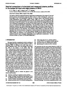
˜ contours in the outboard x-y plane. This snapshot FIG. 4. Characteristic ␾ was taken at t⫽180 of the run shown in Fig. 2. Positive and negative fluctuations are drawn, respectively, with solid and dashed lines. FIG. 2. Heat flux for an electromagnetic, single-species ETG simulation employing a radially elongated simulation box with L x ⫽4 L y ⫽256 ␳ e .

In Fig. 2, electromagnetic ETG results from GENE are shown. The parameters are the same as in Fig. 1, except ␣ ⫽0.45 共␤ is chosen accordingly兲. The simulation domain is larger (L x ⫽4L y ⫽256␳ e ) and better resolved (⌬x⫽⌬y ⫽ ␳ e ). The steady-state transport corresponds to ␹ e ⬃60 D ETG. For both GENE and GS2, choosing L x ⫽L y in single-species runs results in nonsaturating streamer transport for typical tokamak parameters. This effect is explained in Sec. IV, where we identify the physical saturation mechanisms. Of course, the real ion response is not exactly adiabatic, and the departure from adiabaticity is expected to be important. The turbulent electron heat flux for a two-species run from GENE is shown in Fig. 3. The physics parameters are the same as in Fig. 2, except nonadiabatic ions with m i /m e ⫽1000 are included, and the box dimensions are increased to L x ⫽L y ⫽400 ␳ e with ⌬x⫽⌬y⫽3 ␳ e . The ion temperature gradient was R/L T i ⫽0.55, which is below the ITG critical gradient. With nonadiabatic ions, we find saturating turbulence even with L x /L y ⫽1 if wavenumbers smaller than k⬜ ␳ i ⬃1 are included. The resulting electron heat and particle transport is characterized by ␹ e ⬃60 D ETG and D/ ␹ e ⬃0.005. ˜ contours in the outFigure 4, showing characteristic ␾ board x-y plane at t⫽180 of the run shown in Fig. 2, reveals that the high transport levels are associated with streamers. These radial flows are potentially able to transport plasma up and down the temperature gradient very effectively. To actually be effective, however, there must be a phase shift between potential and temperature fluctuations. Figure 5 shows the probability distribution P(k y , ␣ p ) for the k y components

FIG. 3. Heat flux for an electromagnetic, two-species ETG simulation. The physics parameters are the same as in Fig. 2 except for a mass ration of m i /m e ⫽1000.

of ␾ and T e fluctuations having a given relative phase ␣ p 苸 关 ⫺ ␲ , ␲ 兴 . The maximum of P(k y , ␣ p ) occurs for modes with k y ⬃0.2 and ␣ p ⬃ ␲ /3, yielding a large heat transport in the radial direction. We also investigated the behavior of Q in sˆ -␣ space holding the other physical parameters constant at q⫽1.4, L n /R⫽0.45, L T e /R⫽0.15, and T e /T i ⫽1. The qualitative results from more than 20 single-species simulations with the GENE code are summarized in Fig. 6. 共Note that because ␣ ⫽⫺q2R␤⬘ is proportional to ␤, we varied both parameters simultaneously.兲 Generally, one observes that for high ␣ and low sˆ the transport is reduced to low levels (Q⬃20) and that streamers are absent. This corresponds to plasma parameters characteristic of ITB’s in ‘‘advanced’’ tokamaks, and of high confinement mode 共H-mode兲 pedestals 共particularly if bootstrap currents are taken into account36兲. Interestingly, the transition region between these two regimes is relatively narrow; e.g., a change of ␣ by some 10% can cause a large change in the transport. For points within the transition region, the transport exhibits bursty behavior. The dependence of Q on these parameters is also seen with GS2. To evaluate the impact of different finite-␤ effects on the ETG system, we repeated the run shown in Fig. 2, keeping Shafranov shift modifications of the magnetic geometry but neglecting electromagnetic effects on the dynamics. In this case, we obtained a much lower transport level. Switching off only the nonlinear magnetic flutter terms was also stabilizing. These results indicate that Fig. 6 cannot be explained in terms of geometry effects alone. 关Our results are consistent with the idea that magnetic flutter nonlinearities 共stresses兲 tend to suppress the secondary Kelvin–Helmholtz

FIG. 5. Probability distribution P(k y , ␣ p ) for the k y components of ␾ and T e fluctuations having a given relative phase ␣ p 苸 关 ⫺ ␲ , ␲ 兴 . The dominant modes have k y ⬃0.2 and ␣ p ⬃ ␲ /3.

1908

Phys. Plasmas, Vol. 7, No. 5, May 2000

FIG. 6. Qualitative behavior of Q in sˆ -␣ space as observed in more than 20 numerical simulations 共denoted by the symbol 丣 兲. The physical parameters were q⫽1.4, L n /R⫽0.45, L T e /R⫽0.15, and T e /T i ⫽1.

instability37 共discussed in Sec. IV A兲.兴 It is crucial to note here that for all our runs performed in the low-beta regime ( ␤ ⱗ10%) the electron heat flux is essentially electrostatic. This is found even when the peak of the fluctuation spectrum lies close to k⬜ ␦ s . The quasilinear calculations mentioned in Sec. II therefore do not explain our nonlinear simulation results. IV. DISCUSSION

There are five significant differences between ITG and ETG turbulence. 共1兲 The responses of the ITG electrons and ETG ions differ. 共2兲 Zonal flow physics differs because shielding of 共turbulent兲 sources varies strongly with radial wavenumber. 共3兲 Magnetic flutter physics differs because of the disparate velocities of electrons and ions along the field lines. 共4兲 Magnetic well physics differs because the disparity in gyroradii allows self-dug wells at short wavelengths. 共5兲 ETG instabilities can themselves be driven unstable by perturbed radial electron temperature gradients which might arise from longer-wavelength turbulence. Less significant differences include the role of Debye-scale physics. Conclusive results regarding item 共5兲 require computational resources that should become available within a year or two. While we have not investigated the difference in the magnetic well physics 关item 共4兲兴 numerically, this difference is not difficult to appreciate. For k⬜ ␳ i Ⰷ1, the ion contribution to the RHS of Eq. 共6兲 is neglible. As a result, the com˜ fails to probination of ␻ T ˜B 储 and the term ⬀ ␮ bÓB•“h * duce pure curvature in the vorticity equation 关which can be derived from Eq. 共2兲兴, and thus magnetic wells associated with the ion pressure gradient can help stabilize shortwavelength instabilities such as the ETG mode. Item 共3兲 has not been explored adequately in the long-wavelength 共ITG兲 limit, so that comparisons of ITG and ETG magnetic flutter physics would be premature. Nevertheless, we note that our results in this regard are consistent with Ref. 37. The most significant effects are items 共1兲 and 共2兲, to which we now turn. A. Streamer breakup

We find that the most important nonlinear process in the electrostatic toroidal simulations 共for typical parameters兲 is the secondary Kelvin–Helmholtz 共KH兲 instability which is

Jenko et al.

driven by the shear in the poloidal electric field of a streamer. Other secondary instabilities appear to be stabilized by the shear in the poloidal electric field. The perpendicular KH instability leads directly to streamer breakup, zonal flow generation, and saturation. To quantify these ideas, we consider generic electrostatic streamer dynamics, leaving normalizations in this section unspecified. For either species, integrating Eq. 共2兲 over velocity ¯ ,n 兴 and considering only the nonlinear terms yields ⳵ t n⫹ 关 ␾ ⫽0, where the bar over ␾ indicates the gyroaverage. The density in this equation is the density of guiding centers, and not 共necessarily兲 the total density. Here, it is sufficient to ¯ ⫽ ␾ . Although the resulting normalizations differ, consider ␾ this choice corresponds both to the small T i /T e limit for ITG, and to the k⬜ ␳ e Ⰶ1⬃k⬜ ␭ D limit for ETG. Consider the fate of small perturbations of a dominant streamer, which is an exponentially growing eddy that has k x ⫽0, and a single finite k y . Linearizing around the streamer ‘‘equilibrium,’’ f ⫽ f (0) (y)⫹ ␦ f (x,y) for f ⫽( ␾ ,n). We are interested in the dynamics of the instability, which imply that the perturbation will evolve on the time scale of the streamer’s growth. Small KH perturbations evolve according to (0) (0) ␥ KH ␦ n⫺ik x ␦ n ␾ (0) y ⫹ik x ␦ ␾ n y ⬅g ␦ n⫹ik x ␦ ␾ n y ⫽0, 共8兲

where g⫽ ␥ ⫺ik x ␾ (0) y . In general, numerical solutions are required to find the fastest-growing KH perturbation. In some limits, one can find analytical solutions. Before considering ETG or ITG modes, let us consider an artificial density response, n⬀ⵜ⬜2 ␾ , which when substituted into Eq. 共8兲 generates the basic KH instability. The reason for this choice will become clear. Then, Eq. 共8兲 may be written as ⳵ y 关 g 2 ⳵ y G 兴 ⫽⫺k 2x g 2 G, where G⫽ ␦ ␾ /g. In the longwavelength limit ( ⳵ y y Ⰷk 2x ), the LHS vanishes if G is independent of y. That is, to zeroth order, the long-wavelength KH mode is independent of y. Averaging over one poloidal wavelength of the primary mode, one finds ␥ KH ⫽2 ⫺1/2k x k y ␾ (0) . There is no instability for k x ⭓k y . Numerical solutions show that perturbations which satisfy k x ⬃0.6 k y are most unstable. The secondary instability becomes relevant when it can overtake the primary instability: ␥ KHⲏ ␥ l . In this case, the (0) ⬃ ␥ l /k⬜2 . The KH instasaturation amplitude scales like ␾ sat bility bends the streamer; a component of this bent streamer is sheared zonal flow. In the presence of streamer-dominated turbulence, this is the basic dynamical mechanism which leads to exponentially growing zonal flows. A quasi-static component of this burst of zonal flow is unshielded 关see Sec. IV C兴, and thus is particularly likely to contribute to the regulation of the fluctuations. Armed with these qualitative insights, we turn to the ETG and ITG limits. It is instructive to consider three different relationships between the guiding center density and the potential. Case 1: n⬀ ␾ . In this case,19 the nonlinear term vanishes, so the secondary KH instability is eliminated. The streamers grow to large amplitude, since the sheared flows

Phys. Plasmas, Vol. 7, No. 5, May 2000

共which would otherwise be KH unstable兲 stabilize other secondary instabilities. For I/ETG turbulence, this assumption is unphysical. Case 2: n⬀(1⫺ⵜ⬜2 ) ␾ . This is the ETG case. The term proportional to ␾ is the adiabatic ion response, which comes from the high k⬜ ␳ i limit of Eq. 共4兲. The presence of this term strongly suppresses KH instabilities at long wavelengths. Using the fastest growing mode 共found numerically兲, one finds (0) ␾ sat ⬃ ␥ l /k⬜4 . Case 3: n⬀ 关 (1⫺ⵜ⬜2 ) ␾ ⫺ 具 ␾ 典 兴 . This is the ITG case.33,34 Here, 具 ␾ 典 is the flux-surface average of ␾ which may depend upon x, so that 关 ␾ , 具 ␾ 典 兴 does not vanish. This term removes the long-wavelength suppression of the KH instability found in Case 2. For such wavelengths, the basic KH instability is recovered. The normalized saturation amplitude is predicted (0) ⬃ ␥ l /k⬜2 , which is well below the ETG preto be only ␾ sat diction, for typical values of k⬜ ⬃0.1⫺0.3. We believe this is why ETG turbulence exhibits streamers, and thus saturates at higher normalized levels than ITG turbulence. In fact, in a square simulation domain, the longest-wavelength streamers are not KH unstable; these streamers generally fail to saturate. Parenthetically, we note that Case 2 appears in the literature in the Hasegawa–Mima 共HM兲 equation,38 and as the Frieman–Chen toroidal generalization of the HM 共FCHM兲 equation.22 The HM and FCHM equations do not correctly describe nonlinear streamer dynamics in the limit in which they were derived, because 具 ␾ 典 is not included. However, the HM and FCHM equations may be reinterpreted to correspond correctly to the limit k⬜ ␳ i Ⰷ1. B. Advanced tokamak regime

The interplay of streamers and secondary KH instabilities does not explain the results shown in Fig. 6. The advanced tokamak, low transport level regime arises from a different mechanism which is also dominant in sheared slab simulations. Our simulations are carried out in the twisted eddy framework20,26 whose field-line coordinates we denote by (x,y,z). The relationship of these coordinates to (r, ␪ , ␾ ) is described in Refs. 20, 26, 27. Here, it is enough to know that 共1兲 in a tokamak with a sheared magnetic field, a mode with k x ⫽0 is a mode which has k r ⫽0 on the outboard midplane; and that 共2兲 in a sheared slab, the k x ’s are degenerate. Our simulation results are consistent with the following qualitative model, which is closely related to ideas in Refs. 20 and 37. In the sheared slab, there is no preferred value of k x , so streamers do not arise linearly. Also, since the linear frequency is independent of k x for each k y , the nonlinear interactions are strong. That is, a nonlinear interaction time that scales like ␶ NL⬃( ␻ ⬘ ⫺ ␻ ⬙ ) ⫺1 for two Fourier modes with different k x⬘ and k x⬙ is large. This strong nonlinear interaction directly drives zonal flows at all values of k x . Consequently, the fluctuations saturate at a low level. Conversely, for typical tokamak parameters (sˆ ⬃1,␣ ⬍1), modes with k x ⫽0 have the largest growth rates. Curvature introduces strong dispersion in the linear frequency ␻ (k x ) for each k y . These properties inhibit the direct drive of zonal flows, and

Electron temperature gradient driven turbulence

1909

˜ (k r ␳ e ). The FIG. 7. Unshielded component of unit electrostatic potential ␾ lower curve has r/R⫽0 共no trapped particles兲. The upper curve has r/R ⫽0.2 and q⫽1.4. ETG modes may be sensitive to the rapidly changing part of the curve around k⬜ ␳ i ⬃1.

enhance streamer formation. In this case, streamer dynamics is paramount. For toroidal parameters characteristic of the barrier region of ‘‘advanced’’ tokamaks 共i.e., large ␣, small or negative magnetic shear兲, there is a widening region of nearly degenerate k x ’s around k x ⫽0. As a result, advanced tokamak microturbulence resembles sheared-slab microturbulence 共streamers inhibited, zonal flows enhanced兲. C. Linear zonal flow physics

Zonal flows arise from radially varying perturbations of ˜ ˜ ⫽0. They are driven 共and damped兲 by ␾ that satisfy b•“ ␾ turbulent fluctuations, and in turn tend to reduce the fluctuations. For toroidal ITG turbulence, the importance of these dynamics were emphasized first by Hammett et al.34 Recently, Rosenbluth and Hinton 共RH兲 pointed out that in the presence of trapped ions, and in the absence of collisions, long-wavelength (k⬜ ␳ i Ⰶ1) turbulence-driven zonal flows are not fully shielded 共damped兲 by linear plasma dynamics, and that this is likely to be important for collisionless, electrostatic ITG turbulence.39 Here, we note that the RH undamped flows are enhanced at short wavelengths. Figure 7 ˜ shows the undamped component of a unit perturbation of ␾ vs k r ␳ e for a plasma composed of deuterium and electrons, with ␭ De / ␳ e ⫽0. The lower curve shows the response for r/R⫽0 共no trapped particles兲. The upper curve corresponds to r/R⫽0.18 and q⫽1.4. The long-wavelength residual is the value predicted by RH.39 Perturbations with k r ␳ i Ⰷ1 are not damped by the ions. There is a trapped electron RH analog at medium wavelengths. Perturbations with k r ␳ e Ⰷ1 are not damped at all. However, density fluctuations at short wavelength generate weaker zonal flows. For k r ␳ i Ⰶ1, a given density fluc˜ 典 , since 具 ␾ ˜典 tuation 具˜n 典 corresponds to a large 具 ␾ 2 ˜ ⬀ 具˜n 典 /(k r ␳ i ) , whereas for k r ␳ i Ⰷ1Ⰷk r ␳ e , one finds 具 ␾ 典 ⬀ 具˜n 典 . Thus, including nonadiabatic ions enhances zonal flows. As long as wavenumbers below the knee at k r ␳ i ⬃1 are retained in the simulation, multiple-species ETG simulations readily saturate. Without including these wavenumbers, nonsaturating streamers are observed. We have not investi-

1910

Jenko et al.

Phys. Plasmas, Vol. 7, No. 5, May 2000

gated the implied inverse scaling of ␹ e with m e /m i in multiple-species ETG runs, so we can only regard the flux shown in Fig. 3 as indicative of the final, fully converged simulation results. V. CONCLUSIONS

We have carried out electromagnetic, gyrokinetic simulations of ETG turbulence. These simulations show that experimentally relevant electron thermal transport ( ␹ e ⬃60␳ 2e v te /L n ) can arise from short-wavelength ETG turbulence, for typical tokamak parameters (sˆ ⬃1, low ␣ ). For advanced tokamak parameters (sˆ ⱗ0, high ␣ 兲 ETG transport can be reduced by an order of magnitude, roughly to the level found in nonlinear sheared-slab ETG simulations. The transport is predominantly electrostatic in nature in all cases studied. We presented a qualitative model to explain these results. Large ETG transport is associated with the presence of streamers. Once formed, the breakup of a streamer is determined by secondary perpendicular Kelvin–Helmholtz 共KH兲 instabilities. In the absence of the KH instabilities, no other secondary instabilities can overcome the strong poloidal shear of the streamer. The secondary KH instability is sensitive to the details of the response of the nearly-adiabatic species. This sensitive dependence of streamer dynamics is qualitatively consistent with simulations showing that the 共normalized兲 ETG fluctuations are much larger than their ITG counterparts. For advanced tokamak parameters, streamer formation is inhibited and zonal flows are directly driven. In this case, low transport is observed. There are many avenues available for further exploration. For example, it would be useful to quantify further the differences among the low and high ETG transport regimes, and locate the boundary depicted in Fig. 6 for general tokamak geometry. We also wish to parametrize the dependence of ␹ e on equilibrium quantities. The extent to which ions can dig a magnetic well for ETG modes is an important issue for low aspect-ratio tokamaks, which are expected to have substantial ion pressure gradients because of velocity shear stabilization.40 Finally, the interaction between ETG turbulence and ITG or trapped electron turbulence needs to be studied. ACKNOWLEDGMENTS

We would like to thank G. W. Hammett for stimulating and encouraging discussions. This work was sponsored in part by U.S. Department of Energy Grant No. DE-FG0293ER54197, and by the U.S. Numerical Tokamak Turbulence Project. The simulations were performed at the Computing Center at Garching and the U.S. National Energy Research Supercomputing Center.

1

B. W. Stallard, C. M. Greenfield, G. M. Staebler et al., Phys. Plasmas 6, 1978 共1999兲. 2 M. Zarnstorff, Bull. Am. Phys. Soc. 43, 1635 共1998兲. 3 R. E. Waltz, G. M. Staebler, W. Dorland, M. Kotschenreuther, and J. A. Konings, Phys. Plasmas 4, 2482 共1997兲. 4 B. B. Kadomtsev and O. P. Pogutse, in Reviews of Plasma Physics, edited by M. A. Leontovich 共Consultants Bureau, New York, 1970兲, Vol. 5, p. 249. 5 C. S. Liu, Phys. Rev. Lett. 27, 1637 共1971兲. 6 G. Rewoldt and B. Coppi, in Advances in Plasma Physics, edited by A. Simon and W. B. Thompson 共Wiley, New York, 1975兲, Vol. 6, p. 421. 7 Y. C. Lee, J. Q. Dong, P. N. Guzdar, and C. S. Liu, Phys. Fluids 30, 1331 共1987兲. 8 W. Horton, B. G. Hong, and W. M. Tang, Phys. Fluids 31, 2971 共1988兲. 9 T. Ohkawa, Phys. Lett. A 67, 35 共1978兲. 10 A. B. Rechester and M. N. Rosenbluth, Phys. Rev. Lett. 40, 38 共1978兲. 11 B. B. Kadomtsev and O. P. Pogutse, in Plasma Physics and Controlled Nuclear Fusion Research 1978 共International Atomic Energy Agency, Vienna, 1979兲, Vol. 1, p. 649. 12 A. A. Galeev and L. M. Zelenyi, JETP Lett. 29, 614 共1979兲. 13 J. D. Callen, Phys. Rev. Lett. 39, 1540 共1977兲. 14 K. Molvig, S. P. Hirshman, and J. C. Whitson, Phys. Rev. Lett. 43, 582 共1979兲. 15 J. F. Drake and Y. C. Lee, Phys. Rev. Lett. 39, 453 共1977兲. 16 L. Chen, P. H. Rutherford, and W. M. Tang, Phys. Rev. Lett. 39, 460 共1977兲. 17 V. A. Rozhanskii, JETP Lett. 34, 56 共1981兲. 18 P. N. Guzdar, C. S. Liu, J. Q. Dong, and Y. C. Lee, Phys. Rev. Lett. 57, 2818 共1986兲. 19 J. F. Drake, P. N. Guzdar, and A. B. Hassam, Phys. Rev. Lett. 61, 2205 共1988兲. 20 S. C. Cowley, R. M. Kulsrud, and R. Sudan, Phys. Fluids B 3, 2767 共1991兲. 21 T. M. Antonsen and B. Lane, Phys. Fluids 23, 1205 共1980兲. 22 E. A. Frieman and L. Chen, Phys. Fluids 25, 502 共1982兲. 23 R. G. Littlejohn, J. Plasma Phys. 29, 111 共1983兲. 24 T. S. Hahm, W. W. Lee, and A. Brizard, Phys. Fluids 31, 1940 共1988兲. 25 A. Brizard, J. Plasma Phys. 41, 541 共1989兲. 26 K. V. Roberts and J. B. Taylor, Phys. Fluids 8, 315 共1965兲. 27 M. A. Beer, S. C. Cowley, and G. W. Hammett, Phys. Plasmas 2, 2687 共1995兲. 28 F. Jenko, Comput. Phys. Commun. 125, 196 共2000兲. 29 C. A. J. Fletcher, Computational Techniques for Fluid Dynamics 共Springer-Verlag, Berlin, 1991兲. 30 P. Colella, J. Comput. Phys. 87, 171 共1990兲. 31 J. W. Connor, R. J. Hastie, and J. B. Taylor, Phys. Rev. Lett. 40, 396 共1978兲. 32 M. Kotschenreuther, G. Rewoldt, and W. M. Tang, Comput. Phys. Commun. 88, 128 共1995兲. 33 W. Dorland, Ph.D. thesis, Princeton University, 1993. 34 G. W. Hammett, M. A. Beer, W. Dorland, S. C. Cowley, and S. A. Smith, Plasma Phys. Controlled Fusion 35, 973 共1993兲. 35 A. M. Dimits, G. Bateman, M. A. Beer et al., Phys. Plasmas. 7, 969 共2000兲. 36 R. L. Miller, Y. R. Lin-Liu, T. H. Osborne, and T. S. Taylor, Plasma Phys. Controlled Fusion 40, 753 共1998兲. 37 B. N. Rogers and J. F. Drake, Phys. Rev. Lett. 79, 229 共1997兲. 38 A. Hasegawa and K. Mima, Phys. Rev. Lett. 39, 205 共1977兲. 39 M. N. Rosenbluth and F. Hinton, Phys. Rev. Lett. 80, 724 共1998兲. 40 M. Kotschenreuther, W. Dorland, Q. P. Liu et al., ‘‘Attaining neoclassical transport in ignited tokamaks,’’ to be published in Nucl. Fusion.