An Application of Feed Forward Neural Network as Nonlinear Proxies ...

SPE 122148 An Application of Feed Forward Neural Network as Nonlinear Proxies for the Use During the History Matching Phase T.P. Sampaio, V.J. M. Ferreira Filho, A. de Sa Neto, SPE, Universidade Federal do Rio de Janeiro

Copyright 2009, Society of Petroleum Engineers This paper was prepared for presentation at the 2009 SPE Latin American and Caribbean Petroleum Engineering Conference held in Cartagena, Colombia, 31 May–3 June 2009. This paper was selected for presentation by an SPE program committee following review of information contained in an abstract submitted by the author(s). Contents of the paper have not been reviewed by the Society of Petroleum Engineers and are subject to correction by the author(s). The material does not necessarily reflect any position of the Society of Petroleum Engineers, its officers, or members. Electronic reproduction, distribution, or storage of any part of this paper without the written consent of the Society of Petroleum Engineers is prohibited. Permission to reproduce in print is restricted to an abstract of not more than 300 words; illustrations may not be copied. The abstract must contain conspicuous acknowledgment of SPE copyright.

Abstract Reservoir simulation is an important tool used in the industry for reservoir management. While developing a field, a reservoir simulation model is used as a decision tool to select the best development scheme and also to forecast the oil, gas, and water production expected for the field. Uncertainties are much higher at the early phases and, when production data are gathered during the field development phase, most of the time the initial reservoir simulation model needs to be reviewed once the field observed data is not as the same as the predicted by the model. Some of these uncertainties of these input parameters are related to the reservoir rock reservoir heterogeneities. History matching techniques are used by reservoir engineers to mitigate/minimize the difference between the observed field data and the predicted data and thus assessing the uncertainties. When reservoir models become too big in terms of number of cells and features, the elapsed simulation time increases very much, making the history matching process very cumbersome and, in some cases, very difficult to achieve in an acceptable time. Parallel processing features of some commercial simulators can perform lots of simulation runs at the same time but cannot address and cannot solve the problem in a proper way. This paper presents an alternative proposition to speed up the history matching process: the application of feed-forward neural networks as nonlinear proxies of reservoir simulation. Neural networks can map the response surface in multidimensional spaces of a reservoir model (i.e. water production, bottom hole pressure etc.) or of an objective function with few number of simulations. The mapped response is then used as a substitute of reservoir simulation runs during the history matching process. The focus of this work is to shown the steps of choosing the best number of hidden layers, the neurons and the training method. An application case is presented using the workflow presented is this work and showing the validity of the proposed methodology for this complex nonlinear problem. Introduction Reservoir simulation is an important tool used in the industry for reservoir management. While developing a field, a reservoir simulation model is used as a decision tool to select the best development scheme and also to forecast the oil, gas, and water production expected for the field. Uncertainties are much higher at the early phases and, when production data are gathered during the field development phase, most of the time the initial reservoir simulation model needs to be reviewed once the field observed data is not as the same as the predicted by the model. Some of these uncertainties of these input parameters are related to the reservoir rock reservoir heterogeneities. History matching techniques are used by reservoir engineers to mitigate/minimize the difference between the observed field data and the predicted data and thus assessing the uncertainties. When reservoir models become too big in terms of number of cells and features, the elapsed simulation time increases very much, making the history matching process very cumbersome and in some cases very difficult to achieve in an acceptable time. Mohaghegh (2006) presents a simulation field case with 165 wells and one million grid blocks where the elapsed simulation time is about ten hours in a cluster of twelve 3,2 GHz processors. Artificial neural networks has been presented as an important tool to address this problem by Cullick et al. (2006) and Silva et al. (2006). Some types of neural networks, as feed-forward neural networks, can be applied to map the response surface in the multidimensional spaces of a reservoir model (i.e. water production, bottom hole pressure etc.) or of the objective function with few number of simulations. The mapped response is then used as a substitute of reservoir simulation runs during the history matching process. Although there are high expectations about the use of the artificial neural networks, a

2

SPE 122148

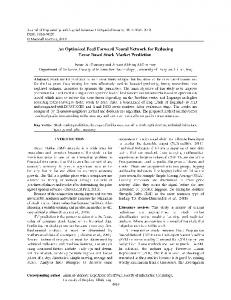
great tool for a simulation study, they are not easy to be implemented neither used. They are dependent on the experience of the user that should answer some questions related to the creation and training process of the neural networks as follows: • What type of artificial neural networks to use? • How many hidden layers, if it a feed-forward is chosen? • How many neurons to be used in input, hidden, and output layers? • What should be the input and the output of the artificial neural network? • How many simulation models are necessary to adequately train an artificial neural network? • What simulation model responses should be selected? • What training algorithm should be used? • Is the trained artificial neural network good enough? Artificial Neural Networks Artificial Neural Networks are “part of a group of analytic tools that attempts to imitate life” (Mohaghegh, 2000). They are algorithms inspired by animals’ brain mechanics that, although they are very simple, can perform a wide variety of tasks like approximate functions, control, pattern recognition, classification, and filtering. The objective of this topic is to present feed-forward neural networks. This is the most common type of artificial neural network used to solve the most challenging problems. Detailed information about artificial neural networks, including other types, can be found in Mohaghegh (2000), Kröse and Smagt (1996), and Demuth et al. (2008). Figure 1 shows the scheme of an artificial neuron. It has the input vector [x1, x2 … xn] which is multiplied by weights [w1, w2 … wn] and a bias represented by “b”. The input and bias are summed and an activation function is used and the result is a output vector Y of dimension 1. Neurons can be grouped in layers like Figure 2 forming a neural network structure called feed-forward. It has this name due to the fact that the information goes through the layers in one way only. There are three types of layers in feed-forward: • Input layer: this layer (blue color) receives the information from outside, i.e. the input parameters of the function that will be approximated (ex. porosity, permeability etc.) It doesn’t have activation function neither bias and has one input per neuron. In this work the number of artificial neurons used is the same of the inputs that will be matched. • Hidden layer: this layer (green color) receives the information from the input layer or from another hidden layer. The activation function can be any, in this work it is used the tan-sigmoid activation function (see Figure 3). The number of hidden layers and of artificial neurons in each hidden layer will to be defined posteriorly. • Output layer: this layer (red color) is the output of the neural network. The activation function can be any, in this work it is used the linear activation function (see Figure 4). The number of neurons is the same of the parameters to be matched in the history matching process (e.g. water production, pressure etc.) The objective of the artificial neural network training is to set the weights and biases so that it can give the same response as the reservoir simulaton model. The elapsed time to obtain a response from neural networks is negligible when compared to reservoir simulation time. This makes the iterative history matching process for a complex reservoir viable. The most common training method used for feed-forward neural networks is back-propagation. In this method, the weights and biases are initially set randomly. A group of pairs of input-output obtained from reservoir simulation models, called training pairs, are selected. The output of training pairs is compared with the output of artificial neural network and the error is calculated by the least squared error in this work. This error represents the “performance function” of the training method. The weights and biases are adjusted from the output layer to input layer iteratively until the performance function becomes small. The success in artificial neural network training depends on the quality of the training pairs. They must represent the multidimensional surface/curve defined by the reservoir simulation as it is an approximation problem. The universal approximation theorem defines that, for a feed-forward neural network and back-propagation training method, “only one layer of hidden units suffices to approximate any function with finitely many discontinuities to arbitrary precision, provided the activation functions of the hidden units are non-linear” (Kröse and Smagt, 1996). This theorem supports the use of a feed-forward neural network with one hidden layer used in this work. Reservoir Simulation Model and History Matching Method The study case of this work is inspired on the model presented by Ertekin et al. (2001), described in some chapters of his book. A heterogeneous model (see Figures 5 and 6) represents the real reservoir which provides the observed data and the homogeneous model represents the initial simulation model. In both models there are three production wells (Well-001, Well003, and Well-005) and two water injection wells (Well-002-I and Well-004-I) and they are initially only oil saturated. Four reservoir parameters (input parameters) were adjusted: porosity, permeability in “x” direction, permeability in “y” direction, and rock compressibility. The least squared error of the water rate production in well Well-005 for the first two years of production was the object function used to validate the quality of the history matching process. The method use was the direct search (Maschio and Schiozer, 2005). The input parameters intervals that will be matched are discretized in this method, so it is easier to find a region with lower object function.

SPE 122148

3

Training the Artificial Neural Network On the light of the previous topics discussions, some decisions were taken. The artificial neural network would be a feedforward with just one hidden layer, four neurons in the input layer (porosity, permeability in “x” direction, permeability in “y” direction, and rock compressibility), one neuron in the output layer (water production rate of well Well-005), and the training method would be the back-propagation (although it was not decided which algorithm yet). The neural network structure defined here cannot describe the whole curve of the water production rate over the time, but just one point of it. So it is necessary to have an extra neuron in the input layer to represent the time in which it was measured the water production rate. A schematic representation of the neural network is presented in Figure 7 with the number of neurons in each layer, except the hidden layer, and the activation function. Similar structures of artificial neural network has been presented in other works like Salehi et al. (2007) and Silva et al. (2006). Selecting the Simulation Models to Be the Training Pairs As presented previously it is important to choose correctly the group of simulation models that will train the artificial neural network. Any property of the reservoir can be defined as a random variable (Jensen et al., 2000). In this way, selecting the values of the properties randomly according to their probability distribution function is the best way to choose the simulation models that will provide the training pairs. If the probability distribution function is not well defined, it is recommended to use the uniform distribution which limits are determined by experts. As artificial neural networks work better if the input and output values are in the interval [-1, 1], it is necessary to parametrize all the properties and answers of the simulation models to this interval before training the neural network. Selecting the Training Algorithm Two training algorithms were compared in this work: gradient descendent algorithm, that is the most simple one, and Levenberg-Marquardt algorithm, that is the one recommended by Demuth et al. (2008). There is a plenty of algorithms available in literature that could be used and programs that provide the scripts already written, what makes the life of the user easier. Another decision that needs to be taken is the number of neurons in the hidden layer. There is not a rule to determine the optimal number of neurons in the hidden layer, but it is recommended to start with the same number of inputs and growing up until the performance function is acceptable (sufficient small). If the number of neurons is too big, the artificial neural network will “memorize” the pairs of training instead of “learning” the surface response of the reservoir simulation. Artificial neural networks with 5, 10, 15 … 50 neurons in the hidden layer were compared, but the selection of the optimal number will be explained in the following paragraphs. A group of 100 simulation models was used to provide the pairs of training. Since the initial values of weights and biases are randomly selected and also that it can heavily interfere in the training result, the training of the artificial neural networks was repeated 100 times, each one having different weights and biases, to provide data for a statistical comparison. The results can be checked in Figures 8 and 9. The Figures show the performance function versus the number of neurons in hidden layer for each training algorithm in three bars: the first is the average of the 100 trainings, the second is the standard deviation and the third is the result of the best training. In Figure 8, the result in the chart is atypical since the best training result and the average should decrease with the number of the neurons. An explanation for this is that we have a convergence problem in the algorithm of gradient descendent once it does not happen with the Levenberg-Marquardt algorithm (see Figure 9). It was decided to use Levenberg-Marquardt algorithm. Choosing the Size of the Training Pair Group In the last item, 100 simulation models were used to decide the training algorithm but it is not necessary the optimal training size. The training pair size is very important and it is defined by the number of simulation models used. If the number of simulation models is small, the artificial neural network will not be able to provide the same response as the simulator. Otherwise, if it is too big, there will have no reason to use the neural network since the solution is close to the original problem, the high number of simulations processed, remains and, maybe, the training algorithm may not converge. Some authors use the “experimental design technique” to select the number of simulation models to be used although it is not proved to work in all cases. In this work, it will be compared groups with 25, 50, and 100 simulation models. Comparing figures 9, 10, and 11, it is possible to observe that the artificial neural networks trained with 25 and 50 simulation models presented similar results, when we compare the average of the 100 trainings and the best training result, and they are better then with 100 simulation models. This last one presents results almost 10 times higher. It can be concluded that the group of 100 simulation models are too big for this study case. The optimal size of the training pair group is a very difficult decision issue in the neural network process. A different group of 200 simulation models were selected to test artificial neural networks with 25 and 50 simulation models. Both artificial neural networks were the best ones with 5 neurons in the hidden layer. The comparison was made using the statistical tool “coefficient of determination” (R2) that shows if a model can explain well the variability in a given variable. In equation (1) (Jensen et al., 2000):

4

SPE 122148

(1)

R2 = 1 −

) ∑( ∑ (Y − Y ) Yi − Yi

2

2

i

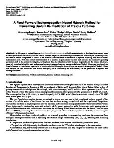
is the predicted value. where Yi is the observed value, Y is the average of the observed values, and Y i With the coefficient of determination, it is possible to compare the artificial neural networks response in an easier way to understand since its value does not have dimension. Values over 0.990 are considered reasonable for general engineering tasks. For this work, values over 0.995 are considered good and values over 0.998 are considered ideal. Figures 12 and 13 provide examples of the coefficient of determination comparing the water rate curves produced by the full reservoir simulator model with the values generated by the artificial neural network model. The coefficient of determination was calculated for the 200 simulation models using the best artificial neural networks trained with 25 and 50 reservoir simulation models. A histogram is presented with the results in Figure 14. It is easy to conclude that the artificial neural network trained with 50 simulation models presents better response than the one trained with 25 simulation models. Selecting the Number of Neurons in Hidden Layers Until this point the following decisions were made: a feed-forward artificial neural network with five neurons in input layer and one in output layer, having only one hidden layer, using Levenberg-Marquardt training algorithm and trained with 50 simulation models. There is still one question to be answered related to the number of neurons in hidden layer. Figure 15 presents a comparison among artificial neural networks with 5, 10, and 15 neurons in hidden layer. Artificial neural network with 10 and 15 neurons presented similar results, but better than 5 neurons. It was decided to use 10 neurons in hidden layer. The History Matching As the artificial neural network is fully defined and trained, it is time to use it in the history matching process. The methodology used in this work is similar to the one presented by Maschio and Schiozer (2005) in which the intervals of the reservoir properties that will be matched are discretized and the history match process searches the point in the multidimensional domain of the reservoir simulator model that has the lowest objective function. The objective function is the least squared error of the water production rate of well Well-005 for the first 2 years of production. A random point, or the initial reservoir model, is selected to start the history match and its objective function is calculated. Then, the objective functions of the points in the neighborhood of the initial point are also calculated. The point in the neighborhood with lowest objective function determines the direction of the search and the property that will be matched in this iteration. The search will continue in this direction/property until the objective function stops decreasing. The last point investigated turns the initial point and the process repeat until the initial point is the minimum in its neighborhood. To avoid being in a local minimum, 10 simulation models were selected randomly to be history matched. Figures 16 and 17 present the result of the history matching for the best simulation model matched. The reservoir simulator responses in the graphs were included only to validate the artificial neural network responses and it can be observed that there is a good correlation between the reservoir simulator and the trained artificial neural network. To perform this history matching without artificial neural networks, it would be necessary over than 900 simulations and, using the methodology proposed in this work, it was used only 50 simulations to train the artificial neural network. The other simulations performed should be disregarded since their objective was to provide statistical data to prove the efficiency of the methodology and would not be necessary in a real application. Moreover, the time spent training the each artificial neural network was too small, approximated 2 minutes in a personal computer with a 1.86 GHz processor speed. Conclusions The methodology proposed in this work was successfully applied in the studied case. The number of simulations necessary to achieve a good history matching results was significantly reduced and this implies directly in a lower processing time and costs without loosing much quality. Some observations should also be presented from the experience of this work: • The use of artificial neural networks is just to approximate functions. Once it was trained, it must be respected the intervals of the properties and they cannot be extrapolated. In this work the artificial neural network was trained for the first two years of water production in well Well-005. This neural network must not be used to forecast the production for the fowling months/years. • A trained artificial neural network must be applied only for the reservoir in study and which it was trained for, if the reservoir model varies drastically, it must be retrained (Taylor made solution). There is not a specific technique to calculate the optimal number of neurons in hidden layer or the number of simulation models to be used in training. The experience of the user must be taken into account. The success in application of the artificial neural network as a reservoir simulation proxy in history matching proves the potential that this tool still has for that petroleum industry.

SPE 122148

5

The studied case presented in this work was very simple and it was easy to train an artificial neural network to work as a proxy for reservoir simulation. The challenges and future work as extension of this work will involve the study of more complexes reservoirs (with faults and more wells, oil, water, and gas saturated, complex behavior etc.), the use of a large number of input properties to be matched, multiple objective functions, and other methodologies of history matching, the application of other types of artificial neural networks (e.g. radial basis networks), and the combination of this tool with other virtual intelligence tools like evolutionary programming and fuzzy logic. References CULLICK, A. S.; JOHNSON, D.; SHI, G. Improved and More-Rapid History Matching With a Nonlinear Proxy and Global Optimization. SPE Annual Technical Conference and Exhibition. San Antonio, Texas: Society of Petroleum Engineers, 2006. DEMUTH, H.; BEALE, M.; HAGAN, M. Neural Network Toolbox™ 6 User’s Guide. The MathWorks, URL:. Date Accessed: December 3, 2008.

2008.

ERTEKIN, T.; ABOU-KASSEM, J. H.; KING, G. R. Basic Applied Reservoir Simulation. 1. ed. Rirchadson, Texas: Society of Petroleum Engineers, 2001. (Textbook, 7). JENSEN, J. L.; LAKE, L. W.; CORBETT, P. W. M.; GOGGIN, D. J. Statistics for Petroleum Engineers and Geoscientists. 2ª. ed. Amsterdam: Elsevier Science, 2000. (Handbook of Petroleum Exploration and Production, 2). KRÖSE, B.; SMAGT, P. V. D. An Introduction to Neural Networks. University URL:. Date Accessed: December 11, 2008.

of

Amsterdam,

1996.

MASCHIO, C.; SCHIOZER, D. J. Comparação entre Metodologia de Otimização Global e o Método de Gradientes para Ajuste de Histórico Assistido. 3º Congresso Brasileiro de P&D em Petróleo e Gás. Salvador, Bahia: Associação Brasileira de Pesquisa e Desenvolvimento em Petróleo e Gás, 2005. MOHAGHEGH, S. Virtual-Intelligence Applications in Petroleum Engineering: Par t 1—Artificial Neural Networks. Journal of Petroleum Technology [S.I.], v. 52, n. 9, p. 8, September 2000. MOHAGHEGH, S. D. Quantifying Uncertainties Associated With Reservoir Simulation Studies Using Surrogate Reservoir Models. 2006 SPE Annual Technical Conference and Exhibition. San Antonio, EUA: Society of Petroleum Engineers, 2006. SALEHI, F.; AZIZI, R.; SALEHI, A. Oil Field Development Using Neural Network Model. Advanced Intelligent Computing Theories and Applications [S.I.], v. 2, p. 10, 2007. SILVA, P. C.; MASCHIO, C.; SCHIOZER, D. J. Evaluation of Neuro-Simulation Techniques as Proxies to Reservoir Simulator. Rio Oil & Gas Expo and Conference 2006. Rio de Janeiro, Brasil: Instituto Brasileiro de Petróleo, Gás e Biocombustíveis, 2006.

Y Figure 1: Scheme of a neuron.

6

SPE 122148

1

1 O

E

O

S

O

S

E

E O Figure 2: Scheme of a feed-forward neural network.

Figure 3: Tan-Sigmoid activation function. (Demuth et al., 2008)

Figure 4: Linear activation function. (Demuth et al., 2008)

Figure 5: Porosity distribution in the heterogeneous reservoir model (Ertekin et al., 2001).

SPE 122148

7

Figure 6: Permeability in “x” direction distribution in the heterogeneous reservoir model in miliDarcy (mD) (Ertekin et al., 2001).

Figure 7: Schematic representation of the neural network. Note: The number of neurons in the hidden layer is a variable to be set yet, so it is represented by the letter n.

Performance Function of the Artificial Neural Networks Varying the Number of Neurons in the Hidden Layer 0,3

Performance Function

0,25 0,2 0,15 0,1 0,05 0 5

10

15

20

25

30

35

40

45

50

Number of Neurons Average of 100 Trainings

Standard Deviation

Best Training Result

Figure 8: Analisys of performance function in artificial neural networks trained with gradient descendent algorithm and 100 simulations.

8

SPE 122148

Perfomance Function of the Artificial Neural Networks Varying the Number the Number of Neurons in the Hidden Layer 0,05


0,045 0,04 0,035 0,03 0,025 0,02 0,015 0,01 0,005 0 5

10

15

20

25

30

35

40

45

50


Standard Deviation


Figure 9: Analisys of performance function in artificial neural networks trained with Levenberg-Marquardt algorithm and 100 simulation models.

Performance Function of the Artificial Neural Network Varying the Number of Neurons in the Hidden Layer 0,006


0,005 0,004 0,003 0,002 0,001 0 5

10

15

20

25

30

35

40

45

50


Standard Deviation



SPE 122148

9

Performance Function of the Artificial Neural Networks Varying the Number of Neurons in the Hidden Layer 0,009


0,008 0,007 0,006 0,005 0,004 0,003 0,002 0,001 0 5

10

15

20

25

30

35

40

45

50


Standard Deviation



Graphic Results of Artificial Neural Network Trained with 50 Simulations Models R2 = 0.9987 500

Water Rate (m3/day)

400 300 200 100 0 0

5

10

15

20

25

30

-100 Time (months) Resevoir Simulator Response

Artificial Neural Network Response

Figure 12: Example of a simulation model with an ideal coefficient of determination. Neural network trained with 50 simulations models.

10

SPE 122148

Graphic Results of Artificial Neural Network Trained with 50 Simulations Models R2 = 0.9954 900 800

Water Rate (m3/day)

700 600 500 400 300 200 100 0 -100

0

5

10

15

20

25

30

Time (months) Resevoir Simulator Response


Figure 13: Example of a simulation model with a good coefficient of determination. Neural network trained with 50 simulation models.

Frequency

Histogram of Coefficient of Determination 140 120 100 80 60 40 20 0 Below 0.990

0.990 and 0.995

0.995 and 0.998

25 Simulation Models

0.998 and 0.999

Over 0.999

50 Simulation Models

Figure 14: Comparison of the best artificial neural networks with 5 neurons in hidden layer trained with 25 and 50 simulation models.

Histogram of Coefficient of Determination 120 Frequency

100 80 60 40 20 0 Below 0.990

0.990 and 0.995

0.995 and 0.998

0.998 and 0.999

5 neurons

10 neurons

15 neurons

Over 0.999

Figure 15: Comparison of the best artificial neural networks with 5, 10, and 15 neurons in hidden layer trained with 50 simulation models.

SPE 122148

11

Comparison of Curves Before History Matching

Water Rate (m3/day)

1000 800 600 400 200 0 -200

0

5

10

15

20

25

30

Time (months) Reservoir Simulator Response Observed Production


Figure 16: Comparison of curves before history matching.

Comparison of Curves After History Matching

Water Rate (m3/day)

800 600 400 200 0 0

5

10

15

20

25

30

-200 Time (months) Reservoir Simulator Response Observed Production


Figure 17: Comparison of curves after history matching.