modelling of the feed forward neural network with its ... - IJAET

International Journal of Advances in Engineering & Technology, Aug., 2015. ©IJAET ISSN: 22311963

MODELLING OF THE FEED FORWARD NEURAL NETWORK WITH ITS APPLICATION IN MEDICAL DIAGNOSIS 1

Stephen Gbenga Fashoto, 2Michael Adeyeye, 3Olumide Owolabi, 4Mba Odim 1

Kampala International University, Kampala, Uganda 2 Sheridan College, Australia 3 University of Abuja Abuja Nigeria 4 Department of Computer Science, Redeemer’s University, Ede, Osun State Nigeria

ABSTRACT This study explores a data mining technique to solve the problem associated with the medical diagnosis of acute inflammations and acute nephritises of the urinary system. Medical diagnosis is a complex classification problem that lacks an analytic or algorithmic solution. The diagnosis problem considered is a classification problem with two types of decision patterns. First, the pattern of the problem is irregular and therefore hard to explicitly derive an analytical or algorithmic solution. Second, the pattern is to determine the classification accuracy reached. Modelling of the data was done using Back Propagation. A feed forward neural network model using six neuron input and varied numbers of hidden neuron was used. The model is trained and tested by partitioning the data into a ratio of four to one (4:1). The four-fifth, which is eighty percent (80%) of the data, is then used for training while the remaining one-fifth, twenty percent (20%), is used for testing the trained neural network model. The output is compared to a known result until the network output error is significantly reduced. The output shows the classification accuracy of the model to be approximately ninety percent (90%), which implies that only one out of ten classifications is incorrect.

KEYWORDS: Medical Diagnosis, Data Mining, Neural Network, Multilayer Perceptron, Back Propagation

I.

INTRODUCTION

Medical diagnostic process is as complicated and complex likes every other diagnostic processes. Patients might not adequately describe how they actually feel and what they are feeling in their body; healthcare providers may perhaps not interpret the information provided by the patients correctly; laboratory results are not immediate and could have some errors. Medical diagnosis, like other diagnostic processes, is made more complex because of the level of imprecision involved. Patients may not be able to describe exactly what has happened to them or how they feel; doctors and other health care practitioners may not understand or interpret exactly what they hear or observe; laboratory reports are not instantaneous and may come with some degree of error (Szolovits, 1988). Medical diagnosis refers to both processes of determining the identity of a possible disease or disorder and opinion reached by the process. Medical diagnosis has always been an art: which brings to mind famous doctors as well as famous painters or composers. An artist, for instance, is someone who is skilled and able carry out imaginative art. This is exactly what a good physician does during a medical diagnosis procedure. A physician employs his education, experiences, and talent, to diagnose a disease. A typical diagnostic procedure usually starts with a patient’s complaints and a doctor learning more about the patient’s situation interactive with him/her during an interview, as well as measure some metrics, such as his/her blood pressure and the body temperature. The diagnosis is then determined by taking the whole available patients’ status into account. Depending on the diagnosis, a suitable treatment is prescribed and the whole process may be iterated. In each of the iterations, the

507

Vol. 8, Issue 4, pp. 507-520

International Journal of Advances in Engineering & Technology, Aug., 2015. ©IJAET ISSN: 22311963 diagnosis might be reconfigured, refined or rejected. Each diagnosis considers diverse symptoms generated by diverse causes which are added to the patient’s background. Epidemics are also considered as well as genetic factors. Only then can a full diagnosis emerge. After a while, the physician would be more experienced, but just gradually and in one branch of medicine. The complexity of the medical diagnosis is revealed in the length of time devoted by medical training compared with other professions. The major task of medical science is to prevent and diagnose diseases. However, this study only focuses on diagnosing diseases, which is not a direct or simple task. Brause (2001) highlighted that almost all physicians are confronted with the task of learning to diagnose during their workmanship. They have to deduce certain diseases and formulate a treatment based on more or less specified observations and knowledge. Listed below are some of the difficulties in medical diagnosis that have to be taken into account: • A sufficient number of experienced cases form the basis for a valid diagnosis and are only achieved in the middle of a physician’s career, not at the end of the programme. This is especially true for rare or new diseases, where the experienced physicians are in the same situation as newcomers. • Particularly, human beings do not resemble statistic or computers but pattern recognition systems. Humans can recognize patterns or objects very easily but will fail, when probabilities have to be assigned to observations. • The quality of diagnosis totally depends on the physician’s talent as well as his/her experiences. • Emotional problems and fatigue degrade the doctor’s performance. • The training procedure of doctors, in particular specialists, is a lengthy and expensive one. So even in developed countries, lack of Medical Directors may be felt. • Medical science is one of the most rapidly growing and changing fields of science. New results disqualify the old treats, and new cures/drugs are introduced day by day. In the same vein, unknown diseases turn up every now and then. So a physician should always try hard to keep him/herself up to date. Regarding problems above and many others, the question would be how computers can help in medical diagnosis. Due to the complexity of the task involved in medical diagnosis, it has not been realistic yet to expect a fully automatic, computer-based, medical diagnosis system. However, recent advances in the field of intelligent systems have facilitated a wider usage of computers, armed with Artificial Intelligence (AI) techniques, in medical diagnosis. Considering the low-cost, high speed and efficiency computers available in the markets today, a good number of patients can be attended to with a well designed intelligent diagnostic system. This will provide physicians the opportunity to focus on more serious cases. Hence, this paper attempts to provide a relatively efficient solution for designing a prompt medical diagnosis using the Data Mining technique called Neural Networks. Although AI has severally been employed in medical diagnosis, effective diagnostics systems are still desirable (Djam & Wajiga, 2012). Physicians have not fully accepted conventional decision support systems for the following reasons: a) Medical field is so complex and complicated that Safety is paramount. To this effect, physicians are concerned about the accuracy of decision support systems (Kim et al 2008). b) Most Decision support system is design is such a way that is not very easy for user to make use of it or have a good understanding of what the system is all about, which is the causes of the indifference in the utilization of the DSS (Khan et al 2000) . c) The physicians believe in their absolute knowledge of medical phenomena, and become averse to consultative suggestions by computer-based decision support systems (Berner, & Graber, 2008). The foregoing clearly suggests that medical diagnosis is a complex classification problem that analytically lacks algorithmic solution. Therefore we have explored a data driven approach and a data mining technique to solve the problem. Data Mining is concerned with the design and development of mechanisms that allow computers to evolve behaviour based on knowledge gained from the dynamic observation process. To this end, we explored a multilayer neural network with the back-propagation algorithm that can learn from examples, capture and classify subtle functional relationships among the data even when the underlying relationships are unknown or hard to describe. The remaining part of this paper is organized as follows. Section 2 describes literature review. Section

508

Vol. 8, Issue 4, pp. 507-520

International Journal of Advances in Engineering & Technology, Aug., 2015. ©IJAET ISSN: 22311963 3 presents the methodology. Section 4 describes the implementation and Section 5 concludes the paper.

II.

LITERATURE REVIEW

In Neural Network domain solution to problems can be achieved without knowledge of the problems. Neural network can solve problems in as much as there is a known number of attributes to a particular problem with predicted result. This is a very helpful tool for discovering hidden information. However, expert systems have been developed by researchers to diagnose and solve complex medical problems such as the diagnosis of acute inflammation and acute nephritis in urinary system. Supervised learning methods such as support vector machine (SVM), K-nearest neighborhood (KNN) have also been used for medical diagnosis. The initial attempt at creating a decision making tools started by applying statistical techniques to medical diagnosis pioneered by Lipkin, Hardy, and Engle in the 1950s (Kulikowski, 1987). This later paved way for Artificial intelligence (AI) due to the inadequacy of the statistical techniques to solve complex medical problems (Gorry, 1973). Heckerling et al (2007) used artificial neural networks (ANN) coupled with genetic algorithms to evolve combinations of clinical variables optimized for predicting urinary tract infection. Mazurowski et al (2008) investigated the effect of class imbalance in training data when developing neural network classifiers for computer aided medical diagnosis. The investigation is performed in the presence of other characteristics that are typical among medical data, namely small training sample size, large number of features, and correlations between features. Zhang et al (2008) presented a method for developing a fully automated Computer aided diagnosis system to help radiologist in detecting and diagnosing micro-calcifications in digital format mammograms. Higuchi, et al (2006) tested a three-layered artificial neural network analysis of phonocardiogram recordings to diagnose, automatically and objectively, the condition of the heart in patients with heart murmurs. Medical Diagnosis using Artificial Neural Networks is currently a very active research area in medicine and it is believed that it will be more widely used in biomedical systems in the next few years. This is primarily because the solution is not restricted to linear form. Neural Networks are ideal in recognizing diseases using scans since there is no need to provide a specific algorithm on how to identify the disease. Neural networks learn by example so the details of how to recognize the disease is not needed.

2.1 Data Mining Data Mining (DM) is an aspect of Computer Science that is very recent and employ statistical techniques such as artificial intelligence, database and so on. The basis of the methodologies of DM can be found in the integration of statistical methods into artificial intelligent techniques for administering databases and its capability to discover patterns and correlations contained by large amount of data that will enable the creation of models (Malucelli et al., 2010; Worachartcheewan et al., 2010). 2.1.1 Descriptive and Prescriptive Data Mining 2.1.1.1 Descriptive Data Mining The descriptive DM identifies the patterns or relationships in data and explores the properties of the data examined (Deshpande & Thakare, 2010). It describes all the data, it includes models for overall probability distribution of the data, partitioning of the p-dimensional space into groups and models describing the relationships between the variables. Clustering, association rule discovery, sequence discovery and summarization are some of the examples of descriptive data mining. 2.1.1.2 Prescriptive Data Mining Modelling Predictive modeling permits the value of one variable to be predicted from the known values of other variables. Classification, Regression, Time series analysis, Neural Networks etc are some examples of prescriptive data mining modeling. Tan et al. (2009) pointed out that several DM applications aimed to predict imminent state of the data. Prediction is the ability to analyze the past and current attributes to determine the future state.

509

Vol. 8, Issue 4, pp. 507-520

International Journal of Advances in Engineering & Technology, Aug., 2015. ©IJAET ISSN: 22311963 2.2 Neural Networks An Artificial Neural Network (ANN), often just called a "Neural Network" (NN), is a mathematical model or computational model, in other words, they imitate the way the human brain learns and use rules inferred from data patterns to construct hidden layers of logic for analysis (Singh & Chauhan, 2005). NNs constitute the most widely used technique in DM. According to Hajek (2005) a NN is a massively parallel-distributed processor that has a natural tendency for storing experiential knowledge and making it available for use. It resembles the brain in two respects: (i) Knowledge is acquired by the network through a learning process; and (ii) Interneuron connection strengths known as synaptic weights are used to store the knowledge. A NN is a graph, with patterns represented in terms of numerical values attached to the nodes of the graph and transformations between patterns achieved via simple message-passing algorithms (Jordan & Bishop, 1996). NN topologies can be divided into feed-forward and recurrent classes according to their connectivity (Yao, 1999; Singh & Chauhan, 2005). The feed-forward neural network was the first and arguably simplest type of artificial neural network devised. In this network, the information moves in only one direction, forward, from the input nodes, through the hidden nodes and to the output nodes. A NN is feed forward if there exists a method, which numbers all the nodes in the network such that there is no connection from a node with a large number to a node with a smaller number. All the connections are from nodes with small numbers to nodes with larger numbers. A NN is recurrent if such a numbering method does not exist. Contrary to feed-forward networks, Recurrent Neural Networks (RNs) are models with bidirectional data flow. While a feed forward network propagates data linearly from input to output, RNs also propagate data from later processing stages to earlier stages. Learning in ANN can roughly be divided into supervised, unsupervised, and reinforcement learning (Yao, 1999; Singh & Chauhan, 2005). Supervised learning or associative learning is based on direct comparison between the actual output of an ANN and the desired correct output, also known as the target output. The reinforcement learning is a special case of supervised learning where the exact desired output is unknown. It is based only on the information of whether or not the actual output is correct. The unsupervised learning is solely based on the correlations among input data. No information on “correct output” is available for learning. According to Larose (2006) there are two general categories of neural net algorithms: supervised and unsupervised. Supervised neural net algorithms such as Back propagation and Perceptron require predefined output values to develop a classification model. Among the many algorithms, Back propagation is the most popular supervised neural net algorithm (Han & Kamber, 2006). Unsupervised neural net algorithms do not require predefined output values for input data in the training set and employ self organizing learning schemes to segment the target dataset. For organizations with a great depth of statistical information, ANNs are ideal because they can identify and analyze changes in patterns, situations, or tactics far more quickly than any human mind, as indicated by Guo (2003). Although the neural net technique has strong representational power, interpreting the information encapsulated in the weighted links can be very difficult. One important characteristic of neural networks is that they are opaque, which means there is not much explanation of how the result was obtained and what rules are used. There are two types of Neural Networks based on network topology and these are: (i) Feed-Forward Neural Network (FFNN) and (ii) Feed-Back Neural Network (FBNN). i) Feed-Forward Neural Networks In Feed-Forward Neural Networks (FFNNs), information moves only in the forward direction from the input layers, via the hidden layers (if any) and to the output layers. The FFNNs were the first and most widely used models in many practical situations. They can match the input vectors and the output vectors. The output at any particular time is dependent on only the corresponding input. This is because FFNNs are easily to train and they produce a response to an input quickly. Examples of feed-forward networks include the single-layer perceptron, ADALINE, multilayer perceptron, radial basis function, learning vector quantization network, probabilistic neural network, generalized regression neural network, etc. ii) Feed-Back Neural Networks

510

Vol. 8, Issue 4, pp. 507-520

International Journal of Advances in Engineering & Technology, Aug., 2015. ©IJAET ISSN: 22311963 In the Feed-Back Neural Networks (FBNNs), there are feedback connections from one layer to another. That is, there is a bi-directional data flow and data are also propagated from the outputs to the input layers. These types of networks have a dynamic memory in that any particular output is a function of the current input and past inputs and outputs. FBNNs are best suited for optimization problems where the neural network looks for the best arrangement of interconnected factors. They are also used for error-correction and partial-contents memories where the stored patterns correspond to the local minima of the energy function. Examples of feed-back neural networks include Boltzman machine, Elman networks, recurrent network, and so on. 2.2.1 Multilayer Perceptron A Multilayer Perceptron is a feed-forward artificial neural network that maps sets of input data onto a set of appropriate output. It is a modification of the standard linear perceptron in that it uses three or more layers of neurons (nodes) with nonlinear activation functions, and is more powerful than the single perceptron in that it can distinguish data that is not linearly separable, or separable by a hyperplane (Chandra et al., 2007).The error signals are used to calculate the weight updates which represent knowledge learnt in the networks. The performance of back propagation algorithm can be improved by adding a momentum term (Quinlan, 1993; Setiono & liu, 1995).The error in back propagation algorithm is minimized by using equation 1 formula. (1) 2.1 ) Where n=number of epochs, ti is desired target value associated with ith epoch and yi is output of the network. To train the network with minimum possibility of error we adjust the weights of the network (Setiono & Liu, 1995; Rudy & Huan, 1995).

III.

METHODOLOGY

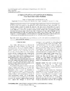
We employ multilayer artificial neural networks for the study with back propagation algorithm. Multilayer neural networks emerged to overcome the practical limitations of the perceptron and the LMS (Least Mean Square) algorithms (Haykin, 2009). The basic features of the multilayer perceptron include: • A model of each neuron in the network, which includes a nonlinear activation function that is differentiable. A network containing one or more layers that are hidden from both input and output nodes. • A network that exhibits a high degree of connectivity, the extent of which is determined by synaptic weights of the network.

Figure 1: A multilayer feed forward network using a supervised learning algorithm.

Among the supervised learning algorithms is the back propagation shown in Figure 1.

3.1 Back Propagation Minsky & Papert (1969) showed that there are many simple problems such as the exclusive-or problem, which linear neural networks cannot solve. The term "solve" means to learn the desired associative links. The argument is that if such networks cannot solve such simple problems, then it

511

Vol. 8, Issue 4, pp. 507-520

International Journal of Advances in Engineering & Technology, Aug., 2015. ©IJAET ISSN: 22311963 would be impossible to solve complex problems in computer vision, natural language processing, and motor control. Solutions to this problem were as follows: a) Select appropriate "recoding" scheme which transforms inputs b) Perceptron Learning Rule -- Requires that one correctly "guesses" an acceptable input to hidden unit mapping. c) Back-propagation learning rule -- Learn both sets of weights simultaneously. Back propagation is a form of supervised learning for multilayer networks. Error data in the output layer is "back propagated" to earlier ones, allowing incoming weights to these layers to be updated. It is most often used as a training algorithm in the current neural network applications. The back propagation algorithm was developed by Paul Werbos in 1974 and rediscovered independently by Rumelhart et al.(1986). Since its rediscovery, the back propagation algorithm has been widely used as a learning algorithm in feed forward multilayer neural networks. The algorithm is different from the other algorithms in the process given that weights are calculated during the learning process. In general, the difficulty with Multilayer Perceptron is calculating the weights of the hidden layers in an efficient way that can result in the least (or zero) output error. The more hidden layers there are, the more difficult it becomes to calculate the weights. To update the weights, one must calculate an error. At an output layer this error is easily measured; this is the difference between the actual and desired (target) outputs. At the hidden layers, however, there is no direct observation of the error. Hence, some other technique must be used to calculate the error at the hidden layers that will cause minimization of the output error, as this is the ultimate goal. The back propagation algorithm is a good mathematical tool and the execution of the training equations is based on iterative processes. As a result, it is easily implemented on a computer. According to Kwon (2014), an important consideration of the back propagation algorithm is its complexity, that is, the amount of time or resources that it requires to solve a problem. 3.1.1 Types of Back Propagation Training According to Paulin & Santhakumaran (2011), there are many variations of the back propagation algorithms, four of which are described as follows: i) Steepest Descent Algorithm This is a first-order algorithm utilizing first-order derivative of total error function. The result is used to determine the minima error space. The algorithm is denoted by gradient g which is represented by equation (2): g=

=

(2)

With the definition of gradient g in (equation 3), the update rule of the steepest descent algorithm could be written as (3) Where

is the learning constant (step size). The training process of the steepest descent algorithm is asymptotic convergence. Around the solution, all the elements of gradient vector would be very small and there would be a very tiny weight change. ii) Newton’s Method Newton’s method assumes that all the gradient components g1, g2, …, gN are functions of weights and all weights are linearly independent: gi = Fi (wi) (4) where i = 1, 2, …, N Where F1, F2,… FN are nonlinear relationships between weights and related gradient components. Unfold each g1 (i = 1, 2,…, N) in Equations 4 by Taylor series and take the first-order approximation: gi = gi0 +

(5)

where i=1,2,……, N By combining the definition of gradient vector g in (3), it could be determined that

512

Vol. 8, Issue 4, pp. 507-520

International Journal of Advances in Engineering & Technology, Aug., 2015. ©IJAET ISSN: 22311963 (6) By inserting Equation 6 to 5 gives equation 7: gi = gi0 +

(7)

where i=1,2,……, N Comparing with the steepest descent method, the second-order derivatives of the total error function need to be calculated for each component of gradient vector. In order to get the minima of total error function E, each element of the gradient vector should be zero. Therefore, left sides of the Equations 7 are all zero, then 0≈ gi0 +

(8)

where i = 1, 2, … N By combining Equation 3 with 8

- gi0 ≈ Where i=1,2, …., N There are N equations for N parameters so that all weight space can be updated iteratively. Equations 9 can be also written in matrix form

=

(9) can be calculated. With the solutions, the

=

where the square matrix is Hessian matrix:

(10) By combining Equations 3 and 10 with Equation 9 (11) So (12) Therefore, the update rule for Newton’s method is (13) As the second-order derivatives of total error function, Hessian matrix H gives the proper evaluation on the change of gradient vector. iii) Gauss – Newton Algorithm

513

Vol. 8, Issue 4, pp. 507-520

International Journal of Advances in Engineering & Technology, Aug., 2015. ©IJAET ISSN: 22311963 If Newton’s method is applied for weight updating, in order to get Hessian matrix H, the second-order derivatives of total error function have to be calculated and it could be very complicated. In order to simplify the calculating process. Jacobian matrix J is introduced as

(14) Obviously, the advantage of the Gauss-Newton algorithm over the standard Newton’s method is that the former does not require the calculation of second-order derivatives of the total error function, by introducing Jacobian matrix J instead. However, the Gauss-Newton algorithm still faces the same convergent problem like the Newton algorithm for complex error space optimization. Mathematically, the problem can be interpreted as the matrix JTJ may not be invertible. iv) Levenberg-Marquardt Algorithm The Levenberg-Marquardt(LM) algorithm (Levenberg, 1944; Marquardt, 1963), which was independently developed by Kenneth Levenberg and Donald Marquardt, provides a numerical solution to the problem of minimising a non-linear function. As the combination of the steepest descent algorithm and the Gauss-Newton algorithm, the Levenberg-Marquardt algorithm switches between the two algorithms during the training process. The LM is utilized in this study because it combines the features of steepest descent and Gauss Newton algorithm and it is also fast with a stable convergence. Secondly, in the artificial neuralnetworks field, this LM algorithm is suitable for training small and medium sized problem.

3.2 Data Collection In this study, 120 datasets are collected from University of California Irvine (UCI) repository and these served as the knowledge source for this study. The data is separated into inputs and targets. The attributes selected will act as the inputs to the Multilayer Perceptron using Back Propagation algorithm. The targets for the feed-forward neural network will be identified with 1's as decision1 (Acute Inflammation) and 0's as decision2 (Acute Nephritis). They defined the relevant attributes in taken decisions for diagnosing urinary diseases such as the acute inflammation and acute nephritis. Acute inflammation will occur when a patient feels any pains in the abdomen area and there is constant urine coming out (urine_pushing) due to micturition pains and deficiency of urine keeping at maximum temperature of 38oC. Acute nephritis will occur when there is a symptom of fever at a minimum temperature of 40oC and it is commonly found in women than in men. The sign of a fever comes with a patient shaking with lumbar pains on one side or both sides which will be very strong. The dataset containing the attributes indicated in Table 1 is fed into the Neural Network toolbox of MATLAB 2013 to generate the percentage of the classification of decision of diseases of the patient being diagnosed. A feed forward neural network model using six neuron input and varied numbers of hidden neuron is used. The model is trained and tested by partitioning the data into a ratio of four to one (4:1). The four-fifth, which is eighty percent (80%) of the data, is then used for training while the remaining one-fifth, twenty percent (20%), is used for testing the trained neural network model. The attributes (Temperature, Nausea, Lumbar_pain, Urine_pushing, Micturition_pains and Urethra_pains) and the decisions(decision1 and decision2) are used to determine the classification accuracy of the model. The Table 1 shows the list of attributes and decisions used in this study.

514

Vol. 8, Issue 4, pp. 507-520

International Journal of Advances in Engineering & Technology, Aug., 2015. ©IJAET ISSN: 22311963 Table 1: Attribute Selection on Urinary medical Details Attributes Name Temperature Nausea Lumbar_pain urine_pushing micturition_pains urethra_pains Decision1(Acute Inflammation) Decision2(Acute Nephritis)

Data type Numeric Nominal Nominal Nominal Nominal Nominal Nominal Nominal

3.3 Normalization The normalization process for the raw inputs has great effect on preparing the data to be suitable for the training. Without this normalization, training would have been very slow. There are many types of data normalization. It can be used to scale the data in the same range of values for each input feature in order to minimize bias. Data Normalization standardize the raw data by converting them into specific range using linear transformation which can generate good quality clusters and improve the accuracy of clustering algorithms. Data normalization can also speed up training time by starting the training process for each feature. Neural network could achieve a better performance by processing the network input and target before presenting them for network use. The processing of the input data is done with normalization procedure before subjecting the data to network use. The processing is to eliminate any discrepancy with mixed variable of large and small magnitude which may be difficult for learning algorithm for figure out the importance level and may subsequently reject variable with less magnitude (Tymvios et al., 2008). This is one of the major benefits of normalization procedure on training data as well as increased speed of training in the neural network. The normalization procedure can also help to handle input with varied scale which is useful to applications that have input on a widely different scale. There are many types of data normalization and they implement techniques such as product rule, sum rule, min rule, max rule and so on. i) Z-Score Normalization The technique applies mean and standard deviation across training data set to normalize the features of each input vector. The computation of the mean and standard deviation of each feature is then performed. The equation to achieve the transformation is given as (3.1) The output result with a zero mean and unit variance for each of the features. In order to achieve the output, normalization on all the feature vectors is performed. This result in a new training set on which mean and standard deviation are computed. However, the training set need be retained to serve as weight in the final design. The process enumerated above is called pre-processing stage of the neural network structure which significantly improves the performance of the overall network as opposed to using un-normalized data. It also eliminates the effects of outliers in the data. ii) Min-Max Normalization The technique used for normalization is performed using linear transformation on the raw data. X Min and XMax represent the minimum and maximum values for the attribute X which is mapped between the range of 0 and 1. The technique used in computation of Min-Max normalization is shown by equation (3.2) (15) The min-max normalization can also be scaled into range of [-1, 1] using the equation (3.3) below (16) iii) Median Normalization

515

Vol. 8, Issue 4, pp. 507-520

International Journal of Advances in Engineering & Technology, Aug., 2015. ©IJAET ISSN: 22311963 The median method normalizes each sample by the median of raw inputs for all the inputs in the sample. It is a useful normalization to use when there is a need to compute the ratio between two hybridized samples. Median is not influenced by the magnitude of extreme deviations. It can be more useful when performing the distribution. (17) iv) Sigmoid Normalization The sigmoid normalization function is used to scale the samples in the range of 0 and is used to scale the samples in the range of 0 and 1 or -1 to +1. There are several types of non-linear sigmoid functions available. Out of that, tan sigmoid function is a good choice to speed up the normalization process. If the parameters to be estimated from noisy data the sigmoid normalization, method is used. (18) v) Mean and Standard Deviation Normalization This technique scales the network inputs and targets by concentrating on the mean and standard deviation of the training set. The network inputs and targets are normalized to obtain zero mean and a unit standard deviation. A system that applies this technique in pre-process stage for training data set must use a new set of input for the trained network. The new data set can then the trained along with the mean and standard deviation of the previously pre-process data of the original data set. The computation is achieved using: (

–

x

+

(19)

(Jayalakshmi & Santhakumaran, 2011) In this study we employed the sigmoid Normalization method, first to remove biases from the dataset and second, because the values of most of the attributes are in the interval of 0 and 1. Mago et al. (2012) found that the sigmoid function is more suitable for medical diagnosis that was the third reason why the sigmoid normalization method was adopted for this study.

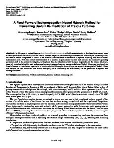
3.4 Experimental Setup In this paper, we use a 3 hidden layer network for our design. The training for the network involves the following steps: Start Initialize the weights in the network (often randomly) Do For each example e in the training set O = neural-net-output(network, e) ; forward pass T = teacher output for e Calculate error (T - O) at the output units Compute delta_wh for all weights from hidden layer to output layer; backward pass Compute delta_wi for all weights from input layer to hidden layer; backward pass continued Update the weights in the network Until all examples classified correctly or stopping criterion satisfied Return the network End The network consists of six input variable, denoting the symptoms of the diagnosis, two output neurons, each for a particular diagnosis category. We vary the number of neurons of the hidden layer and compared with the output the network output error was totally reduced. Figure 2 depicts the model.

516

Vol. 8, Issue 4, pp. 507-520

International Journal of Advances in Engineering & Technology, Aug., 2015. ©IJAET ISSN: 22311963 Output Layer

Hidden Layer

Input Layer

Nausea

Decision

1

Lumbar Pain

Urine Pushing

Micturition Pains

Decision 2

Urethra Pains Micturitio n

Figure 2: The Multilayer Network for our model

IV.

IMPLEMENTATION

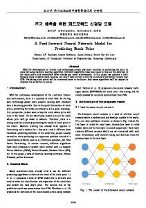
This section describes the implementation of the Back propagation algorithm in building the neural networks to diagnose the two diseases of the urinary system as discussed earlier. The graph on figure 3 of the training session showed the training functions tested with the network. It was observed that Levenberg Marquardt(trainlm) give optimum performance at 78 epochs. Samples of the trained data were taken and used to train the network using various epochs until the network outputs were very close to known results, which means that the error has been totally reduced. The testing result showed that the model accuracy for classification was 90%. This means that out of every 10 classifications made only one is incorrect. Performance is 9.95904e-006, Goal is 1e-005

0

10

-1

Training-Blue Goal-Black

10

-2

10

-3

10

-4

10

-5

10

-6

10

0

10

20

30

40 78 Epochs

50

60

70

Figure 3: Learning Curve

V.

CONCLUSION

There is a growing trend in the use of neural network solution in the medical domain. With increased level of acceptance of medical diagnosis technology which is viable tool that can assist physicians and other health professionals in decision making. Having implemented and tested the Neural Network (NN) solution based on the use of back propagation algorithm for training, we have discovered that

517

Vol. 8, Issue 4, pp. 507-520

International Journal of Advances in Engineering & Technology, Aug., 2015. ©IJAET ISSN: 22311963 with NN, it is possible to implement the human intelligence for medical diagnosis. With traditional techniques, one must understand the inputs, the algorithms, and the outputs in great detail before one can implement a solution. With ANN, one simply shows it: "this is the correct output, given this input". With an adequate amount of training, the network will mimic the function being demonstrated. Using the Back propagation algorithm with early stopping generalization method to build network can effectively avoid the problem of over fitting in neural network models. The output shows the classification accuracy of the model to be approximately ninety percent (90%), which implies that only one out of ten classifications is incorrect.

REFERENCES [1]. Berner, E., & Graber, M. (2008). Overconfidence as a cause of diagnostic error in medicine. The American journal of medicine, 121(5), pp. 2-23 [2]. Chandra, D., Ravi, V., & Ravisankar, P. (2007). Support Vector Machine and Wavelet Neural Network hybrid: Application to Bankruptcy Prediction in Banks. International Journal of Data Mining, Modeling and Management 1(2): pp. 1-21. [3]. Deshpande, S., & Thakare, V. (2010). Data Mining System and Applications: A Review. International Journal of Distributed and Parallel Systems (IJDPS), 1(1), pp. 32-44. [4]. Djam, X., & Wajiga, G. (2012). A Novel Diagnostic Framework: The Application of Soft Computing Technology. The Pacific Journal of Science and Technology, 13(1). [5]. Djam, X., Wajiga, G., Kimbi, Y., & Blamah, N. (2011). A Fuzzy Expert System for the management of Malaria. Int. J. Pure Appl. Sci. Technol., 5(2) , pp. 84-108. [6]. Duch, W., Adamczak, R. & Grąbczewski, K. (2001). A New Methodology of Extraction, Optimization and Application of Crisp and on Neural Networks 12, pp. 277-307 Fuzzy Logical Rules., IEEE Transactions . [7]. Duch,W., Setiono, R., & Żurada, J. (2004). Computational Intelligence Me Rule-Based Data Understanding. Proceedings of the IEEE, Volume:92 , Issue: 5. [8]. Guo, L. (2003). Applying Data Mining Techniques in Property and Casualty Insurance. USA. http://www.casact.org/pubs/forum/03wforum/03wf001.pdf Access date: December 4, 2010. [9]. Hajek, M. (2005). Neural Networks. http://www.cs.ukzn.ac.za/notes/neuralnetworks2005.pdf access date: December 25, 2010. [10]. Han, J., & Kamber, M. (2006). Data Mining: Concepts and Techniques, 2nd edition, Morgan kufman Publishers, San Francisco. [11]. Haykin, S. (2009). Neural Networks and Learning Machine (3rded.). Pearson Education , New Jersey. [12]. Heckerling, P.,Canaris,G., Flach,S., Tape,T.,Wigton,R., & Gerber,B. (2007). Predictors of urinary [13]. tract infection based on artificial neural networks and genetic algorithms. International [14]. Journal of Medical Informatics;Vol.76, No.4, pp. 289-296. [15]. Higuchi, K., Sato, K., Makuuchi, H., Furuse, A., Takamoto, S. & Takeda, H. (2006). Automated diagnosis of heart disease in patients with heart murmurs: application of a neural network technique. Journal of Medical Engineering & Technology, Vol.30, No.2, pp. 61-68. [16]. Jayalakshmi, T., & Santhakuruman, A. (2011). Statistical Normalization and Back Propagation for [17]. Classification. International Journal of Computer Theory and Engineering, 3(1), pp. 89-92. [18]. Jordan, M., & Bishop, C. (1996). Neural Networks. ACM Computing Surveys 28(1), pp. 73–75. [19]. Khan, M., Chong, A., & Quaddus, M. (2000). Fuzzy cognitive maps and intelligent decision support– A review. School of Information Technology, Murdoch University, Graduate School of Business. [20]. Kim, M., Kim, C., Hong, S., & Kwon, I. (2008). Forward–backward analysis of RFID- enabled supply chain using fuzzy cognitive map and genetic algorithm. Expert Systems with Applications, 35(3), pp. 1166-1176 [21]. Larose, T. (2006). Data Mining Methods and Models, John Wiley & Sons Inc. Publisher,Hoboken: New Jersey. [22]. Levenberg, K. (1944). A Method for the Solution of Certain Non-Linear Problems in Least Squares. The Quarterly of Applied Mathematics, 2: pp. 164-168. [23]. Mago, V., Mehta, R., Woolrych, R., & Papageorgiou, E. (2012). Supporting meningitis diagnosis amongst infants and children through the use of fuzzy cognitive mapping. BMC medical informatics and decision making, 12(1), pp. 98. [24]. Malucelli, A., Stein-Junior, A., Bastos, L., Carvalho, D., Cubas, M., & Paraiso, E. (2010). Classification of risk Micro-areas using data mining. Rev Saude Publica. 44(2), pp. 292-300. [25]. Marquardt , D. (1963).An algorithm for least square estimation of nonlinear parameters. SIAM Journal Appl. Math., 11, pp. 431-441.

518

Vol. 8, Issue 4, pp. 507-520

International Journal of Advances in Engineering & Technology, Aug., 2015. ©IJAET ISSN: 22311963 [26]. Mazurowski, M., Habas, P., Zurada, J., Lo, J., Baker, J. & Tourassi, G. (2008). Training Neural Network Classifiers for Medical Decision Making: The Effects of Imbalanced Datasets on Classification Performance. Special Issue on Advances in Neural Networks Research:IJCNN ’07, 2007 International Joint Conference on Neural Networks IJCNN’07 Orlando, Florida, USA, April, 2008, Vol.21, No.3, pp. 427-436, Available at http://ci.louisville.edu/zurada/publications/mazurowski.nn.2008.pdf. [27]. Minsky, M., & Papert, S. (1969). Perceptrons. Cambridge, MA: MIT Press. [28]. Paulin, F., & Santhakumaran, A. (2011). Classification of breast cancer by comparing back propagation training algorithms. Int. J. Comput. Sci. Eng., 3: pp. 327-332. [29]. Quinlan, J. (1993). C4.5: Programs for Machine Learning. Morgan Kaufmann. [30]. Rudy, S., & Huan, L. (1995). NeuroLinear: From neural networks to oblique decision rules. Neurocomputing Journal. [31]. Rumelhart, D., Hinton, G., & Williams, R. (1986). Learning internal representations by error propagation. In E. and Rumelhart, D. McClelland, J. L., editors, Parallel Distributed Processing: Explorations in the Microstructures of Cognition, volume 1,pp. 318_362. MIT Press, Cambrigde, MA. [32]. Rumelhart, D., Hinton, G., & Williams, R. (1986). Learning Internal Representations by Error Propagation. Parallel Distributed Processing, MIT Press, 918-362. [33]. Setiono, R., & Liu, H. (1995). Understanding neural networks via rule extraction, the 14th Int. Joint Conf. on Artificial Intelligence, pp. 480-485, Montreal, Canada. [34]. Siddharth, J., & Shruthi,K.(n.d ) A Two Tier Neural Inter-Network Based Approach to Medical Diagnosis Using K-Nearest Neighbor Classification for Diagnosis Pruning, Available at http://infolab.stanford.edu/~jonsid/nimd.pdf. [35]. Singh, Y., & Chauhan, S. (2005). Neural Networks in Data Mining’, Journal of Theoretical and Applied Information Technology, pp. 37-42. [36]. Sordo, M. (2002). Introduction to Neural Networks in Healthcare. OpenClinical, Available at http://www.openclinical.org/docs/int/neuralnetworks011.pdf. [37]. Szolovits, P., Patil, R., & Schwartz W. (1988). Artificial Intelligence in Medical Diagnosis. Annals of Internal Medicine, 108(1):80-87. [38]. Tan, P., Steinbach, M. & Kumar, V. (2009). Introduction to Data Mining, 3rd edition, Pearson Education, New Delhi. [39]. Tymvios, F., Costantinides, P., Retalis, S., Paronis, S., Evripidou, P., & Kleanthous, S. (2008). The AERAS project: data base implementation and Neural Network classification tests. Urban Air Quality Proceedings. [40]. Werbos, P. (1974). Beyond regression: new tools for prediction and analysis in the behavioral science. Doctoral Dissertation, Harward, Cambridge, MA, U.S.A. [41]. Worachartcheewan, A., Nantasenamat C., Isarankura-Na-Ayudhya C., Pidetcha, P. & Prachayasittikul, V. (2010): Identification of metabolic syndrome using decision tree analysis. Diabetes Res Clin Pract , 90(1):pp. 15-18. [42]. Yao, X. (1999). Evolving Artificial Neural Networks. Proceedings of the IEEE, Vol. 87(9), pp. 14231447. [43]. Zhang, G., Yan,P., Zhao, H. & Zhang, X.(2008). A Computer Aided Diagnosis System in Mammography Using Artificial Neural Networks. International Conference on BioMedical [44]. Engineering and Informatics, Vol.2, pp. 823-826.

AUTHOR BIOGRAPHIES Stephen Gbenga Fashoto is presently a Senior Lecturer in Department of Computer Science in a University in Kampala, Uganda. He obtained his B.Sc. (Honours) in Computer Science and Mathematics, M.Sc in Computer Science and Ph.D in Computer Science. He has several publications in journals (local and international) and Conference proceedings (both local and international). He is a member of Computer Professionals of Nigeria(CPN) and IAENG. He has over ten years of teaching experience in the University. His research interests are in health informatics, Bioinformatics, Application of Data Mining techniques, Application of Cryptography algorithms and Application of optimization techniques such as AHP and TOPSIS.

519

Vol. 8, Issue 4, pp. 507-520

International Journal of Advances in Engineering & Technology, Aug., 2015. ©IJAET ISSN: 22311963 Michael Adeyeye works with a University in Australia. He is also a technical consultant at the Mozilla Co-orporation, USA. Before now, he was a (senior) lecturer and researcher at two of the South African universities (University of Cape Town and Cape Peninsula University of Technology). And before taking roles in South Africa, he worked for the Covenant University, Nigeria and the Embassy of the Untied States, Nigeria. As a Mozillian, he hacks the Mozilla codebase to create innovative solutions. He developed the Transfer HTTP Firefox extension, which led to WebRTC - a browser-to-browser mechanism that is now being standardized by the Internet Engineering Task Force (IETF) and the World Wide Web Consortium (W3C). He currently finds and fixes bugs for FirefoxOS as well as integrates new features in the firmware. He is a sustaining member of the Internet Society and a member of the IEEE. He has attended a number of standardization meetings like the IETF. He earned his second Master and Ph.D. degrees at the University of Cape Town. His research interests include Wireless Mesh Networks, Web and multimedia service mobility technologies, context awareness, multimodal and multi-channel access, information systems, and Next Generation Network (NGN) applications and services. As a researcher, he has extensively published in a number of flagship conference proceedings and journals. He has also immensely contributed to a number of open source projects and initiatives. He is a thinker, hacker and explorer of disruptive technologies. He with his team members has pioneered a number of projects in the global space, such as the first to prototype a browserto-browser communication mechanism, the first to start a wireless mesh network group in West Africa, the first to demonstrate how to use cryto-currencies (bitcoin) for intra-Africa trade, the first to develop few Internet of Things solutions to address topical problems in Africa, e.t.c. Lastly, he is a technical, academic and community specialist, who has widely travelled across the globe working for corporations, governmental and nongovernmental/non-profit organizations. Olumide Owolabi obtained a Ph.D. in Computer Science from the University of Strathclyde, Glasgow. He has taught at the University of Port Harcourt and the University of Abuja, all in Nigeria. He has published extensively in the areas of databases, intelligent information systems and data mining. He is currently the ICT Director at University of Abuja. He is a member of the Nigeria Computer Society(NCS), Computer Professionals Registration Council of Nigeria(CPN) and the Open Source Foundation of Africa (FOSSFA).

Mba Obasi Odim obtained B.Sc in statistics from University of Nigeria, Nsukka 1994, PGD Computer Science from University of Lagos Nigeria 1997, M.Sc in Computer science from University of Lagos Nigeria 1998 and Ph.D from University of Ilorin Nigeria 2015(Awaiting senate Approval). He is a member of Computer Professionals of Nigeria(CPN) and Nigeria Computer society(NCS).

520

Vol. 8, Issue 4, pp. 507-520