Mensah, Clement Owusu-Asamoah, Joseph Adu-Mensah, Shadrack Aidoo, Martin Anokye, F.T. Oduro, Ernest. Ekow Abano, E. Omari-Siaw and Qiang Jia.
International Journal of Applied Science and Technology
Vol. 3 No. 7; October 2013
Hybrid Algorithm with Weighted Nonlinear Glial Ratio Neural Networks for Coal Mine Rescue Operation Mary Opokua Ansong Institute of System Engineering, Faculty of Science, Jiangsu University, 301 Xuefu, Zhenjiang 212013, P.R. China. & Department of Computer Science, Faculty of Applied Science P. O. Box 854, Kumasi Polytechnic, Kumasi-Ghana. Yao Hong-Xing [corresponding author] Institute of System Engineering, Faculty of Science, Jiangsu University, 301 Xuefu, Zhenjiang 212013, P.R. China. & College of Finance and Economics, Jiangsu University, 301 Xuefu, Zhenjiang 212013, P.R. China. Jun Steed Huang Computer Science and Technology School of Computer Science & Telecommunication Suqian College, Jiangsu University 301 Xuefu, Zhenjiang, 212013, P.R. China. & Institute of Electrical and Computer Ottawa University, 2625 Queensview Drive Ottawa ON Canada K2B 8K2, Canada
Abstract In this paper a Glial Ratio (g-ratio) mix hybrids of 67% Sigmoid and 33% Radial functions (HSCR-BFgr) based on Particle swarm optimisation with the highest survivability of all possible routing redundancies, reliability, efficiency, fault tolerant with minimum fitness error is proposed for underground rescue operation. Nonlinear weights of cosine and sine were imposed on the g-ratio hybrids. In addition we introduced a nonlinear weight with the g-ratio on the Gaussian RBF. The performance of the Hybrid with negative cosine weight (HSCR-BFgrcos) was the best among the various g-ratio hybrids as compared to Gaussian with the same nonlinear weight. The hybrid with negative nonlinear cosine weight yielded the best results with an optimised error of 0.011. The proposed Nonlinear Hybrid Algorithm has better capability of approximation to underlying functions with a fast learning speed, high scalability, robusticity and is competitive to the Gaussian with the same nonlinear weight. Key words: Hybrid Neural Networks, Rescue Operation, Particle Swarm Optimization, Glial Ratio (g-ratio), wireless sensor network, Gaussian Radial Basis Function, nonlinear weight.
1. Introduction The discipline of neural networks originates from an understanding of the human brain. The brain cells are generic term for the neurons and glial cells. The body's actions and reactions are monitored and regulated by the brain. Continually the brain receives sensory information, rapidly analyzes this data and then respond, controlling body actions and functions. The brain is known to be divided into left and right cerebral hemispheres, i.e. the neocortex which is the center of higher-order thinking, learning and memory; and the cerebellum which is responsible for the balance, posture, coordination and motor control (movement). 88
© Center for Promoting Ideas, USA
www.ijastnet.com
To coordinate motor control, there are 3x10¹⁰ different types of neurons with each neuron connecting to about 10 4 synapses. Neurons are nerve cells that process and transmit information through the nervous system while glial cells provide support, protection, and nutrition to the neurons (Valdez & Melin, 2008), (Halgren, 1994) (Fischl, 2004). Real-world network analysis is complex as it consists of millions of nodes connected by numerous set of edges that make it difficult to analyze and comprehend. The emergence of wireless sensor networks (WSNs) and artificial neural networks (ANN) has improved the ability to analyze such complex structures. The ANN often referred to as neural networks (NN), is a mathematical or computational model based on biological neural networks. It consists of an interconnected group of artificial neurons and process information using a connectionist approach to computation (Ferna´ndez-Navarro, Herva´s-Martı´nez, Sanchez-Monedero, & Gutie´ rrez, (2011)) (Ferna´ndez-Navarro, Herva´ s-Martı´nez, A., Pen˜a-Barraga´n, & Lo´ pez-Granados, 2012) and (Soh, et al., 2010). In most cases an ANN is an adaptive system that changes its structure based on external or internal information flowing through the network during the learning phase. The topology of a neural network can be recurrent i.e. with feedback from the output or feed-forward where the data flows from the input to the output units with no feedback connections (Munoz & Ramosy, 2007). The sigmoid basis function (SBF) and radial basis function (RBF) are the most commonly used algorithms in neural training. According to biological theory, the RBF, related to brain memory function uses radial basis function as activation function (Neruda & Kudova, 2005). The output of the network is a linear combination of radial basis function of the input and neural parameters. Radial basis function networks have many uses, including function approximation, time series prediction, classification, and system control. The structure supports the academic school of connectionist and the idea was first formulated by (Broomhead & Lowe, 1988). SBF a mathematical function having an "S" shape (sigmoid curve), is related to brain reasoning and the structure favors the computational believers, often, sigmoid function refers to the special case of the logistic function. Another example is the Gompertz curve which is used in modeling systems that saturate at large values of input, e.g. the ogee curve used in spillway of dams (Broomhead & Lowe, 1988). A wide variety of sigmoid functions have been used as activation functions of neurons, including the logistic and hyperbolic tangent weight functions. Sigmoid curves are also common in statistics such as integrals and logistic distribution, normal distribution, and Student's probability density functions. In our opinion, SBF offers nonlinear effects for large input value, RBF provide nonlinear effect at small input value. A nonlinear hybrid of both will result in more nonlinear blending across the entire region. Wireless sensor networks (WSN) gather and process data from the environments and make possible many applications such as environment monitoring, support logistics, health care and emergency response systems as well as military operations. Transmitting data wirelessly impact significant benefits to those investigating buildings, thus allowing them to deploy sensors and monitor from a remote location. Multi-hop transmission in wireless sensor networks conforms to the underground tunnel structure and provides more scalability for communication system construction in rescue situations. A significant discovery in the field of complex networks has shown that a large number of complex networks including the internet, are scale-free and their connectivity distribution is described by the power-law of the form (k ) k , such that it allows for a few nodes of very high degree to exist make it difficult for random attack. A scale-free wireless network topology was therefore used (Jang, Healy, & Mirosław, 2008) (Pan, Tsai, TsengTsai, & Tseng, 2006), and (Kumar, Sukumar, & Nageswari, 2013). However large scale networks such as WSN are usually associated with the challenge of scalability (Goh & Mandic, 2007), in terms of hardware requirements such as memory, central processing unit (CPU) or time, execution, consensus problems associated with distributed algorithm and parallel programming. These problems have been addressed using techniques of localization, routing-free and range-free in sensor networks by (Li & Qin, 2013), (Li, Wang, & Li, 2013) and neural network predictive models in both sigmoid and radial basis functions (Leblecioglu & Halici, 1997) as well as distributed estimation control fields such as multiple redundant manipulators and task execution (Li, Chen, Liu, Li, & Liang, 2012), (Li, Cui, Li, Liu, & Lou, 2012). To this end, we model the incident location as a pure random event, and calculate the probability that communication chain through particular rock layers to the ground is not broken, and let neural network memorize the complicated relationship; such that when real accident happens, the neural network resident in the robot is used to predict the probability based on the rock layer it sees instantly. If the result is positive, the robot waits to receive the rescue signal; otherwise it he moves deeper to the next layer and repeats the procedure. 89
International Journal of Applied Science and Technology
Vol. 3 No. 7; October 2013
Since the brain's function is a combination of the left and the right cerebral hemispheres one could be justified to combine some percentages of the Radial and Sigmoid transfer functions neural networks in an attempt to come out with a routing topology that is reliable, efficient, and fault tolerant in the application of the underground rescue system using wireless sensor networks (Chen, Chuah, & Zhao, 2008), (Rajpal, Shishodia, & Sekhon, 2006) This paper proposes a nonlinear Hybrid Neural Networks using Radial and Sigmoid transfer functions in underground communication, based on particle swarm optimisation. Section 2 explains the preliminaries to the study and generates the routing path that have the highest survival probability the neural training. Section 3 discusses the network optimization model based on the nonlinear weight on the compact radial basis function. Section 4 shows the simulation results of the various hybrids and compare the best with the Gaussian or general RBF (GRBF) and section 5 gives a summary of the findings.
2. Preliminaries 2.1.1 Sensor Deployment Topological deployment of sensor nodes affects the performance of the routing protocol [20, 21] The ratio of communication range to sensing range as well as the distance between sensor nodes, can affect the network topology. Let be the sensor sequence for the deployment of total sensors T=xyz= LRC, such that
For t t 1 node t , 2 ( ( R 1)*(1 (1)togJ ) / 2 j ) togK node(t ,3) ( (C 1)*(1 (1) ) / 2 k )
for
i 1: L, j 1: R, k 1: C
(1)
togJ ceil t / C / R and togK ceil t / C check source and destination node respectively.
th th th i , j , k 1,1,1, , 1, 2,1, , ..., i , j k
for level 1, row 1, column 1], [ level 1, row 2 column 1], […], and [i
th
level, jth
row, and kth column], respectively. Therefore for a T=TxT, in an underground mine with dimensions of L=3, R=2 and C=1 for depth (level), row (length), and width (column) respectively with ‘pm’ a sensor apart, implies minimum of 6 sensor nodes will have to be deployed. 2.1.2 Communication Through-The-Earth (TTE) Communication system transmits voice and data through solid earth, rock, and concrete and is suitable for challenging underground environments such as mines, tunnels, and subways. There were stationary sensor nodes monitoring carbon mono-oxide, temperature, etc. as well as mobile sensors (humans and vehicles) distributed uniformly. Both stationary and mobile sensor nodes were connected to either the Access Point (AP) and/or Access Point Heads (AP Heads) based on transmission range requirements (Chen, Chuah, & Zhao, 2008). The AP Heads serve as cluster leaders and are located in areas where the rock is relatively soft or better signal penetration. This will ensure that nodes are able to transmit the information they receive from APs and sensor nodes. The APs are connected to other APs or TTE. The TTE is dropped through a drilled hole down 300 metres apart based on the rock type. The depth and rock type determine the required number of TTEs needed. Next the DATA-mule is discharged to carry items such as food, water and equipments to the miners underground and return with underground information to rescue team. 2.1.3 Signal/Transmission Reach Major challenges of sensor networks include battery constraints and energy efficiency to prolong the network lifetime, underground characteristics, transmission range and topology design, among others. Several routing approach for safety evacuation have been proposed by (Simplício, Barreto, Margi, & Carvalho, 2010), (Li, Li, & Yang, 2011), (Tan, Huang, Wu, & Cai, 2011), (Ren, Huang, Cheng, Zhao, & Zhang, 2013), (Ahuja, Ravindra, Orlin, Pallottino, & M.), (Liu & Luo, 2012), and (Shi & Wang, 2007). These were developed depending on specific emergency situations and management requirements. Transmitting data wirelessly impact significant benefits to those investigating buildings, and allowing them to deploy sensors and monitor from a remote location (Jang, Healy, & Mirosław, 2008), (Pan, Tsai, TsengTsai, & Tseng, 2006). 90
© Center for Promoting Ideas, USA
www.ijastnet.com
To effectively gain the needed results, researchers have come out with a number of techniques to address the problem of topology control (TC). These include localization of nodes and time; error and path-loss; transmission range and total load each node experiences; and energy conservation which is very crucial in optimizing efficiency and minimizing cost in wireless sensor networks (Feng, Xiao, & Cui, 2011) (Zarifzadeh, Nayyeri, & Yazdan, 2008) (Sausen, Spohn, & Perkusich, 2010). Minimizing transmission range of wireless sensor networks is vital to the efficient routing of the network. This is because the amount of communication energy that each sensor consumes is highly related to its transmission range (Chen, Chuah, & Zhao, 2008). The nodes signal reach was defined as the integration of the change of the minimum and maximum signal reach, taking into consideration the number of cases ( ) of the rock structure β, from the range 0.7 0.9 , where 0.7 is the soft-rock and 0.9 is the hardest rock. is the rock hardness, is the signal reach for a node,
min and max are minimum and maximum signal reach respectively. The node signal reach is calculated as min
max
min
dr
(2)
0.7 0.9
where min min L, min Row, Col and max max L, max Row, Col
For a connection to be made the absolute difference between i,j should be less than the node signal reach- . The connection Matrix was given as k (i, j ) 1, if║i ║ j Otherwise 0; The relationship between rock hardness and the signal reach is a complicated nonlinear function, which is related to the skin depth of the rock with alternating currents concentrated in the outer region of a conductor (skin depth) by opposing internal magnetic fields, as follows: Skin depth =
2 / * *
ρ = material conductivity, ω = frequency, σ = magnetic permeability, = frequency, The signal (B-field) is attenuated by cube of distance (d), and B = (k)d3 Signal Reach (distance) = 3 * skin Depth Table 1 identifies 6 common rocks found in mines in relation to hardness or softness of each rock. A routing path was modeled using a number of TxT size matrices namely the connection matrix ( k ), routing matrix ( r ), explosion matrix ( x ), failed matrix ( f ) , hope matrix ( h) , optimized matrix ( o) and the exit matrix ( e). The hardware survival rate vector ( H ) and the survival rate vector of each miner ( v) were also generated, ( h) ( H ). A sensor node is named by its 3-D integer (x,y,z) coordinates, where 1 x R,1 y C,1 z L for T R * C * L being total number of nodes. If the node (a,b,c) is connected with
node (d,e,f) then the element on a 1 * C * L b 1 * L c row and column is 1, otherwise 0 and routing was limited th
to total multiple-points connections available. In arriving at the final optimized vector for transmission, each matrix was generated times. The r k
M M is even
, M representing the maximum point-to- multi-point connection was imposed on it
such that M is even allowing bidirectional communication, and i, j were checking source and destination nodes respectively. r 1, if i j (M / 2) otherwise 0; for i, j 1: T ,
(4)
2.1.4 Hardware, software and Network Fault Tolerant considerations Network security is a critical issues in wireless sensor networks as it significantly affects the efficiency of the communication and many key management schemes and fault diagnosis had been proposed to mitigate this constraint (Zarifzadeh, Nayyeri, & Yazdan, 2008), and (Riaz, et al., (2008), (Wang, Zhou, Liu, & Wu, 2012). In an event of accident ( ) occurring, the routing path would be affected by ( 1 ) where is any random value within β, that would cause explosion on r matrix and result in f x such that,
x (1 ) r ;
f (i, j ) 1 if x(i, j ) L)
(5) 91
International Journal of Applied Science and Technology
f (i, j ) 0 if x(i, j ) H ) else f
Vol. 3 No. 7; October 2013
x(i, j ) / H for ( L or H ) representing the lower and higher
accident impact thresholds respectively. Elements 0, 1, and 2 in x imply the link(s) were not affected, element 3, 4, 5, 6, represent a probability for the links been able to transmit data while any figure above 7 means the link is totally dead. Region 1, indicates that links are not affected, region 2 gives the probability of link available and the last region indicates the link is completely down (Figure 1). The matrices i, k , r, x, h for n , with dimensions of L=3, R=2 and C=1 for depth (level), row (length), and width (column) respectively were generated as follows: 1 1 2 Seq 2 3 3 1 1 0 r 0 0 0
1 1 1 1 1 1
1 2 2 1 1 2
1 1 1 0
1 1 1 1
0 0 1 1
0 0 0 1
0 0
0 0
1 1
1 1
i 0 0 0 0 1 1
1=transmission path
0 1 0 x 1 1 4
0 0 0 0
0 0 0 0
0 0 0 0
0 0 0 0
0 0 0 0
0 0
0 0
0 0
0 0
0 0
1 5 8 1
2 1 1 5
2 2 5 1
0 0 9 1
1 4
4 11 19 5
0 3
0 0 0 0 0 0 0 0 1 17 2 0
1 1 0 k 0 0 0 1 1 1 f 1 1 .75
1 1 1 0
1 1 1 1
1 0 1 1
0 0 0 1
0 0
0 0
1 1
1 1
1 .6 0 1
1 1 1 .6
1 1 .6 1
1 1 0 1
1 .75
.75 0
0 .6
1 1
0 0 0 0 1 1 1 1 1 0 1 1
explosion sizes
Element ‘0’ on f depicts a connection while ‘1’ means availability of connection and represent the connection to the fixed sink node(s) along the edge, or the emergency connection to the mobile data mule(s). A new set of routing path ( h ) and exit matrix ( e ) for transmission was calculated as (6) h f * r and e Ne The mathematical objective here was to find an optimized routing matrix o that has the maximum survivability. The exit matrix e described the success rate from each node to the sink(s), e assumes Ne exits are available with an error margin . In most practical applications, more than one sinks are used, and sink node is either through the fiber or TTE. It is important to note that, in real rescue situations the software and hardware including radio frequency identification (RFID) may fail as a result of the effect from x, a matrix s was used to describe software or relational database management system (RDBMS) failure rate including bugs or attacks as 1 (7) s 1 " Geometric ", fail , T, T T random 1 1 1 0 1 .6 1 0 0 0 1 .6 h 0 0 .6 1 0 0 0 0 0 0 0 .6
0 0 .8 .8 .8 0 .8 .48 .8 0 0 0 0 .8 .48 o 0 0 0 .48 .8 0 0 1 1 0 0 1 1 0 0 0 .48
0 0 0 1
0 0 0 0 0 0 .8 0 .8 .8 .8 .8
0 0 1.44 1.44 1.44 0 1.44 .864 1.44 0 0 0 0 0 1.44 .864 0 0 e 0 .864 1.44 1.44 0 0 0 0 0 0 1.44 1.44 0 0 .864 1.44 1.44 0
To obtain the final survival vector ( R) it was assumed each miner will have an RFID; a vector I was used to describe its failure rate, including risks of running out of battery and another vector H for the hardware failure rate.
1 * ' Geometric ', fail ,1, T T r
I 1
92
(8)
© Center for Promoting Ideas, USA
www.ijastnet.com
T = total number of nodes, r is a random number generated from the vector T
r : 0 ; T random : T 1 1 1 1 : 0; 1 : 11 T r T T r T
1
is the minimum, therefore for T=N nodes, we have
1 N 1 N 1 1 for node is dead, 1 node is alife N N N
H min (1, I []) ; for []) e M p (9) The survival rate of each miner was ( v ). To ensure that a reliable system is in place for emergencies the final survival rate vector ( R ) was calculated. v s *e; R v * s; and R R , .8333 .8889 .8571 s .8750 .8333 .9167
.8333 .8333 .8333 .8333 .8333 .8571 .8333 .8889 .9000 .8333 .9091 .8333 .8889 .8571
.8889 .8333 .9167 .8571
.9091 .8750 .8750 .8571
.8333 .8571 .9091 .8571
.8571 .8750 .8889 .8571
(10) The survival rate of RFID, hardware and of each miner vectors were displayed as
I 0.8571 0.8750 0.8571 0.8889 H 0.6236 0.4976 1 0.6851 R 0.5409 0.4281 0.8834 0.5850
0.8571 0.8333 0.9286 0.6086 0.8134 0.5163
Optimization was done numerically using Matlab simulation tool to find the optimum set of routing table through particle swarm search for rescue operation as discussed in the preliminaries using dimensions of L=3,R=2, and C=1. R is only one case of the 6 vectors, and R is the average of all the 6, 6 represent cases of rock types.
3. The Network Optimization Model Having found the optimum set of routing table that has the highest survival probability of communicating with, and rescuing miners, it is important to train the neurons such that the initial error will be minimized and more importantly the model must be reliable (Goh & Mandic, 2007). The topology of a neural network can be recurrent or with feedback contained in the network from the output back to the input and the feed-forward where the data flow from the input to the output units. The data processing can extend over several layers of units, but no feedback connections are present, that is, connections extending from the outputs units to inputs units in the same layer or previous layers. Many researchers have come out with neural network predictive models in both sigmoid and radial basis functions, (Munoz & Ramosy, 2007) and Castano, Fernandez-Navarro, Gutierrez and HervasMartinez [2012] with applications such as nonlinear transformation, (Leblecioglu & Halici, 1997) extreme learning machine and predicting accuracy in gene classification among others (Ferna´ndez-Navarro, Herva´sMartı´nez, Sanchez-Monedero, & Gutie´ rrez, (2011)). An optimized vector R was generated as the optimum set of transmission routing table that has the highest survival probability for data transmission Eq. 10. N
2
2
i 1
i 1
i 1
RiSi Si SiSi 1, for 1 i s and 1 k R
( 11 )
R, S1, S2 are number of neurons at input, hidden and output layers respectively. PN is the position of the nth particle.
Wi SiR,W 2 SiR,...,Wm SmR, and Pi R(i j ) K Wi(i, k ) There are two thresholds; ( S1 B1) Hidden : B1 (i, j ) P( RS1 S1S 2) S1 and Output : B2 (i, j ) P( RS1 S1S 2) S 2 3.1 Artificial Neural networks (ANN) Artificial Neural networks (ANN) are learning algorithm used to minimize the error between the neural network output and desired output. This is important where relationships exist between weights within the hidden and output layers, and among weights of more hidden layers. In addition other parameters including Mean Iteration, Standard variation, Standard deviation and convergent time (in sections) were evaluated. 93
International Journal of Applied Science and Technology
Vol. 3 No. 7; October 2013
The architecture of the learning algorithm, and the activation functions were included in neural networks. Neurons are trained to process store, recognize, and retrieve patterns or database entries to solve combinatorial optimization problems. After encoding the particles, the fitness function was then determined. The goodness of the fit was diagnosed using mean squared error (MSE) as
MSE
1 n s (Y j ,i y j ,i )2 ns j 1 i 1
( 12 )
where n is number of samples, s is the number of neurons at output layer, Yj,i is the ideal value of jth sample at ith output and yj,i is the actual value of jth sample at ith output. The sigmoid Basis function was given as
log sig ( R), R W .P B
1 log sig (W .P B) (W . P B ) 1 e
( 13 )
Neuron function S(sigmoid) is logsig, W is weight matrix,P is input vector,B is threshold and the generalised Gaussian function as r e r 2 (14) However this involves additional square operation and poses computation burden. We therefore proposed a Compact Radial Basis function based on the Gaussian Radial Basis function and Helens’ definition (Zhang, Genton, & Liu, 2004) expressed as
(exp(-abs(R)), R W .P B (exp(-abs((W .P B)))
out (exp(-abs(R))
(15)
W is weight matrix, is an input vector B is threshold. The focus was to improve on the radial basis function for the mine application. From Helen’s definition (Zhang, Genton, & Liu, 2004) an example of the RBF kernels can be stated as, a function ψ : [0, ) such that k x, x ' x x ' where , x, x ' and x.x ' denotes the Euclidean norm with
x x ' 2 . she argued that the global support for RBF radials or kernels has resulted in dense 2
k x, x ' exp
Gram matrices that can affect large datasets and therefore constructed the following two equations v
x x' d 1 kC ,v x, x ' C ,v x x ' k x, x ' and C ,v x x ' 1 where C 0, V 2 , and the dot C
+ is the positive part.
The function
C
is a sparsifying operator, which thresholds all the entries satisfying
x x ' C to zeros in the Gram matrix. The new kernel resulting from this construction preserves positive
definiteness. This means that given any pair of inputs x and x' where x = x' the shrinkage (the smaller C) is imposed on the function value, k x, x ' ; the result is that the Gram matrices K and KC,ν can be either very similar or quite different, depending on the choice of C. 3.2 The Proposed Hybrid 1. The nonlinear weight g-ratio (HSCR-BF-gr) As part of the nervous system, oligodendrocytes are closely related to nerve cells, and provide supporting roles for neurons. The activity of the axons of the neurons depends crucially on myelin sheaths, which reduce ion leakage and decrease the capacitance of the cell membrane. Myelin also increases impulse speed, as saltatory propagation of action potentials occurs at the nodes in between cells. 94
© Center for Promoting Ideas, USA
www.ijastnet.com
Oligodendrocytes provide the same functionality as the insulation on a household electrical wire. Furthermore, impulse speed of myelinated axons increases linearly with the axon diameter. The insulation must be proportional to the diameter of the fiber inside. The optimal g-ratio of axon diameter divided by the total fiber diameter (which includes the myelin) is 0.55 to 0.72 (Kumar, Sukumar, & Nageswari, 2013). In our proposed model the weight of 0.67 was considered for SBF which is the g-ratio for our splenium, and the RBF occupied the rest. Other gratio hybrids were considered. From Eq. 16, 17 and 18 the nonlinear weight of [ cos(R)] or *[ sin(R)] were imposed on the CRBF with g-ratio (HSCR-BFgr) as SBF HSCR-BFgr:
(1 )exp( R )
Y out log sig ( R) (1 ) exp ( R )
HSCR-BF-grcos: Y out log sig ( R) (1 )(exp( R )) *[ cos(R)]
HSGR-BF+grcos: Y out log sig ( R) (1 )(exp( R )) *[ cos(R)] HSCR-BF-grsin: Y out log sig ( R) (1 )(exp( R )) *[ sin(R)]
HSGR-BF+grsin: Y out log sig ( R) (1 )(exp( R )) *[ sin(R)]
HSCR-BF-Egrcos: Y out log sig ( R) (1 )( exp( R )) *[ cos( R)]
*[ cos(R)] before combining with the (16) (17) (18) (19) (20) (21)
where values of 50% and 67% were used. The nonlinear weight of [ cos(R)] were imposed on the Gaussian RBF (GRBF) as well before combined with the SBF as
Y out log sig ( R) (1 )(exp( R )^2) *[ cos(R)]
(22)
The first and second derivatives were introduced to check the nonlinearity of each hybrid based on Eq. 17-20. To examine the Memory and Time Efficiency of the Algorithm, the 2nd order polynomial was used to assess the Performance among the Parameters i.e. CPU Usage, Memory and Time Efficiency, the 5th order was used for the assessment of the individual parameters within a particular Hybrid while the 6th order was used for Performance among hybrids and given as follows: Y X 2 X r 3 1 2 1 0 5 4 3 2 Yr 6 X 1 5 X1 4 X1 3 X1 2 X1 0 Yr 7 X 6 6 X 51 5 X 4 4 X13 3 X 2 2 X1 0 1 1 1
(23)
where x is time (seconds), is the co-efficient of the polynomial
4. Particle Swarm Optimization Particle swarm optimization (PSO), an evolutionary algorithm, is a population based stochastic optimization technique. The idea was conceived by an American researcher and social psychologist James Kennedy in the 1950s. The theory is inspired by social behavior of bird flocking or fish schooling. The method falls within the category of Swarm Intelligence methods for Solving Global Optimization problems. Literature has shown that the PSO is an effective alternative to the established evolutionary algorithms (GA). It is also established that PSO is easily applicable to real world complex problems with discrete, continuous and non-linear design parameters and retains the conceptual simplicity of GA (Kennedy & Eberhart, 1995), (Eberhart, Eberhart, & Shi, 2001). Each particle within the swarm is given an initial random position and an initial speed of propagation. The position of the particle represents a solution to the problem as described in a matrix τ, where M and N represent the number of particles in the simulation and the number of dimensions of the problem respectively (Malhotra & Negi, 2013), (Gies & Rahmat-Samii, 2003). A random position representing a possible solution to the problem, with an initial associated velocity representing a function of the distance from the particle’s current position to the previous position of good fitness value were given. A velocity matrix Vel with the same dimensions as matrix x described this.
95
International Journal of Applied Science and Technology
Vol. 3 No. 7; October 2013
11 , 12 , 1N 11 , 12 , 1N 21 22 21 , , 2 N , 22 , 2 N x Vel , , m1 , m 2 , MN m1 , m 2 , MN While moving in the search space, particles commit to memory the position of the best solution they have found. At each iteration of the algorithm, each particle moves with a speed that is a weighted sum of three components: the old speed, a speed component that drives the particles towards the location in the search space, where it previously found the best solution so far, and a speed component that drives the particle towards the location in the search space where the neighbour particles found the best solution so far (Gies & Rahmat-Samii, 2003), (Rajpal, Shishodia, & Sekhon, 2006). The personal best position can be represented by an NxN matrix ( the global best position is an N-dimensional vector Gbest :
best
Gbest
best ) and
11 , 12 , 1N 21 22 , , 2 N , m1 , m 2 , MN 1 12 gbest , gbest , gbest N
All particles move towards the personal and the global best, with τ, best , Vel and Gbest containing all the required information by the particle swarm algorithm. These matrices are updated on each successive iteration.
Vmn Vmn c1r1 pbestmn X mm c 2r 2 gbestn X mn X mn Vmn
γc1 and γc2 are constants set to 1.3 and 2 respectively and r1 r 2 are random numbers.
(24)
4. 1 Adaptive mutation according to threshold To prevent particles from not converging or converging at local minimum, an adaptive mutation according to threshold was introduced. Particles positions were updated with new value only when the new value is greater than the previous value. 20% of particles of those obtaining lower values were made to mutate for faster convergence (Ansong, Yao, & Huang, 2013). The input layer takes the final survival vector (Eq. 10), with a number of hidden layers and an output layer. The feed-forward neural network was used. The structure of Adaptive Mutation PSO (AMPSO) with threshold was used Figure 3, (Peng & Pan, 2011) and (Pantazis & Alevizakou, 2013).
5. Results and Discussion 5.1 The final survival vector The R 0.5409 0.4281 0.8834 0.585 0.8130 0.5163 from Eq 10 is the routing path with maximum survival probability for a total of 6 nodes deployed. It describes the success rate from each node to the sink(s). In most practical applications, more than one sinks are used, and sink node is either through the fiber or TTE connection. The size of the vector depends on the dimensions of the field. The elements R 0.5409 0.4281 0.8834 0.585 0.8130 0.5163 represent the probability of 54%, 43%, 88%, 59%, 81% and 52% success of each node transmitting data to and from its source or destination. It assists decision makers as to whether to send data through one or more nodes, or send each message twice. The total nodes used for the simulation was 300 with underground mine dimensions of L=10, R=6 and C=5 for depth (level), row (length), and width (column) respectively with ‘pm’ a sensor apart, pm=100, M =4, and Ne =2. The PSO training used swarm size of 20, maximum position was set to 100, max velocity =1, number of neurons = 6 and maximum number of iteration =250. The thresholds L and H were 3 and 6 respectively, =6 cases-thus each matrix and vectors were run 6 times before neural training. 96
© Center for Promoting Ideas, USA
www.ijastnet.com
The top half of each figure (Figure 4) indicates the optimized error or the final error after the neural training and the bottom half reveals model survival probability. The survival probability indicates that the model survived between 90-100% where rock cases was relatively soft ( 0.7 ). The survival probability declines as the rock becomes harder and approaches 0.8. At the hardest rock of 0.9, the survival probability fell between 72- 84% for the entire hybrids. In view of this the AP heads had to be deployed at a location where the rock is relatively soft for maximum signal strength. Each computer simulation incorporated all the 6 different cases of rock hardness/softness to produced the matrices. Figure 4 (a-e) represent different scenarios of SBF and CRBF Hybrids with the [ cos(R)] [ sin(R)] nonlinear weights while (4f) represent the SBF and Gaussian Hybrids for [ cos(R)] nonlinear weight. Detailed location analysis or the scalability of the model in relation to survival probability range, robot location and different rock types are recorded in Tables 5. 5.2 Training results Figure 4 again discusses the G-ratio of 67% splenium for SBF and 33% CRBF hybrids (HSCR-BFgr) with negative and positive nonlinear weights of cosine a) HSCR-BF-grcos, b) HSCR-BF+grcos). From the training the HSCR-BF-grcos had a steady and compact routing path which was consistent through all rock layers, with initial survival probability between 87.7%-100% in soft layers declining to 69.5%-87.4% at harder rock layers. The HSCR-BF+grcos was more dispersed with 87.9% -97.8% at the soft rock and 71.9%-88.9% at the hard rock layers. the positive and negative nonlinear weights with sine c) HSCR-BF-grsin, d) HSCR-BF+grsin) showed, HSCR-BF-grsin streamed well at both the initial and middle stages from 87.9%-98.5% at soft rock layers and 66.5% -0.83.6% at hard rock layers with a steady and compact routing path. The HSCR-BF+grsin was also consistent through the first four rock layers with initial survival probability between 90%-100% in soft layers declining to 71% -85.4% at harder rock layers, with lessened transmitting probability through the last two layers. This could hamper rescue mission due to battery drain or collision from traffic congestion. However it could be used in areas where routing conditions are much better such as rescue situations on surface. The survival probability of the negative nonlinear weight Gaussian hybrids e) HSGR-BF-Ggrcos is compact both at the initial (i.e. 87.3%-99.6%) and latter stages (70.98%-83.2%). The f) HSCR-BF-Egrcos, was similar to that of sine with a narrowed transmission part at the last two stages of rock type. The final errors read from the fitness function of Figures 4 indicated an average optimised errors of 0.011, 0.0121, 0.01208, 0.0129, 0.216 and 0.0117 from (Figures 6-11,calculated) for HSCR-BF-grcos, HSCR-BF-grsin, HSCR-BF+grsin, HSCR-BF+grcos, HSCR-BF-Egrcos, and HSGR-BF-Ggrcos, respectively as against the target error of 0.01. Earlier results for the optimised error of SBF and CRBF were 0.018 and 0.011 respectively [39]. Subsequently an equal g-ratio of both SBF and CRBF with nonlinear weight of negative cosine was performed resulting in an optimised error 0.0216. At the initial positions (Figure 5a) particles were sensitive to inputs as they moved quickly in the search space towards the target using more of the SBF but as particles peaked closer to the target they became less sensitive and more CRBF were used to keep the error at minimum for accuracy. Figure 5(b-e) further indicated the regions in which most of the nonlinear occurred as follows; (b) HSCR-BF-grcos at region A and B, (c) HSCR-BF+grcos at C and D, (d) HSCRBF-grsin at E and F and (e) HSCR-BF+grsin at G and H respectively. 5.3 Performance of Parameters of the Various Hybrids The trend of the various parameters of each hybrid were analysed. Each hybrid was run 10 times and the average performance were recorded. The 6th order polynomial was used to assess the performance trend of all the parameters i.e. mean iteration (MI), standard variance (Std Var), standard deviation (Std Dev), and Convergent time (Conver. Time) for each hybrid (Figures 6-11) and (Table 3). The performance of HSCR-BF-grcos was the best with R² of 0.9613, 0.9074, 0.8745, 0.9452 and 0.5730 for final error (F.ERR), standard deviation (Std Dev), standard variance (Std Var), mean iteration (MI), and convergent time (Conver. Time) respectively (Table 3). The HSCR-BF+grcos, the HSCR-BF-grsin HSCR-BF+grsin followed in decreasing order of performance. It must be noted that detailed work on SBF, CRBF and GRBF, with regards to scalability, memory usage and the central processing time has been carried by (Ansong, Yao, & Huang, 2013) and a minimum error of 0.011 for CRBF as against 0.012 and 0.0168 for GRBF and SBF respectively. However the performance of HSCR-BF-grcos has proving to be more enhanced as compared with the previous work despite the same optimised error. The scalability of the Algorithm, CPU Usage and Time Efficiency (Figure 12-13) was examined using 5th order polynomial and performance among the hybrids using 2nd order polynomial (Table 4). 97
International Journal of Applied Science and Technology
Vol. 3 No. 7; October 2013
The relationship between the various hybrids with respect to the central processing Unit (CPU), was profiled for different runs to assess its scalability (Table 5). The proposed hybrid has better usage of CPU time and memory and optimised all its parameters with higher R²of 1. 5.3 Conclusion In summary, we made the following contributions: first we used the mix of SBF and CRBF (HSCR-BF) to present several hybrids with different G-ratio nonlinear weights of cosine and sine functions on the CRBF. We have discussed the performances of the Proposed G-ratio nonlinear weight hybrids (HSCR-BF) with their corresponding errors as 0.011, 0.013, 0.01208, 0.0128, and 0.216 for HSCR-BF-grcos, HSCR-BF+grcos, HSCR-BFgrsin, HSCR-BF+grsin, HSCR-BF-Egrcos respectively as compared to 0.0117 for the Gaussian HSGR-BF+grcos. The CPU time, Memory usage and assessment among the various hybrids examined yielded R2 values of 1. HSCRBF-grcos among the other hybrids indicated a better performance of individual parameters. The proposed Nonlinear Hybrid Algorithm with Particle swarm optimisation has better capability of approximation to underlying functions with a fast learning speed, high scalability and robusticity and is competitive to the Gaussian with the same nonlinear weight. Further investigation into the hybrids will be made as part of our future work.
Acknowledgements This work was supported by the National Natural Science Foundation of China (no. 71271103) and by the Six Talents Peak Foundation of Jiangsu Province. We would like to appreciate the immense contribution of the mining companies where the study was undertaken. We are grateful to these individuals for their immeasurable contributions to this work: Fred Attakuma, Patrick Addai, Isaac Owusu Kwankye, Thomas Kwaw Annan, Willet Agongo, Nathaniel Quansah, Francis Owusu Mensah, Clement Owusu-Asamoah, Joseph Adu-Mensah, Shadrack Aidoo, Martin Anokye, F.T. Oduro, Ernest Ekow Abano, E. Omari-Siaw and Qiang Jia.
References Ahuja, R. K., Ravindra, K., Orlin, J., Pallottino, S., & M., S. (n.d.). Dynamic Shortest Paths Minimizing Travel Times and Costs. MIT Sloan Working Paper . Ansong, M. O., Yao, H.-X., & Huang, J. S. (2013). Radial and Sigmoid Basis Functions Neural Networks in Wireless Sensor Routing Topology Control in Underground Mine Rescue Operation based on Particle Swarm Optimization. International Journal of Distributed Sensor Networks-Hindawi, DOI 10.1155/2013/376931. doi:10.1155/2013/376931 Broomhead, D., & Lowe, D. (1988). [8] D.S. Broomhead, D. Lowe, "Multivariate functional interpolation and adaptive networks," Complex System 2, pp. 321-355, 1988. Complex System , 2, 321-355. Chen, Y., Chuah, C.-N., & Zhao, Q. (2008). Network configuration for optimal utilization efficiency of wireless sensor networks. Ad Hoc Networks, 6, 92–107 . Delacour, J. (1994). Introduction: The Memory System Of The Brain. World Scientific. Doty, R. W., & Ringo, J. L. (1994). The Memory System of The Brain (Hemispheric Distribution Of Memory Traces). (Vol. 5). : Pp. 636-656. doi:Doi: 10.1142/9789814354752_0016 Eberhart, J., Eberhart, R., & Shi, Y. (2001). Particle Swarm Optimization: Developments, Applications and Resources. IEEE, 1, 81-86. Feng, X., Xiao, Z., & Cui, X. (2011). Improved RSSI for wireless Sensor Network in 3D. 7(16). Ferna´ndez-Navarro, F., Herva´ s-Martı´nez, G. r., A., P., Pen˜a-Barraga´n, J. M., & Lo´ pez-Granados, F. (2012). Parameter estimation of q-Gaussian. Radial Basis Functions Neural Networks with a Hybrid Algorithm for binary classification. Neurocomputing, 75, 123–134. Ferna´ndez-Navarro, F., Herva´s-Martı´nez, C. s., Sanchez-Monedero, J., & Gutie´ rrez, P. A. ((2011)). MELMGRBF: Amodified version of the extreme learning machine for generalized radial basis function neural networks. Neurocomputing, 74 , 2502–2510. Fischl, B. V. (2004). Automatically parcellating the human cerebral cortex. Cerebral Cortex, 14(1), 11-22. Gies, D., & Rahmat-Samii, Y. (2003, August 3). Particle Swarm Optimization for Reconfigurable phase differentiated Array design. 2003 Wiley Periodicals, Inc., 38, pp. 168-175. 98
© Center for Promoting Ideas, USA
www.ijastnet.com
Goh, S. L., & Mandic, D. P. (2007). An augmented CRTRL for complex-valued recurrent neural networks. Neural Networks , 20, 1061–1066. Halgren, E. (1994). Physiological Integration Of The Declarative Memory System. World Scientific. Hidayat, M. I., & Ariwahjoedi, B. (2011). Model of Neural Networks with Sigmoid and Radial basis functions for Velocity-field Reconstruction in Fluid-structure Interaction problem. Journal of Applied Science, 11(9), 1587-1593. Jang, W.-S., Healy, W. M., & Mirosław, S. J. (2008). Wireless sensor networks as part of a web-based building environmental monitoring system. Automation in Construction, 17, 729–736. Kennedy, J., & Eberhart, R. (1995). Particle Swarm Optimization. IEEE, Proceedings of the IEEE International Conference on Neural Networks, 1995, pp, 1942-1945. Kumar, C. K., Sukumar, R., & Nageswari, M. (2013). Sensors Lifetime Enhancement Techniques in Wireless Sensor Networks - A Critical Review. International Journal of Computer Science and Information Technology & Security (IJCSITS), 3, 159-164. Leblecioglu, K., & Halici, U. (1997). Infinte Dimention radial Basis function neural networks for nonlinear transformations on function spaces. Nonlinear Analysis, theory, Methods and Application, 30(3), 16491654. Li, H., & Yang, X. G. (2012, December). Fault Diagnosis System of Hydraulic System Using Lab Windows/CVI and Virtual Instrument Technology. International Journal of Applied Science and Technology., 2, 14-20. Li, S., & Qin, F. (2013, October). A Dynamic Neural Network Approach for Solving Nonlinear Inequalities Defined: on A Graph and Its Application to Distributed, Routing-free, Range-free Localization of WSNs. Neurocomputing, 117, 72-80. Li, S., Chen, S., Liu, B., Li, Y., & Liang, Y. (2012). Decentralized kinematic control of a class of collaborative redundant manipulators via recurrent neural networks. Neurocomputing, 91, 1-10. Li, S., Cui, H., Li, Y., Liu, B., & Lou, Y. (2012). Decentralized Control of Collaborative Redundant Manipulators with Partial Command Coverage via Locally Connected Recurrent Neural Networks. Neural Computing and Application. doi:DOI 10.1007/s00521 Li, S., Li, L., & Yang, Y. (2011). A local-world heterogeneous model of wireless sensor networks with node and link diversity. Physica A. , 390, 1182–1191. Li, S., Wang, Z., & Li, Y. (2013). Using Laplacian Eigenmap as Heuristic Information to Solve Nonlinear Constraints Defined on A Graph and Its Application in Distributed Range-free Localization of Wireless Sensor Networks,. Neural Processing Letters, 37, pp. 411–424. Liu, Y., & Luo, Z. ( 2012). A Bi-Level Model for Planning Signalized and Uninterrupted Flow Intersections in an Evacuation Network. Computer-Aided Civil and Infrastructure Engineering , 27, 731–747. Malhotra, R., & Negi, A. (2013). Reliability modeling using Particle Swarm Optimisation. Int.J. Syst Assur Eng Manag,. doi:DOI 10.1007/s13198-012-0139-0 Munoz, L. A., & Ramosy, J. J. ( 2007). Similarity-based Heterogeneous Neural Networks. Advance online publication. Neruda, R., & Kudova, P. (2005). Learning methods for radial basis function networks. Future Generation Computer Learning Systems and Applications, 21(7), 1131-1142. Pan, M.-S., Tsai, C.-H., TsengTsai, Y.-C., & Tseng, Y.-C. (2006). Emergengy guiding and monitoring application in indoor 3D environment by Wireless Sensor Network. Internation Journal os Sensor Netwourk, 1, 2-10. Pantazis, G., & Alevizakou, E.-G. (2013). The Use of Artificial Neural Networks in Predicting Vertical Displacements of Structures. International Journal of Applied Science and Technology3(5)., 3. Peng, J., & Pan, C. P. (2011). Particle swarm optimization RBF for gas emission prediction. Journal of Safety Science and Technology 11. 2011; 7: 77-05. Journal of Safety Science and Technology , 11, 77-85. Rajpal, P., Shishodia, K., & Sekhon, G. (2006). An artificial network for modeling reliability, availability and maintainability of a repairable system. Reliability Engineering and System Safety, 9, 809-819. Ren, G., Huang, Z., Cheng, Y., Zhao, X., & Zhang, Y. ( 2013). An integrated model for evacuation routing and traffic signal optimization with background demand uncertainty. Journal of Advanced Transportation, 47, 4–27. Riaz, R., Naureen, A., Akram, A., Akbar, A. H., Kim, K.-H., & Ahmed, H. F. ((2008). A unified security framework with three key management schemes for wireless sensor networks. Computer Communications , 31, 4269–4280. 99
International Journal of Applied Science and Technology
Vol. 3 No. 7; October 2013
Sausen, P. S., Spohn, M. A., & Perkusich, A. ( 2010). Broadcast routing in wireless sensor networks with dynamic power management and multi-coverage backbone. Information Sciences , 180, 653–663 . Shi, J., & Wang, S. (2007). Integrated availability model based on performance of computer networks . Reliability Engineering and System Safety , 92, 341–350. Simplício, M. A., Barreto, P. S., Margi, C. B., & Carvalho, T. C. (2010). A survey on key management mechanisms for distributed Wireless Sensor Networks. Computer Networks, 54 , 2591–2612. Soh, H., Lima, S., Zhanga, T., Fua, X., Kee, G., Lee, K., . . . Wong, L. (2010). Weighted complex network analysis of travel routes on the Singapore public transportation system. Physica A, 389, 5852-5863. Tan, Q., Huang, G., Wu, C., & Cai, Y. (2011). IF-EM: An interval-parameter fuzzy linear programming model for environment oriented evacuation planning under uncertainty. Journal of Advanced Transportation, 45(4), 286–303. Valdez, F., & Melin, P. (2008.). Neural Network Optimization with a Hybrid Evolutionary Method that combines Particle Swarm and Genetic Algorithms with Fuzzy Rules. . Annual Meeting of the Fuzzy Information Processing Society, NAFIPS 2008. , (pp. 19-22). North American. . Wang, Y.-H., Zhou, Z., Liu, L., & Wu, W. (2012). Fault Tolerance and Recovery for Group Communication Services in Distributed Networks. Journal Of Computer Science And Technology, 27, 298 Doi 10.1007/S11390-012-1224-1. Zarifzadeh, S., Nayyeri, A., & Yazdan, N. (2008). Efficient construction of network topology to conserve energy. Computer Communications, 31, 160-173. Zhang, H. H., Genton, M., & Liu, P. (2004). Compactly supported radial basis function kernels. Retrieved from www4. stat. ncsu. edu/hzhang/research. html (2004). Table 1 Nomenclature Nomenclature HSCR-BFg/HSGR-BFg - G-ratio Hybrid of SBF with CRBF/GRBF HSCR-BF-grcos: - G-ratio Hybrid of SBF and CRBF with negative nonlinear cosine weight HSCR-BF+grcos - G-ratio Hybrid of SBF and CRBF with positive nonlinear cosine weight HSCR-BF-grsin - G-ratio Hybrid of SBF and CRBF with negative nonlinear sine weight HSCR-BF+grsin - G-ratio Hybrid of SBF and CRBF with positive nonlinear sine weight HSGR-BF-Egrcos - Equal G-ratio Hybrid of SBF and CRBF with negative nonlinear cosine weight HSGR-BF-Ggrcos -G-ratio Hybrid of SBF and GRBF with positive nonlinear cosine weight Table 2: Common rocks found in typical mines in relation to hardness or softness Nonlinear mapping Softness Hardness Distance
Mica 0.70 2 750 m
Coal 0.80 3 470 m
Granite 0.83 5 390 m
Feldspar 0.86 6 315 m
Quartz 0.875 7 278
Mineral 0.90 9 78 m
THE CURVE OF TRANSMISSION LINK AFTER ACCIDENT 1.4
1.2
Link Availabilty
1 The higher the impact the lower the link availability
0.8 Region 1 Links are not affected
0.6
Region 3 Links are completely dead Region 2 Indicate Probability of link being able to transmit data
0.4
0.2
0
1
2
3
4
5 6 The Impact of The Accident
7
8
Figure 1: Impact on Transmission link after accident 100
9
10
© Center for Promoting Ideas, USA
www.ijastnet.com
Figure 2: The structure of Adaptive PSO with threshold
Figure 3 The structure AMPSO for CRBF, Mutation PSO (AMPSO) GRBF and SBF neural transfer functions PSO Optimized Error on G-ratio P=67%, P1=33% Hybrid with negative cosine nonlinear weight (HSCR-BF+grcos)
PSO Optimized Error on G-ratio P=67%, P1=33% Hybrid with negative cosine nonlinear weight (HSCR-BF-grcos)
PSO Optimized Error on G-ratio P=67%, P1=33% Hybrid with negative cosine nonlinear weight (HSCR-BF -grsin)
0.4
0.2
Fitness Value
0.6
Fitness Value
Fitness Value
0.8 0.6 0.4 0.2 0
0 10
20
30
40
50
60
70
80
90
100
150
200
250
50
Output
0.9 X: 6 Y: 0.8931
0.85 0.8 0.75 0.7
0.4 3
3.5
4
4.5
5
5.5
1.5
6
2
2.5
4
4.5
5
5.5
0.7
6
1.5
0.05
150
200
0.05
250
0
50
100
150
Number of Iterations
Output
Output
0.8 0.7 X: 6 Y: 0.7098
0.6 3
3.5
4
Rock Hardness Case(0.7-0.9)
4.5
5
5.5
6
3.5
200
250
0.8 0.7 2.5
3
3.5
5.5
6
0.1 X: 249 Y: 0.02003
0.05
0
50
100
150
200
250
Output
1
2
5
Number of Iterations
0.9
1.5
4.5
0.15
1.1
1
4
0
Survival Probability
1
2.5
0.1
0
3
GRBF-PSO Optimized Error with G-ratio P=67%, P=33% Hybrid with negative cosine non-linear weight [-cos(k)]
0.15
Number of Iterations
0.9
2
2.5
(c) HSCR-BF-grsin
Fitness Value
Fitness Value
0.1
100
2
Rock Hardness Case(0.7-0.9)
0.2
Survival Probability
Fitness Value
3.5
X: 6 Y: 0.836
0.8
PSO Optimised Error with 50% G-ratio Hybrid with negative cosine nonlinear weight [-cos(k)]
0.15
Survival Probability
3
(b) HSCR-BF+grcos
PSO Optimized Error on G-ratio P=67%, P1=33% Hybrid with positive sine nonlinear weight (HSCR-BF+grsin) 0.2
250
0.9
Rock Hardness Case(0.7-0.9)
Rock Hardness Case(0.7-0.9)
(a) HSCR-BF-grcos
200
1
Survival Probability
Survival Probability
Survival Probability
0.6
1.5
150
Number of Iterations
Output 0.95
50
100
Number of Iterations
Output
X: 6 Y: 0.874
2.5
0.1
0
50
100
1
2
0.2
Number of Iterations
0.8
1.5
0.3
4
4.5
Rock Hardness Case(0.7-0.9)
5
5.5
6
0.95 0.9 0.85 0.8 0.75 0.7 0.65 1
1.5
2
2.5
3
3.5
4
4.5
5
5.5
6
Rock Hardness Case(0.7-0.9)
(d) HSCR-BF+grsin e) 50% each HSCR-BF-Egrcos f) HSGR-BF-Ggrcos Figure 4: Hybrid of SBF and CRBF (HSCR-BF) with nonlinear weights of on the g-ratio for (a) HSCR-BF-grcos , (b) HSCR-BF+grcos , (c) HSCR-BF-grsin , (d) HSCR-BF+grsin, e) 50% each HSCR-BF-Egrcos and f) HSGR-BF-Ggrcos
101
International Journal of Applied Science and Technology
Vol. 3 No. 7; October 2013
G-ratio Hybrids with Nonlinear Weights of Positive and Negative Cosine and Sine on the CRBF
X: 6 Y: 0.6648
0.6 Curves shows linear weight of 67% G-ratio on Sigmoid and 33% on CRBF with with additional nonlinear weights of Positive and negative cosine and sine on the CRBF
0.5
HSCR-BF+grcos HSCR-BF gr-cos HSCR-BF gr+sin HSCR-BF gr-sin
Optimised Error
0.4
0.3
0.2
0.1
0 -8
-6
-4
-2
0 2 Particles Position
4
6
8
10
Figure 5 (a) Nonlinear weighted curves for optimized error-HSCR-BF-grcos, HSCR-BF+grcos, HSCR-BF-grsin, HSCR-BF+grsin Analysing the most bended part of HSCR-BF-grcos
Analysing the most bended part of HSCR-BF+grcos
1
0.8
0.8
HSCR-BF-grcos 1st Derivative 2nd Derivative
Red/dotted eclipse showing the most nonlinear region of HSCR-BF-grcos
0.6 0.4
X: 1.5 Y: 0.5398
0.6
D
The region with most nonlinear weight is indicated by the region C and D
C
HSGR-BF+grcos 1st Derivative 2nd Derivative
A
0.4
Optimised Error
Optimised Error
0.2
0.2 A
0 -0.2 -0.4
0 -0.6
-0.2 -0.8
-5
-4
-3
-2
-1
0 Particles Position
1
2
3
X: -0.1 Y: -1
-1 -5
4
-4
b) HSCR-BF-grcos
-3
-2
-1
0 Particles Position
1
2
3
4
5
c) HSCR-BF+grcos
Analysing the most bended part of HSCR-BF-grsin
Analysing the most bended part of HSCR-BF+grsin 0.8
0.6
0.4
0.6
Red/dotted eclipse showing the most nonlinear region of HSCR-BF-grsin
HSCR-BF-grsin 1st Derivative 2nd Derivative
H HSGR-BF+grsin 1st Derivative 2nd Derivative
0.4
F Optimised Error
Optimised Error
E
X: 5 Y: 0.6601
The region with most nonlinear weight is indicated by region E and F
0.2 X: -4.8 Y: 0.005937
0
0.2
G
0
-0.2
-0.2 -0.4
-0.4 -0.6
-0.6 -4
-3
-2
-1
0 Particles Position
1
2
3
4
5
-0.8 -5
-4
-3
-2
-1
0 Particles Position
1
2
3
4
5
d) HSCR-BF-grsin e) HSCR-BF+grsin Figure 5 Nonlinear weighted curves for optimized error-HSCR-BF-grcos,HSCR- BF+grcos, HSCR-BF-grsin, HSCRBF+grsin indicating the most nonlinear regions.
Figure 6 Relationship Among Parameters: G-ratio with Negative Cosine weight (HSCR-BF-grcos) 102
© Center for Promoting Ideas, USA
www.ijastnet.com
Figure 7: Relationship Among Parameters: G-ratio with Positive Cosine weight (HSCR-BF+grcos)
Figure 8: Relationship Among Parameters: G-ratio with Negative Sine weight (HSCR-BF-grsin)
Figure 9: Relationship Among Parameters: G-ratio with Positive Sine weight (HSCR-BF+grsin)
103
International Journal of Applied Science and Technology
Vol. 3 No. 7; October 2013
Figure 10 Relationship Among Parameters: Equal G-ratio with Negative Cosine weight (HSCR-BF+Egrcos)
Figure 11 Relationship Among Parameters: Gaussian G-ratio with Negative Cosine weight (HSCR-BF-Ggrcos)
Figure 12 CP U Time and Memory Usage
104
© Center for Promoting Ideas, USA
www.ijastnet.com
Figure 13 Usage Trend CPU and Memory in G-ratio Nonlinear Hybrids Table 3 Future trend Among Parameters of the G-ratio Hybrids with Nonlinear Weights of Cosine and Sine/Gaussian B6 HSCR-BF-grcos Final Error SD Deviation SD Variance Mean Iteration Conv. Time HSCR-BF+grcos Final Error SD Deviation SD Variance Mean Iteration Conv. Time HSCR-BF-grsin Final Error SD Deviation SD Variance Mean Iteration Conv. Time HSCR-BF+grsin Final Error SD Deviation SD Variance Mean Iteration Conv. Time HSGR-BF-Ggrcos Final Error SD Deviation SD Variance Mean Iteration Conv. Time
B5
B4
B3
B2
B1
B0
R²
-6E-06x -2E-06x -0.0319x -0.0136x -0.0679x
0.0002x 6E-05x 1.1009x 0.4876x 2.2183x
- 0.002x - 0.0007x - 14.859x4 - 6.8685x - 28.083x
0.0105x 0.0037x 99.403x 48.084x 174.03x
- 0.0261x 0.0037x - 340.75x - 173.25x - 546.16x
0.0247x 0.0199x 541.93x 292.09x 790.03x
0.0096 0.0213 -239.26 -137.27 -268.9
0.9613 0.9074 0.8745 0.9452 0.5730
2E-06x -7E06x -0.0226x -0.0187x 0.0015x
- 7E-05x 0.0002x 0.7192x 0.6173x - 0.0923x
0.001x - 0.003x - 9.0162x - 8.0103x 2.9023x
- 0.0066x 0.0185x 57.009x 51.844x - 26.944x
0.0228x - 0.059x - 190.97x -175.02 101.4x
- 0.0365x 0.0898x 310.14x 286.11x - 161.69x
0.0323 -0.0147 -132.19 -141.55 210.7
0.9655 0.8594 0.6407 0.6405 0.6108
8E-06x
- 0.0003x
0.0036x
- 0.0235x
0.0745x
- 0.1044x
0.0624
0.7439
5E-06x 0.034x 0.0246x -0.0023x
- 0.0002x - 1.1149x - 0.8196x 0.0857x
0.0024x 14.194x 10.555x - 1.3349x
- 0.0156x - 88.688x - 65.793x 10.953x
0.0503x 281.44x 202.22x - 47.325x
- 0.0745x - 419.61x - 275.56x 94.044x
0.0716 272.6 162.12 -49.55
0.3282 0.3126 0.2651 0.7512
8E-06x -4E-06x 0.03x -0.0045x 0.0516x
- 0.0003x 0.0001x - 0.9298x 0.0988x - 1.8653x
0.0036x - 0.0016x 11.028x4 - 0.5152x 26.746x
- 0.0227x 0.0101x - 61.998x - 2.8464x - 192x
0.0706x - 0.0311x 164x 35.023x 714.08x
- 0.0994x 0.044x - 166.01x - 103.58x - 1274.3x
0.0588 0.0077 70.317 122.32 853.57
0.7481 0.4402 0.5661 0.3865 0.9000
9E-06x 0.0002x 0.0255x 0.0148x -0.0578x
- 0.0003x - 0.0061x - 0.8207x - 0.4608x 1.7373x
0.0037x 0.0865x 10.247x 5.474x - 19.957x
- 0.0225x - 0.6012x - 62.406x - 31.31x 111.01x
0.0666x 2.0837x 190.23x 88.816x - 314.81x
- 0.0832x - 3.2299x - 258.14x - 112.6x 431.93x
0.0403 1.718 136.84 63.645 - 99.9
0.5892 0.4696 0.4424 0.5954 0.9777
Table 4 Performance among the Parameters and among the Hybrids B5
B4
B3
B2
B1
B0
R²
Performance among the Parameters CPU TIME MEM ALLOC PEAK MEM
24.22x 952.5x -1115x
- 424.1x - 15880x 18867x
2819x 97684x - 119242x
- 8865x - 272822x 346975x
13079x 345809x - 454393x
-6538.3 -153080 211572
1 1 1 105
International Journal of Applied Science and Technology Performance among the Hybrids -1284.8x HSCR-BF-grcos -3297.6x HSCR-BF-grsin -6833.9x HSCR-BF+grcos -25338x HSCR-BF+grsin -9058x HSCR-BF-Egrcos -24789x HSGR-BF+grcos
Vol. 3 No. 7; October 2013 6423.7x 14312x 31521x 102245x 44322x 99886x
- 5044.5 - 10314 - 24127 - 76319 - 35028 - 74687
1 1 1 1 1 1
Table 5: Scalability of model to survival probability range, robot location and rock type SBF AND CRBF G-ratio Hybrid with negative nonlinear cosine weight (HSCR-BF-grcos) Location
Mica
Coal
Granite
Feldspar
Quartz
Mineral
(10,6,5)
0.8769-1
0.9008-0.9911
0.8402-0.9943
0.8025-0.9776
0.7386-0.9376
0.695-0.874
(10,5,4)
0.8534-0.9793
0.8426-0.9961
0.8435-0.9342
0.7752-0.9717
0.7423-0.9402
0.6591-0.8552
(6,5,4)
0.8729-0.9849
0.8576-0.9156
0.8483-0.9756
0.7868-0.9684
0.714-0.942
0.6194-0.8043
(3,1,10)
0.7712-0.9233
0.6991-0.8349
0.4848-0.7066
0.4778-0.6731
0.4547-0.6120
0.3536-0.5146
SBF AND CRBF G-ratio Hybrid with positive nonlinear cosine weight (HSCR-BF+grcos) Location (10,6,5)
Mica
Coal
Granite
Feldspar
Quartz
Mineral
0.8792-0.9782
0.8734-0.9765
0.8702-0.9782
0.7876-0.7593
0.7688-0.9581
0.7196-0.8886
(10,5,4)
0.8945-1
0.8864-0.9974
0.8619-0.9988
0.8142-0.9649
0.8242-0.9364
0.8005-0.8922
(6,5,4)
0.901-0.9924
0.8216-0.989
0.8803-0.9666
0.8234-0.9637
0.8286-0.9049
0.6428-0.8296
(3,1,10)
0.7686-0.8818
0.6934-0.8258
0.6923-0.8644
0.5816-0.6106
0.5304-0.6477
0.4441-0.6011
SBF AND CRBF G-ratio Hybrid with negative nonlinear sine weight (HSCR-BF-grsin) Location
Mica
Coal
Granite
Feldspar
Quartz
Mineral
(10,6,5)
0.8794-0.9847-
0.8706-0.9777
0.8498-0.9846
0.8068-0.9956
0.777-0.9617
0.6653-0.836
(10,5,4)
0.9079-0.9962
0.8492-0.9962
0.8278-0.9919
0.8324-0.9601
0.7583-0.9189
0.7428-0.8379
(6,5,4)
0.9241-0.9699
0.8646-1
0.913-0.975
0.8339-0.9242
0.8231-0.8585
0.8268-0.8303
(3,1,10)
0.716-0.8726
0.6555-0.7793
0.698-0.7628
0.6154-0.7529
0.4617-0.5766
0.419-0.4919
SBF AND CRBF G-ratio Hybrid with positive nonlinear sine weight (HSCR-BF+grsin) Location (10,6,5)
Mica
Coal
0.9014-0.1000
Granite
Feldspar
Quartz
Mineral
0.875-1.00
0.8349-0.9964
0.8221-0.961
0.8292-0.9121
0.7098-0.8495
(10,5,4)
0.8921-1000
0.8864-09974
0-8619-0.9988
0.8142-0.9649
0.8242-0.9364
0.8005-0.8922
(6,5,4)
0.901-0.9924
0.6305-0.9894
0.880-0.9666
0.8234-0.9637
0.8286-0.9049
0.6428-0.8296
(3,1,10)
0.6917-0.8046
0.6212-0.7269
0.6618-0.7145
0.5535-0.6961
0.6612-0.7163
0.3934-0.45
One-Half of SBF AND CRBF G-ratio Hybrid with negative nonlinear cosine weight (HSCR-BF-Egrcos) Location
Mica
Coal
Granite
Feldspar
Quartz
Mineral
(10,6,5)
0.9025-0.975
0.888-0.9817
0.8516-0.9883
0.833-0.9412
0.7852-0.9262
0.8554-0.6922
(10,5,4)
0.9012-1
0.885-1
0.8289-1
0.8207-0.9352
0.7545-0.8675
0.774-0.8516
(6,5,4)
0.8813-0.9874
0.8665-0.9833
0.8716-0.9896
0.828-0.9402
0.7853-0.8912
0.7008-0.8379
(3,1,10)
0.755-0.9489
0.726-0.8184
0.6086-0.7573
0.6463-0.7646
0.5534-0.6696
0.4192-0.5389
SBF AND GRBF G-ratio Hybrid with negative nonlinear cosine weight (HSGR-BF-Ggrcos) Location (10,6,5) (10,5,4)
106
Mica
Coal
0.8904-0.9856
Granite
Feldspar
0.8994-0.9827
0.829-0.9947
0.8226-0.9502
Quartz
Mineral
0.8271-0.9245
0.7005-0.86
0.9012-1
0.8855-1
0.8289-0.9996
0.8207-0.9352
0.736-0.8625
0.774 -0.8516
(6,5,4)
0.8813-0.9874
0.8665-0.9833
0.8718-0.9896
0.828-0.9402
0.7853-0.8912
0.7008-0.8379
(3,1,10)
0.755-0.9489
0.726-0.8184
0.6086-0.7573
0.6463-0.7646
0.5534-0.6696
0.4192-0.5389