ROBUST APPROACH FOR BLIND SOURCE SEPARATION IN NON-GAUSSIAN NOISE ENVIRONMENTS Mohamed Sahmoudi1 , Hichem Snoussi2 and Moeness G. Amin1 1
Center for Advanced Communications Villanova University, Villanova, PA 19085, USA 2 ISTIT/M2S, Universit´e de Technologie de Troyes, France E-mail: {mohamed.sahmoudi,moeness.amin}@villanova.edu
ABSTRACT In this contribution, we address the issue of Blind Source Separation (BSS) in non-Gaussian noise. We propose a twostep approach by combining the fractional lower order statistics (FLOS) for the mixing matrix estimation and minimum entropy criterion for noise-free source components estimation with the gradient-based BSS algorithms in an elegant way. First, we extend the existing gradient algorithm in order to reduce the bias in the demixing matrix caused by the non-Gaussian noise. In the noise cancellation step, we derive a new kind of nonlinear function that depends on the noise distribution and we discuss the optimal choice of this nonlinearity assuming a generalized Gaussian noise model. The optimal choice, in the minimum entropy sense, is robust against the influence of Gaussian and non-Gaussian noise including heavy-tailed model. The effectiveness and the robustness of the proposed separating algorithm are shown on numerical examples. 1. INTRODUCTION A major problem with the existing BSS approaches is that, a vast majority of them has been conducted with the assumption of noise-free mixtures. While only few approaches have been developed for the additive Gaussian noise case, their performance is degraded if the additive noise has heavytailed non-Gaussian distribution. In this paper, we consider the classical noisy linear BSS model with instantaneous mixtures given by x (t) = As
(t) + ε(t), t = 1 . . . T
(1)
where A is a n × m unknown full column rank mixing matrix. The sources s1 (t), · · · , sm (t) are collected in a m × 1 vector denoted s (t) and are assumed to be mutually statistically independent. The vector ε(t) denotes the additive noise assumed to be independent with s (t) and possibly non-Gaussian impulsive with heavy-tailed probability distribution.
[email protected]
The goal of a BSS method is to find a separating matrix i.e. an m × n matrix W such that the recovered sources Wx (t) are as independent as possible. In the noiseless case, (1) admits a unique solution up to scaling and permutation in4 determinacy y (t) = Wx (t) such that C = WA = PΛ , where Λ is a diagonal scaling matrix and P is a permutation matrix (e.g. see [3]). In recent years several algorithms were proposed for BSS that perform well in many situations [2, 3, 9]. But when the data present an impulsive heavy-tailed distribution behavior, these methods may lead to wrong conclusions [1, 2, 5]. In such scenario, it is important to distinguish between three possible cases: (i) When one or more sources do not have finite second or higher moments ( heavy-tailed sources) for which we have introduced several solutions, using FLOS [8], using the concept of normalized statistics [6], and a semi-parametric approach of the maximum likelihood principle [7]; (ii) When the data contain outliers, many existing BSS algorithms are satisfactory robust in this sens like the well known FastICA algorithm [3], and other preprocessing procedures have been proposed to clean properly the data before performing the separation task [1, 2]; and (iii) In the case when the additive noise is non-Gaussian with impulsive nature, existing BSS algorithms can not work because pre-whitening or criteria optimization would cause a breakdown. While many algorithms for BSS have been designed to be robust to outliers and additive Gaussian noise, fewer algorithms for the non-Gaussian noise case have been proposed [5]. In noisy BSS, we also encounter a new problem which is the estimation of the noise-free sources components. The noisy model is not invertible, and therefore estimation of the noise-free sources components requires new methods. In other words, it is not enough to estimate the mixing matrix. Indeed, inverting the mixing matrix in (1), we obtain Wx
(t) = s (t) + W
ε(t)
(2)
Then, we only get noisy estimates of the independent components. Therefore, we would like to obtain estimates of the
original source components sˆi that contain minimum noise. Next, we resume the essential ideas of the proposed twostage BSS procedure. As it is well known that the fractional lower order statistics (FLOS) are better for signal processing in impulsive noise than second order statistics (SOS) and higher order statistics (HOS) [8], we propose in this paper a two-step procedure based on the FLOS. First, we introduce a new FLOS-based gradient algorithm for the mixing matrix estimation. In the second step, we adopt the minimum entropy criterion to estimate the source components (noise cancellation) using a gradient algorithm. So the global procedure estimation capabilities become greatly improved under both Gaussian and non-Gaussian noise. 2. ROBUST QUASI-WHITENING The standard decorrelation or pre-whitening algorithm for x (t) in the noiseless case can be presented as W
(t + 1) = W
(t) + η(t)[I − E {y (t)y
T
(t)}]W
(t) (3)
where y (t) = Wx (t), I is the identity matrix, and E {.} denotes mathematical expectation. The stochastic gradient version of this algorithm for noisy data with finite secondorder statistics is given by (see, e.g. [3] ) W
(t + 1) = W
(t) + η(t)[I − R
y + WR
εW
T
]W
(t+1) = W
(t)+η(t)[I −
R y T race(R
y)
+γWW
T
]W
(t)
(5) where γ is the dispersion parameter that measure the impulsive noise level. This procedure is called robust quasiwhitening. 3. FLOS GRADIENT ALGORITHM FOR MIXING MATRIX ESTIMATION In order to extract one source from the mixture, one computes the inner product of the observations with a vector w i , to obtain the output random variable or estimated source yi (t) = w
T i x
J (w
i)
=
1 E {yi4 (t)} |κ4 (yi )| = −3 4 (E {yi2 (t)})2
(7)
assuming that observed signals are pre-whitened (sphered) and assumes that the sources are non-Gaussian (at most only one can be Gaussian). By analogy to this approach, we will use some FLOS-based measures of non-Gaussianity. Thus as a cost function for minimization, we may employ J (w
i)
=
1 1 E {|yi (t)|p } = E {|x p p
T
(t)w
i|
p
}
(8)
where p > 0. For the case of impulsive noise p must be in 0 < p < α ≤ 2, where α is the characteristic parameter of the noise heavy-tailed distribution. Thus, (8) become also a sparsity criterion and then is more adequate for heavy-tailed mixtures. To impose the orthogonality constraint w i w iT = I , we will introduce a new cost function where the separation is achieved by considering a mixed separation criterion combining two terms; the pre-whitening condition and the fractional lower order nonlinearity J (w
i)
=
1 E {|x (t)T w p
+
1 βii (w 2
(t) (4)
where R y = E {y (t)y T (t)} and R ε = E {ε(t)ε(t)T }. However, in the case of heavy-tailed noise the covariance matrix has infinite values and then can not be exploited. In that case, we have shown in [8] that the covariance matrix normalized by its trace is of finite values. Here, we use this normalized covariance to extend the above pre-whitening procedure to preprocess data in heavy-tailed noise. Indeed, if we replace heuristically R y by R y /T race(R y ) and R ε by γI in the above algorithm, we obtain a suitable whitening algorithm for heavy-tailed data. W
A well known BSS approach uses a criterion based on HOS like the normalized kurtosis
p i| } m
T i w
i
− 1) +
1X βij w 2
T i w
(9)
j
j6=i
where βij are the Lagrange multipliers. Using natural gradient descent to increase the non-Gaussianity, we get the so called FLOS gradient algorithm w (l + 1) = w (l) − η∇wi J (w
i (l))
where η is a step size. The gradient ∇wi J (w cost function (9) can be expressed as ∇wi J (w
i)
= E {x (t)|x
T
(t)w
p−2 H x (t)w i|
(10) i (l))
i }+
m X
of the
βij w
j
j=1
(11) where w i denotes the complex conjugate of w i and x H (t) denotes the conjugate transpose of the complex vector x (t). Then, w i is a separating vector if ½ ∇wi J (w i ) = 0 ; i = 1, · · · , m (12) w iT w j = δij Multiplying from the left side the above gradient (12) by w jT , we obtain that βij = −w
T j E
{x (t)|x (t)T w
i|
p−2 H
x
(t)w
i}
(13)
This leads to a simple gradient expression given by ∇J (w
m X ) = (I − w i
jw
T j )E
{x (t)|x (t)T w
p−2 H x (t)w i|
i}
j=1
(t)
(6)
(14)
Estimating the fractional moments by their sample averages and using the fact that yi (t) = x T (t)w i (l), we can simplify the gradient algorithm to m X ∆w = −ηh|yi (t)|p−2 y i (t)i w i (l)yi (t) − w j (l)yj (t)
source s (t). We consider the minimum entropy criterion to estimate the sources: y ˆ (t) =
arg min E {Φ(e (t))} ( m ) X = arg min − log[fi (ei (t))]
j=1
(15) where h.i is an averaging operator. If we consider ϕ(u) = |u|p−2 u = |u|p−1 sign(u) as the appropriate nonlinearity chosen to deal with the heavy-tailed noise, then we find again the unified form of a BSS gradient algorithm as m X ∆w = −ηhϕ(yi )i w i (l)yi (t) − w j (l)yj (t) (16) j=1
In the matrix form, we use W = [w 1 , · · · , w m ] and we state the final global FLOS gradient algorithm for mixing matrix estimation as ∆W
£ = −η W
T
(l)y (t) − W
¤ (l)y (t) ϕ(y
T
(t))
(17)
The term ϕ(y ) is a vector of the so-called first kind of nonlinearities whose forms depend on the probability density functions (pdf) of the extracted output signals [2, 3]. The used fractional nonlinearity in our FLOS algorithm limits the power of the nonlinearities such that the algorithm will not blow up and then suitable for data with impulsive nature. Our simulations show that multiple choices of weighting functions are applicable and all give generally good performance. In general, we propose to choose ϕ(u) = sign(u)|ρ(u)|p−1
∂ρ ∂u
(18)
where ρ(.) is a nonlinear function properly chosen with relation to the source distributions, and 0 < p < α in the case of heavy-tailed distribution. 4. SOURCE COMPONENTS ESTIMATION In this section, we show that there is a second kind of nonlinearity that depends on the additive noise distribution. Then, we restrict ourselves to investigate the relation between the so called second kind nonlinearity and the adopted heavytailed noise distribution. Assume that we have successfully obtained an unbiased estimate of the separating matrix W , for example via the previously described approach. Then, we can estimate a mixing matrix A ˆ = W + , where W + is the pseudo-inverse of W . In this second BSS step, we describe a method for cancelling the effects of noise in the estimated source signals. For that, we define the error vector e (t) = x (t) − A ˆ y ˆ (t), where y ˆ (t) is an estimate of the
(19)
k=1
where fi (ei ) is the p.d.f of the additive noise component εi (t). Since the noise components are i.i.d., the gradient descent of the minimum entropy cost yields independence of the error components as well as the minimization of their magnitude. The resulting algorithm is y ˆ (t + 1) = y ˆ (t) + µA ˆ T G[e (t)]
(20)
where G(e (t)) = [G1 (e1 ), · · · , Gm (em )]T is the vector of a second kind of non linearities Gi (ei ) = −∂ log fi (ei )/∂ei . Clearly, in the proposed algorithm, the optimal choice of second kind nonlinearities depends on the noise distributions. Assume that the noise signals have generalized Gaussian distributions of the form · ¸ αi 1 |ei |αi fi (ei ) = exp − (21) 2γi Γ(1/αi ) αi γiαi where αi > 0, Γ is the Gamma function and γi denotes the dispersion parameter such that γiαi = E (|ei |αi ). We note that the dispersion is a general measure of the noise power and the value αi = 2 yields the standard Gaussian distribution. For the heavy-tailed noise case, we have to choose αi in (0, 2), in which case the locally optimal second kind nonlinearity functions are of the form Gi (ei ) = −
∂ log fi (ei ) = |ei |αi −1 sign(ei ) ∂ei
(22)
In addition, the optimal parameter αi typically takes a value between zero and one. In such case, we can use the modified nonlinearity function ei Gi (ei ) = (23) 2−α i + ξ |ei | where ξ is a small number to avoid the singularity of the absolute value function at zero. In practice, the noise distribution parameters are unknown and then one must choose robustly the parameter αi . We keep the same minimum noise criterion to update αi . Thus, a simple gradient-based rule for adjusting each parameter α is αi (t + 1)
∂ log fi (ei ) ∂αi |ei (t)|αi (t)−1 (1 − log |ei |αi (t) ) ≈ ηi (24) αi2 (t)
=
αi (t) + ηi
The proposed noise cancellation algorithm (20) can be considered as a form of nonlinear postprocessing that efficiently reduces the additive noise component in the estimated source signals.
5. SIMULATIONS To illustrate the performance of our proposed approach, we have generated measurements according to (1), where n = m = 3, s (t) = [s1 , s2 , s3 ]T ; s1 = sin(2π90t), s2 is Gaussian source and s3 is a heavy-tailed Cauchy distributed source. The mixing matrix A is generated randomly and the FLOS are computed using p = 1. The total number of data samples was T = 5000. The sensor signals were contaminated by an additive impulsive noise generated using the generalized Gaussian model (21) with α = 1.5. In a first illustrative example, γ has been chosen such that the noise power is −15 dB. As shown in Fig. 1, the proposed procedure allows accurate estimation of the original sources. −10
4
x 10
Source s1
Source s2
0.4
500
0
0
0
−2
−0.2
−500
−4
0
400
2000 4000 Mixture 1
6000
−0.4
0
1000
200
2000 4000 Mixture 2
−1000 6000 0 400
500
0
0
0
−500
−200
0
2000
4000
−1000 6000 0
Estimated y1
400
2000
4000
6000
Estimated y2
0.4
−400 4
200
0.2
2
0
0
0
−200 −400
Fig. 1.
−0.2 0
2000 4000 Time
6000
−0.4
2000 4000 Mixture 3
6000
In this paper, a robust procedure for performing blind source separation in the presence of non-Gaussian noise is introduced. The derived gradient type algorithms are based on the FLOS statistics and are performed in two stages; the separating matrix estimation and the noise effect reduction on the extracted source components. Simulations show the robustness of the algorithms in the presence of heavy-tailed noise contamination. In addition, we emphasize that FLOS are a relevant information for robust BSS: In a heavy-tailed noise environment, the use of fractional lower order statistics can improve drastically the robustness of the designed BSS procedure. Generalization and universal nonlinearity: The how a non linearity should related in general to the additive noise is still an open problem. More studies need to be undertaken for selecting optimal FLOS and weighting functions.
200
−200 −400
Source s3
1000
0.2
2
6. REMARKS AND CONCLUSION
7. REFERENCES 0 2000 4000 −10 x 10 Estimated y
6000
0
6000
3
[1] G. Brys, M. Hubert, and P. J. Rousseeuw, ”A Robustification of Independent Component Analysis”, in Journal of Chemometrics, 2005.
−2 0
2000 4000 Time
6000
−4
2000 4000 Time
The first three signals are the original sources, the second three signals are
the mixed sensors contaminated by impulsive noise, and the last three signals are the estimated source signals.
[2] J. Cao, N. Murata, Shun-ichi Amari, A. Cichocki, and T. Takeda, ”A Robust Approach to Independent Component Analysis of Signals With High-Level Noise Measurements”, IEEE Trans. on Neural Networks, Vol. 14, No. 3, May 2003. [3] A. Hyvarinen, J. Karhunen and E. Oja, Independent Component Analysis , Wiley, 2001.
Fig. 2 presents the global root mean square error v m u T X 1 Xu t1 GRM SE = (si (t) − sˆi (t))2 m i=1 T t=1
[4] W. Liu and D. P. Mandic, ”A normalised kurtosis-based algorithm for blind source extraction from noisy measurements”, Signal Processing, in press , 2006.
versus the noise power of both our FLOS gradient and the FastICA algorithm [3]. In simulation experiments, the results are averaged over 100 iterations. Eventhough the non Gaussian noise power is not very high, the proposed FLOS gradient procedure largely outperforms FastICA.
[5] A. Paraschiv-Ionescu, C. Jutten, K. Aminian, B. Najafi, and P. Robert, ”Source separation in strong noisy mixtures: a study of wavelet de-noising pre-processing”, in Proceedings of ICASSP’2002, Orlando Florida, USA, 2002. [6] M. Sahmoudi, K. Abed-Meraim and M. Benidir ”Blind Separation of Heavy-Tailed Signals Using Normalized Statistics”. In Proc. of ICA 2004, Granada, Spain, Sept. 2004. [7] M. Sahmoudi, K. Abed-Meraim, M. Lavielle, E. Kuhn and Ph. Ciblat, ”Blind Source Separation of Noisy Mixtures Using a SemiParametric Approach With Application to Heavy-Tailed Signals”, in Proc. of EUSIPCO’2005, Antalya, Turkey, Sept. 2005.
0
−2 FastICA −4
−6
−8
[8] M. Sahmoudi, K. Abed-Meraim and M. Benidir, ”Blind Separation of Impulsive α-stable Sources Using Minimum Dispersion Criterion” in IEEE Sig. Proc. Letters, Vol. 12, pp: 281-284, April 2005.
GRMSE
−10
−12 FLOS Gradient
−14
−16
−18
−20 −30
−25
Fig. 2.
−20
−15 Noise power in dB
−10
GRMSE versus the noise power.
−5
0
[9] H. Snoussi and J. Idier, ”Blind Separation of Generalized Hyperbolic Processes: Unifying Approach to Stationary Non Gaussianity and Gaussian Non Stationarity”, in Proc. of ICASSP’2005.