Using PHP format

PHYSICS OF PLASMAS

VOLUME 6, NUMBER 10

OCTOBER 1999

Kelvin-Helmholtz driven modes of the magnetosphere Katharine J. Mills and Andrew N. Wright Mathematical Institute, University of St. Andrews, St. Andrews, Fife, Scotland, KY16 9SS

Ian R. Mann Department of Physics, University of York, Heslington, York YO10 5DD, United Kingdom

共Received 19 February 1999; accepted 22 June 1999兲 Ultralow frequency 共ULF兲 waves in the magnetosphere are thought to be driven by disturbances of the magnetopause caused by the flow in the magnetosheath. In this paper a model showing how the trapping and excitation of these modes depends upon the shear flow and propagation angle is presented. The ideal magnetohydrodynamics 共MHD兲 equations are used and the perturbations are assumed to be linear. A bounded, uniform magnetospheric cavity, with a finite plasma beta, separated by a vortex sheet from a semi-infinite, field-free, flowing magnetosheath is considered. It is shown that the bounded model allows the trapping and excitation of both fast and slow cavity modes, and that unstable surface modes may also exist. Slow surface modes are unstable only for a small interval of flow speed, becoming fast surface modes for higher flows. Slow cavity modes have small growth rates and are unlikely to be significant observationally. It is shown that fast modes propagating quasiparallel to the flow may be excited for realistic flow speeds, but that for nonparallel modes, much higher flows are required. Finally, an exact method for predicting the onset of instability for fast modes is derived and is shown to occur at the coalescence of modes of opposite energy. © 1999 American Institute of Physics. 关S1070-664X共99兲01510-4兴

I. INTRODUCTION

lower cutoff speed and an upper cutoff speed, with the modes being stable below and above these speeds, respectively. The lower cutoff speed is due to the stabilizing effect of the magnetic tension and, when the propagation of the wave is along the flow, is determined by the Alfveń speed calculated using the component of the magnetic field along the flow14. The upper cutoff speed corresponds to the change of wave form in either 共or both兲 of the media from evanescent 共‘‘surface’’ modes兲 to oscillatory 共‘‘cavity,’’ ‘‘waveguide’’ or ‘‘body’’ modes兲. The oscillatory modes carry energy away from the boundary stabilizing the KHI. An incompressible plasma cannot support these propagating modes and so has no upper cutoff speed. Models of unstable surface modes in an unbounded medium containing a vortex sheet show an unbounded increase of the growth rate the wave number and the model breaks down as the wavelengths become infinitely small. Studies of unstable surface modes with a boundary layer of finite thickness 共Walker15 and Miura and Pritchett16兲 show that the surface wave now has a maximum growth rate for a finite wave number, with the growth rate approaching zero as the wave number →⬁, and the upper cutoff speed is removed so that the modes are unstable for all flow speeds above the lower cutoff 共e.g., Miura14兲. Fujita et al. 共1996兲17 considered a bounded nonuniform magnetosphere adjoining a flowing magnetosheath with a free magnetopause boundary. They used the boundary condition in the magnetosheath that the amplitude of any perturbations must decay in space away from the magnetopause. They found that for large flow speeds the growth rate has a maximum with respect to the wave number indicating a preferred wavelength for the oscillations. The growth rate of

In this paper we present a model for the trapping and excitation of oscillations in the magnetosphere by the shear flow discontinuity across the magnetopause. ULF oscillations with periods of 150–600 s 共Pc5 pulsations兲 are almost continuously observed in the magnetosphere. Pc5 wave power has been shown to be well correlated to the speed of the upstream solar wind,1 with a significant increase in amplitude for solar wind speeds above 500 km/s. The source of energy for these modes has been suggested to be the Kelvin-Helmholtz instability 共KHI兲 at the magnetopause driving field line resonances 共FLRs兲 within the magnetosphere.2–4 Later it was suggested that the FLRs could be driven by global standing waves rather than KelvinHelmholtz 共KH兲 surface waves. Cavity mode theory5–7 produces a structure of frequencies determined by the natural frequencies of the cavity. Almost all models of cavity modes in the magnetosphere have assumed the magnetopause boundary to be rigid so that the effect of flow in the magnetosheath is neglected, and the excitation of the modes is not normally addressed. Indeed, the question of whether or not cavity modes may even be trapped in the magnetosphere has also been little studied. That the KHI may occur at the magnetopause has been known for over 40 years 共e.g., Dungey8兲. The first work on the KHI in a magnetized plasma considered the stability of a system of unbounded incompressible plasmas either side of a shear flow discontinuity 共e.g., Chandrasekhar9兲. The addition of compressibility to the unbounded KHI model 共e.g., Sen;10 Fejer;11 Southwood;12 Pu and Kivelson13兲 has a significant effect on the KHI. These papers showed that there is both a 1070-664X/99/6(10)/4070/18/$15.00

4070

© 1999 American Institute of Physics

Downloaded 04 Jul 2007 to 138.251.201.127. Redistribution subject to AIP license or copyright, see http://pop.aip.org/pop/copyright.jsp

Phys. Plasmas, Vol. 6, No. 10, October 1999

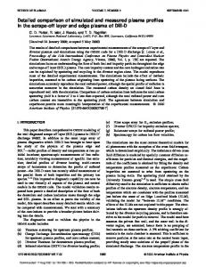
FIG. 1. A schematic representation of our bounded magnetosphere model.

these modes approaches zero as the wave number becomes larger. They also showed that, although the growth rate still has a maximum with respect to the flow speed, it now tends to zero only as the flow tends to infinity. This is in contrast to the unbounded modes containing a vortex sheet whose growth rate has a maximum, and then, above the upper cutoff speed, is identically zero. In other words, a bounded nonuniform magnetosphere has no upper cutoff speed. Physically, this corresponds to the fact that the energy can no longer simply propagate away from the magnetopause on the magnetosphere side as the waves are reflected by the inner boundary. Fujita et al.17 attributed these new properties to the nonuniform nature of the magnetosphere. They also looked at the solution of the dispersion relation for nonzero wave number perpendicular to the flow. They found that this gave rise to an enhancement in the frequencies found and that there was a cutoff flow-aligned wave number below which the modes were stable. Mann et al.18 considered a similar model to that of Fujita et al.,17 specifically a bounded uniform magnetosphere with zero plasma pressure connected to a field-free uniform flowing magnetosheath by a free sheet magnetopause 共as our model shown in Fig. 1 with P 1 ⫽0 and ␤⫽0兲. They showed that the same properties found by Fujita et al.17 were also found in a uniform magnetosphere and thus it is the fact that the magnetosphere is bounded 共rather than nonuniform兲 which has the most significant effect on the behavior of unstable surface modes at the magnetopause. Because of their model geometry, Mann et al.18 found that the fast surface mode is unstable for all nonzero flow speeds 共the lower cutoff speed is reduced to zero兲. This is because the stabilizing force of the magnetic tension is absent since the wave propagation does not bend the magnetic field. Mann et al.18 used an outgoing boundary condition in the magnetosheath that the group velocity of the waves there should be directed away from the magnetopause in the flowing frame of the magnetosheath. This replaces the condition of Fujita et al.17 that the modes should decay in amplitude away from the magnetopause. Besides the Mann et al.18 condition being more realistic than that of Fujita et al.17, it also allowed them to identify more complex behavior of the normal modes. In particular, this condition enabled Mann et al.18 to find cavity modes that decay in time and grow spatially in the magnetosheath for low flow speeds. These modes carry energy from the magnetosphere to the magnetosheath. They are

Kelvin-Helmholtz driven modes of the magnetosphere

4071

‘‘leaky’’ cavity/wave guide modes resulting from partial reflection and transmission of the magnetospheric waves at the magnetopause. The cavity modes were shown to become trapped for moderate flow speeds, which corresponds to the total internal reflection of the magnetospheric waves by a perfectly reflecting magnetopause. The modes become unstable or ‘‘over-reflected’’ for high flow speeds. In the case of over-reflected modes, energy from the magnetosheath flow is fed into the oscillations in the magnetosphere, increasing their amplitude. In this paper we consider a model similar to that of Mann et al.,18 however, we include finite plasma pressure in the magnetosphere and also consider modes propagating in an arbitrary direction. This allows us to study both fast and slow magnetoacoustic waves in the magnetosphere. We find that the onset of instability for all modes depends strongly upon the angle between the magnetic field and the wave vector 共and hence the angle between the wave vector and the magnetosheath flow兲 and show that the wave number selection found by Fujita et al.17 occurs for modes at all angles in a uniform magnetosphere model. In analyzing the modes that we find in our model we employ the concept of negative energy waves 共see Cairns;19 McKenzie;20 and also Joarder et al.21兲. We show that modes with group velocity directed away from the magnetopause in the moving frame of the magnetosheath may still feed energy from the magnetosheath into the magnetosphere. We find that the onset of instability of both fast cavity/wave guide and surface modes may be understood in terms of the coalescence of a positive energy mode with a negative energy mode. The structure of this paper is as follows: Sec. II presents our model, Sec. III gives the governing equations and discusses the boundary conditions, Sec. IV presents the concepts of wave energy and over-reflection and Sec. V discusses the results. In Sec. VI we derive a method for predicting the onset of instability for some of the modes, and Sec. VII compares our results to observations and summarizes our findings.

II. MODEL

We have used the ideal magnetohydrodynamic 共MHD兲 equations to consider a model for the modes generated in the magnetosphere by the flow discontinuity across the magnetopause. Our model consists of a bounded, uniform magnetosphere separated from an unbounded magnetosheath by a free magnetopause, which we assume to be infinitely thin. Figure 1 is a schematic diagram of our model. The magnetosphere is permeated by a constant magnetic field, B1 ⫽(0,0,B 1z ), which is tangential to the discontinuity, and has a finite pressure ( P 1 ) and density ( ␳ 01). It has an inner boundary which is taken to be perfectly reflecting, representing the refraction of MHD modes by the increasing Alfveń speed closer to the Earth. The inner boundary is taken to be at x⫽0 and the equilibrium magnetopause is at x⫽d. The magnetosheath is taken to be field-free with constant equilib-


4072


Mills, Wright, and Mann

rium pressure ( P 2 ) and density ( ␳ o2 ). The magnetosheath is flowing in the y-direction with a constant speed ( v o ). In order for this model to be in equilibrium we require total pressure balance across the magnetopause, given by P 1⫹

B 21 2␮o

⫽ P2 .

共1兲

Here, and throughout this paper, any quantity suffixed by a 1 defines a magnetospheric quantity, while a suffix 2 represents quantities in the magnetosheath. By choosing the ratio of the densities in the two regions ( ⑀ ⫽ ␳ o1 / ␳ o2 ) and the plasma beta 共␤兲 in the magnetosphere we can now derive a formula for the sound and Alfveń speeds in the magnetosphere in terms of the sound speed in the magnetosheath. The sound speed in the magnetosphere is given by

␤ 2 c s1 ⫽ c2 , ⑀ 共 1⫹ ␤ 兲 s2

共2兲

and the Alfveń speed by 2 ⫽ v a1

2 c2 . ␥⑀ 共 1⫹ ␤ 兲 s2

共3兲

III. EQUATIONS

We have normalized the ideal MHD equations with respect to the depth of the magnetosphere, d, and the equilibrium sound speed, c s2 , and density, ␳ o2 , in the magnetosheath. 共Gas pressure is normalized by the quantity ␥ P 2 , magnetic fields by 冑␥ P 2 ␮ o and time by d/c s2 .兲 Then we have added a small perturbation to each of our 共constant兲 equilibrium quantities and linearized the ideal MHD equations for a uniform medium, to give

␳o

冉

冉

冊

共5兲共6兲

冉

⳵ ⫹vo.ⵜ b⫽ 共 B.ⵜ 兲 u⫺B共 ⵜ.u兲 , ⳵t

冊

冉

⳵ ⳵ ⫹vo.ⵜ p⫽c s2 ⫹vo.ⵜ ␳ . ⳵t ⳵t

冊冉

共4兲

k⫽k y eˆy⫹k z eˆz,

共10兲

k⫽ 冑k 2y ⫹k z2 .

共11兲

and

We also define the angle between the tangential wave vector and the magnetospheric magnetic field in the y⫺z plane as

␣ ⫽arccos

冉冊

k.B1 . kB 1

共12兲

The relative directions of k, vo and B1 are illustrated in Fig. 2. We will be analyzing both the stable and unstable behavior of the system and so will assume that ␻ is a complex number ( ␻ ⫽ ␻ r ⫹i ␻ i ). Thus, ␻ r is considered to be the frequency and ␻ i is the growth 共or decay兲 rate of the amplitude of the oscillations. The total pressure perturbation in the magnetosphere (p T ⫽ p 1 ⫹B 1 b 1z ) can be shown to satisfy the second order differential equation d2pT dx 2

⫹m 21 p T ⫽0,

共13兲

where

⳵ ⫹vo.ⵜ ␳ ⫽ ␳ o ⵜ.u, ⳵t

ⵜ.b⫽0,

and

冊

⳵ ⵜ ⫹vo.ⵜ u⫽⫺ 共 p⫹ ␥ B.b兲 ⫹ 共 B.ⵜ 兲 b , ⳵t ␥

FIG. 2. A schematic diagram showing the relative directions of B1, the magnetic field in the magnetosphere, k, and vo, the magnetosheath velocity, in the y⫺z plane.

冊

共7兲

共8兲

Here, vo, B, P and ␳ o are the normalized equilibrium flow speed, magnetic field, pressure and density, respectively, while u, b, p and ␳ are the perturbations to these quantities, respectively. The coefficients of the perturbed quantities in these equations are now independent of t, y and z, so we may look for solutions of the form u共 x,y,z,t 兲 ⫽u共 x 兲 exp i 共 k y y⫹k z z⫺ ␻ t 兲 .

共9兲

Since the equations are normalized, the frequency, ␻, and the wave numbers, k y and k z , are variables of the normalized system. We define the tangential wave vector, k, such that

m 21 ⫽

2 兲共 ␻ 2 ⫺k 2 c 2f 兲共 ␻ 2 ⫺k 2 c slow 2 兲共 ␻ 2 ⫺k 2 c T2 兲共 c 2f ⫹c slow

,

共14兲

and m 1 is the wave number in the x-direction in the magnetosphere. When ␣⫽0, Eqs. 共13兲 and 共14兲 are equivalent to the equation for the motion of waves in a magnetic slab found by Roberts,22 however, it should be noted that in that paper, the wave equation is written as d 2 p T /dx 2 ⫺m R2 p T ⫽0, where the wave number is defined as m R2 ⫽⫺m 21 ( ␣ ⫽0). Here c f and c slow are the fast and slow magnetoacoustic speeds defined by 1 2 2 c 2f /slow⫽ 共共 v a1 ⫹c s1 兲 ⫹/ 2 2 2 2 2 2 ⫹c s1 c s1 cos2 ␣ 兲 , ⫺ 冑共 v a1 兲 ⫺4 v a1

共15兲

respectively, and c T is given by c T2 ⫽

2 c 2f c slow 2 c 2f ⫹c slow

⫽

2 2 c s1 v a1 2 2 ⫹c s1 v a1

cos2 ␣ .

共16兲




When ␣⫽0, c T is the tube speed for a magnetic slab defined by Roberts,22 and so c T may be thought of as the component of the tube speed along the propagation vector k. These three characteristic speeds satisfy the ordering 2 ⬍c 2f . c T2 ⬍c slow

共17兲

The perturbed pressure in the magnetosheath (p 2 ) satisfies the equation d2p2

⫹m 22 p 2 ⫽0.

dx 2

共18兲

Here m 2 is the x-component of the wave number in the magnetosheath given by m 22 ⫽

2 ␻ ⬘ 2⫺k 2 c s2 2 c s2

共19兲

.

We have defined ␻ ⬘ as the Doppler shifted frequency of the oscillations in the rest frame of the magnetosheath and it is related to ␻ by

␻ ⬘ ⫽ ␻ ⫺k v o sin ␣ .

共20兲

By assuming the equilibrium quantities are functions of x rather than constants we can obtain two first order ordinary differential equations which will enable us to specify the matching conditions across the magnetopause (x⫽1 in our normalized system兲. We must now retain terms in our governing equations that are concerned with the gradients of our equilibrium quantities. For example, the linearized momentum equation now becomes

␳o

冋冉

冊

⳵ ⫹vo.ⵜ u⫹ 共 u.ⵜ 兲 vo ⳵t

册

⫽⫺ⵜ 共 p To ⫹p T 兲 ⫹ 共 B.ⵜ 兲 b⫹ 共 b.ⵜ 兲 B,

共21兲

where p To ⫽p o ⫹B 2 /2, and our other equations are similarly modified. The equations are dp T 2 ⫽i ␳ o 共 x 兲关共 ␻ ⫺k v o 共 x 兲 sin ␣ 兲 2 ⫺k 2 v a1 共x兲 dx

再

ux d dx 共 ␻ ⫺k v o 共 x 兲 sin ␣ 兲 ⫽

共22兲

冎

2 ␳ o 共 x 兲共共 ␻ ⫺k v o 共 x 兲 sin␣ 兲 2 ⫺k 2 v a1 共 x 兲 cos2 ␣ 兲

pT , 共23兲

where 共共 ␻ ⫺k v o 共 x 兲 sin ␣ 兲

2

⫺k 2 c 2f 共 x 兲兲

2 共 c 2f 共 x 兲 ⫹c slow 共 x 兲兲

⫻

p T 共 x⫽1 兲 ⫽ p 2 共 x⫽1 兲 ,

共25兲

u x1 共 x⫽1 兲 u x2 共 x⫽1 兲 ⫽ . ␻ ␻⬘

共26兲

and

Equation 共25兲 corresponds to the continuity of total pressure across the magnetopause and Eq. 共26兲 implies that the displacement of the magnetopause is the same for both media 共so that there is no cavitation兲. These are the quantities that we would expect to be conserved at a discontinuous boundary.9,12,20 We require the boundary at x⫽0 to be totally reflecting, which may be imposed by the constraint u x1 共 x⫽0 兲 ⫽0.

2 共共 ␻ ⫺k v o 共 x 兲 sin ␣ 兲 2 ⫺k 2 c slow 共 x 兲兲

共共 ␻ ⫺k v o 共 x 兲 sin ␣ 兲 2 ⫺k 2 c T2 共 x 兲兲

.

共24兲

共27兲

Equation 共22兲 then implies the condition dpT 共 x⫽0 兲 ⫽0. dx

共28兲

Finally, we require the x-component of the group velocity of the perturbations in the rest frame of the magnetosheath to be directed away from the magnetopause. Because ␻ is complex, the wave numbers will also be complex. In this condition, therefore, we consider only the real part of the group velocity in the x-direction and require it to be positive in the rest frame of the magnetosheath. The dispersion relation for sound waves in the rest frame of the magnetosheath is 2 ␻ ⬘ 2⫽ 共 m 22 ⫹k 2 兲 c s2 ,

共29兲

where in the rest frame of the magnetosheath the waves oscillate with frequency ␻ ⬘ . The component of the group velocity of these waves in the x-direction is given by

⳵␻ ⬘ m 2 2 Re共 m 2 兲 ⫹iIm共 m 2 兲 2 ⫽ c ⫽ c . ⳵ m 2 ␻ ⬘ s2 Re共 ␻ ⬘ 兲 ⫹iIm共 ␻ ⬘ 兲 s2

共30兲

The real part of this component of the group velocity is Re共 v gx 兲 ⫽

im 2 共 x 兲

m 2共 x 兲 ⫽

We now assume that vo(x) and the other equilibrium quantities are step functions at the magnetopause, and integrate Eqs. 共22兲 and 共23兲 over the region 关1⫺␦,1⫹␦兴. Taking the limit as ␦→0, we find that the quantities p T and u x /( ␻ ⫺k v o sin ␣) must be continuous at the magnetopause. Hence, our matching conditions across the magnetopause are

v gx ⫽

ux ⫻cos2 ␣ 兴 , 共 ␻ ⫺k v o 共 x 兲 sin ␣ 兲

4073

Re共 ␻ ⬘ 兲 Re共 m 2 兲 ⫹Im共 ␻ ⬘ 兲 Im共 m 2 兲 Re共 ␻ ⬘ 兲 2 ⫹Im共 ␻ ⬘ 兲 2

2 c s2 .

共31兲

The condition that the real part of the group velocity in the x-direction is positive in the rest frame of the magnetosheath then becomes Re共 ␻ ⬘ 兲 Re共 m 2 兲 ⫹Im共 ␻ ⬘ 兲 Im共 m 2 兲 ⭓0.

共32兲

It can be shown that when this condition is satisfied the real part of the x-component of the phase speed, Re( v phx ) ⫽Re( ␻ ⬘ /(m 2 ))is always positive. Therefore this condition is equivalent to requiring that the phase speed in the magnetosheath rest frame is directed away from the magnetopause. In previous models 共e.g., Fujita et al.17兲 the condition that the amplitude of the observations decreases as x→⬁ has been


4074



used, which in our model would involve the condition that Im(m 2 )⬎0. The more general condition that we have used here allows us to find modes which decay in time and have a spatially growing nature in the magnetosheath 共leaky modes兲. We find that for low flows, most modes with positive phase speed in the magnetosheath are in fact leaky. In the case of stable modes ( ␻ i ⫽0), however, the wave number in the magnetosheath is purely imaginary, and so we have the condition that the modes must be evanescent, which in this special case gives our ‘‘outgoing’’ condition in the magnetosheath as Im共 m 2 兲 ⬎0.

共33兲

IV. THE THEORY OF NEGATIVE ENERGY WAVES

An important quantity in understanding the behavior of the instability at the magnetopause is the energy of the wave. Cairns19 showed that the energy per unit area of a stable hydrodynamic wave is given by

⳵D 2 1 A , E⫽ ␻ r 4 ⳵␻ r o

共35兲

where D is the dispersion relation of the waves and A o is the amplitude of the displacement of the fluid. We now show how this result is extended to magnetohydrodynamics 共see also Joarder et al.21兲. When the displacement of the magnetopause is given by

␩ ⫽A o exp i 共 k y y⫹k z z⫺ ␻ t 兲 , Combining the solutions to the wave equations 共13兲 and 共18兲 with the various boundary conditions yields the dispersion relation

冉

2 ␻ 2 ⫺k 2 v a1 cos 2 ␣ ⑀ m1

冊冉

冊

exp共 im 1 兲 ⫹exp共 ⫺im 1 兲 ␻ ⬘2 ⫺ ⫽0. exp共 im 1 兲 ⫺exp共 ⫺im 1 兲 m2 共34兲

When ␣⫽0, in the absence of flow, and considering only real ␻, this dispersion relation reduces to that in Roberts.22 The boundary condition at x⫽0 in our model without flow is equivalent to a sausage mode boundary condition in the center of the slab considered by Roberts, and so our model will yield only half the modes found in that paper. The other class of modes 共kink modes兲 could be generated by replacing Eqs. 共27兲 and 共28兲 with the condition p T (x⫽0)⫽du x1 /dx(x ⫽0)⫽0. Depending upon the sign of m 21 共i.e., by considering whether m 1 is real or imaginary兲, this equation describes both the body and surface modes found by Roberts. Allowing ␻ to be complex means that this dispersion relation describes not only purely oscillatory or evanescent modes, but also modes that have both oscillations and a background growth or decay in x. We have used a two-dimensional Newton-Raphson code, adapted from that in Ref. 23 to solve the dispersion relation numerically, yielding the complex eigenvalues ␻ for a given set of parameters 共k, ␣ and v o ). In order to maximize the efficiency of the code we have incorporated a backstepping routine to check that each iteration decreases the magnitude of the complex dispersion relation. The results of the code have been checked 共by taking the appropriate limits兲 qualitatively against the results in Roberts22 and Nakariakov and Roberts,24 and quantitatively against the results from Mann et al.18 We found that our code agreed with that of Mann et al.18 to at least 1 part in 106 . The code finds the roots ( ␻ ⫽ ␻ r ⫹i ␻ i ) such that the absolute value of both the real and imaginary parts of the dispersion relation and the calculated increment in the real and imaginary parts of the frequency are less than the value of ␦. In all cases ␦ ⬍10⫺6 , and in most cases, it is three or four orders of magnitude smaller.

共36兲

where A o is the amplitude of the oscillation, the linearized ideal MHD equations yield p T 共 x⫽1 兲 ⫽D 1 共 ␻ ,k 兲 ␩

共37兲

p 2 共 x⫽1 兲 ⫽D 2 共 ␻ ,k 兲 ␩ .

共38兲

and

We have defined D 1 共 ␻ ,k 兲 ⫽

2 cos2 ␣ 兲 cos m 1 ⫺ ␥ ␳ 1 共 ␻ 2 ⫺k 2 v a1

m1

,

共39兲

and D 2 共 ␻ ,k 兲 ⫽

⫺ ␥ ␳ 2 ␻ ⬘ 2sin m 1 . 兩 m 2兩

共40兲

Then, the work done per unit area in setting up the wave is found to satisfy Eq. 共35兲 with D defined so that D⫽⫾ 共 D 1 ⫺D 2 兲 .

共41兲

The sign of D is chosen such that the energy of the wave is always positive when there is no flow in the system. By looking at the sign of C⫽ ␻ r

⳵D , ⳵␻ r

共42兲

we are able to classify waves as having either positive or negative energy. The presence of a negative energy wave will reduce the energy of the system in the frame of reference being considered. Cairns19 showed that this expression for the energy of a mode can be used to explain the onset of some instabilities. In particular, he showed that the Kelvin-Helmholtz instability occurs when a positive energy wave ‘‘coalesces’’ with a negative energy wave, a result that we will apply later. The idea of the waves coalescing is used to describe the fact that the onset of instability occurs when the solutions for the two waves with opposite energy converge to the same value. After this point the waves are unstable and the boundary conditions will select only one of the complex roots, so the positive and negative energy modes are seen to ‘‘merge’’ into the same unstable solution. This type of instability is also classed as a reactive instability.




V. RESULTS A. Existence and classification of stable modes

We first examine the results that can be obtained using a purely real frequency ( ␻ ⫽ ␻ r ). With real ␻ , the sound waves in the magnetosheath satisfy the dispersion relation 2 , 共 ␻ r ⫺k v o sin ␣ 兲 2 ⫽ 共 m 22 ⫹k 2 兲 c s2

共43兲

which implies that m 22 is real. Thus m 2 is either purely real (m 22 ⬎0), implying propagating solutions in the magnetosheath, or purely imaginary (m 22 ⬍0), which gives evanescent solutions in the magnetosheath. Similarly, m 21 关as defined in Eq. 共14兲兴, is also real when ␻ i ⫽0, and hence m 1 is either purely real or imaginary. In the case where m 1 is purely real, the dispersion relation 关Eq. 共34兲兴 becomes

⑀

冉

2 ␻ r2 ⫺k 2 v a1

cos ␣ 2

im 1

冊

␻ r⬘ ⫽0, m2 2

cot m 1 ⫺

共44兲

and, when m 1 is purely imaginary, Eq. 共34兲 becomes

⑀

冉

2 ␻ r2 ⫺k 2 v a1

cos ␣ 2

in 1

冊

␻ r⬘ ⫽0, m2

共45兲

where we have defined m 1 ⫽in 1 . In both cases the first term of the equation is imaginary and, if m 2 is real the second term is real. Hence, we can see that both the first and second terms 共the real and imaginary parts of the equation兲 must be identically zero for the equations to be satisfied. This can only be true for specific values of v o and so, in general, there is no solution to the dispersion relation for m 22 ⬎0 共real m 2 ). If m 2 is imaginary, then the two terms may balance each other and need not be zero individually. Thus solutions for real ␻ may only occur when m 22 ⬍0 共i.e., m 2 is imaginary兲, and the modes must decay exponentially away from the magnetopause in the magnetosheath. Thus, any oscillatory part of the mode is trapped or contained within the magnetosphere. With this condition, Eq. 共43兲 may be rearranged to give

冉

␻r ⫺ v o sin ␣ k

冊

2 2 ⬍c s2 .

共46兲

This implies that either ␻ r /k⫺ v o sin ␣⬍cs2, or v o sin ␣ ⫺␻r /k⬍cs2, which together give the restriction on the phase speed for a stable mode: v o sin ␣ ⫺c s2 ⬍

␻r ⬍ v o sin ␣ ⫹c s2 . k

To include the effects of the magnetosphere and in order to classify our stable modes we need to examine the sign of m 21 when ␻ i ⫽0, see Roberts.22 We find that for m 21 ⬍0 we have evanescent modes in the magnetosphere 共surface modes兲 and for m 21 ⬎0 we have modes that oscillate within the magnetospheric cavity 共body, cavity or wave guide modes兲. The modes are then subdivided into fast and slow modes depending upon their nature in the magnetosphere. This distinction is also manifested in the phase speed of the modes. Modes with v ph⭐c slow are classified as slow modes, whereas those with v ph⬎c slow are fast modes. From Eqs. 共14兲 to 共17兲, we find that slow surface modes may exist for 0⬍ v ph⬍c T ,

共48兲

where v ph is the phase speed of the mode ( v ph⫽ ␻ r /k), and slow body modes may occur for c T ⬍ v ph⬍c slow .

共49兲

Fast surface modes are found to exist where

2

coth n 1 ⫹

4075

共47兲

With ␣⫽␲/2 this condition reduces to that of Mann et al.18 It is important to note that while this is a necessary condition for the existence of stable modes, it is not a sufficient one. That is, when a nonzero growth rate is included, it is still true that stable modes may only exist within the given range of phase speed; however, there may also exist unstable modes within that range. This condition is not a sufficient condition because it takes into account only the dispersion relation for sound waves in the magnetosheath 关Eq. 共43兲兴. The total dispersion relation 关Eq. 共34兲兴 also takes into account the conditions in the magnetosphere, and this will further restrict the region in which stable modes may occur.

c slow⬍ v ph⬍c f ,

共50兲

and fast cavity modes exist where v ph⬎c f .

共51兲

Taking v o ⫽0 and letting k→⬁, we find that the dispersion relation for surface modes 关Eq. 共45兲兴 becomes

⑀

2 ␻ r2 ⫺k 2 v a1 cos2 ␣ ␻ r⬘ 2 ⫹ ⫽0, n1 n2

共52兲

where n 2 ⫽im 2 . Assuming that as k→⬁, ␻ r /k→const, we can solve this equation to find the asymptotic value of the phase speed for the surface modes. We find that, when there is no flow in the magnetosheath, only slow surface modes may propagate for ␣⫽0 共when ⑀⫽0.192 and ␤⫽0.5 these modes have v ph⫽0.700). We will see later that in this case fast surface modes may only propagate as a result of a nonzero flow. So now, combining the above criteria with that for the existence of stable modes 关Eq. 共47兲兴, our full criteria for stable slow surface modes is that they may exist for phase speeds in the range max共 0,v o sin ␣ ⫺c s2 兲 ⬍ v ph⬍min共 c T , v o sin ␣ ⫹c s2 兲 ,

共53兲

where v o must satisfy v o sin ␣⫺cs2⬍cT so that the above inequality may be satisfied. Similarly, stable fast surface modes may exist for phase speeds such that max共 c slow , v o sin ␣ ⫺c s2 兲 ⬍ v ph⬍min共 c f , v o sin ␣ ⫹c s2 兲 , 共54兲 when v o is in the range c slow⫺c s2 ⬍ v o sin ␣⬍c f ⫹cs2. Stable slow body modes may exist for max共 c T , v o sin ␣ ⫺c s2 兲 ⬍ v ph⬍min共 c slow , v o sin ␣ ⫹c s2 兲 , 共55兲 where v o sin ␣⫺cs2⬍cslow . Finally, stable fast cavity modes may exist for max共 c f , v o sin ␣ ⫺c s2 兲 ⬍ v ph⬍ v o sin ␣ ⫹c s2 ,

共56兲

where v o sin ␣⫹cs2⬎c f .


4076


FIG. 3. The variation of the regions of phase speed 共given in units of c s2 ) where different mode types may exist with propagation angle ␣. Of the dotted lines, a is the magnetosheath sound speed (c s2 ), b is the tube speed 关 c T ( ␣ ⫽0) 兴 in the magnetosphere when ␣⫽0, c is the sound speed in the magnetosphere (c s1 ) and d is the Alfveń speed in the magnetosphere ( v a1 ). Of the solid curves, e is the lower cutoff for stable modes ( v ph⫽ v o sin ␣ ⫺cs2) and f is the corresponding upper cutoff ( v ph⫽ v o sin ␣⫹cs2), while the curves of the fast speed, c f , slow speed, c slow, and tube speed, c T are indicated by the arrows. Here as in all the following diagrams ␤⫽0.5, ␥⫽5/3 and ⑀⫽0.192, and in this case we have taken v o ⫽4.0.

Figure 3 shows the dependence of the regions where modes may exist on the angle ␣. For all the figures in this paper we have taken ␤⫽0.5, ␥⫽5/3 and ⑀⫽0.192, and in this case we have taken v o ⫽4.0. The negative sloping shading shows regions where the magnetosphere can support a body mode (m 21 ⬎0). The unshaded regions show the values of phase speed for which the magnetosphere may support a surface mode (m 21 ⬍0). The boundaries are calculated using c T , c f and c slow as outlined above 关Eqs. 共48兲 to 共51兲兴. The region with positive sloping shading is the region of phase speed within which the magnetosheath may support stable ( ␻ i ⫽0) modes, which are not growing or decaying in time 关Eq. 共47兲兴. All of the modes can be divided into fast and slow modes by the line v ph⫽c slow , above which fast modes propagate and below which slow modes may propagate. As ␣ increases, the regions where slow modes may exist diminish, until when ␣⫽␲/2 only fast modes may propagate. Where the region within which stable modes may propagate 共positive sloped shading between e and f兲 overlaps with the unshaded regions, the conditions for purely evanescent modes in both the magnetosheath and the magnetosphere are both satisfied and we may find stable surface modes. These are the regions defined by Eqs. 共53兲 and 共54兲. Similarly, the overlap between the positive and negative sloping indicate the regions for which stable body modes may propagate, defined in Eqs. 共55兲 and 共56兲. The effect of changing the flow speed is to change the gradient of the outline of the positively sloping shaded region. When ␣⫽0, the region where stable modes may exist is independent of the value of v o , and the region moves most rapidly with increasing v o when ␣⫽␲/2. When ␣⫽␲/2, we effectively have the case studied by Mann et al.,18 although they found only fast surface and cavity modes as they neglected plasma pressure in the magnetosphere. The condition for stable modes 关Eq. 共47兲兴 is merely a


FIG. 4. Fast surface mode 共a兲 phase velocities and 共b兲 growth rates as a function of k for ␣⫽␲/2. Here we have plots for v o ⫽1.0 共solid line兲, v o ⫽2.0 共dotted line兲, v o ⫽3.0 共dashed line兲, v o ⫽4.0 共dot-dashed line兲 and v o ⫽5.0 共triple dot-dashed line兲. The magnetospheric fast speed (c f ) is shown in 共a兲 by a horizontal dashed line.

necessary condition, not a sufficient one. Thus we should remember that we may have unstable modes within this region also. However, the behavior of the slow 共shown in Fig. 8兲 and fast stable body modes when v o sin ␣⫺cs2 ⬍cT and c f , respectively, is that the phase speed is confined between the upper and lower boundaries. For the slow body modes, the phase speed asymptotes toward the tube speed as k→0, whereas the phase speed of the fast mode asymptotes toward the fast speed as k→⬁. Thus, the phase speed of the mode remains in the region where stable modes may propagate even when v o sin ␣⫺cs2 becomes arbitrarily close to c T or c f , and so the phase speed always remains within the bounds and the modes may remain stable. Thus the slow body modes may become unstable only when v o sin ␣ ⫺c s2 ⬎c T ,

共57兲

and similarly, the fast body modes may become unstable when v o sin ␣ ⫺c s2 ⬎c f .

共58兲

B. The fast surface mode

First we will examine the behavior of the fast surface mode with changing k. Figure 4 shows the phase speed and growth rate of the mode for various flow speeds, v o . Here we have taken ␣⫽␲/2. We can see that for all nonzero flow speeds, both the phase speed and the growth rate tend to zero as k→0. With ␣⫽␲/2 we can see that the mode is unstable for all k. For low flow speeds, we find that the phase speed is always below the fast speed, and as k→⬁, ␻ i →⬁. For higher flow speeds, we find that the phase speed first exceeds the fast speed, has a maximum and tends back down to c f as k increases. Here, the growth rate also has a maximum at a finite value of k, and then tends to zero for large k. In order to understand these results better, we now look at the x-component of the wave numbers in the magnetosphere and magnetosheath (m 1 and m 2 , respectively兲. Figure 5 shows the real and imaginary components of these two wave numbers as functions of k. For the low flow speeds shown in Fig. 4 共the cases with v o ⬍4), the real and imaginary parts of both m 1 and m 2 increase in size linearly with k.




4077

FIG. 5. The real and imaginary parts of the x-component of the wave numbers in the magnetosphere 关共a兲 and 共b兲, respectively兴 and the magnetosheath 关共c兲 and 共d兲, respectively兴 as functions of k for the same values of v o as in Fig. 4. In 共a兲 the value ␲/2 is shown by a horizontal dashed line.

In both regions, the imaginary parts of the wave numbers increase more rapidly than the real parts, and for these flow speeds the mode is dominantly evanescent in the magnetosphere. These modes correspond to those in Fig. 4 that have unbounded growth rate ( ␻ i →⬁) as k→⬁. For the modes plotted in Fig. 4 which have bounded growth rate ( v o ⫽4,5), the imaginary parts of both m 1 and m 2 are bounded in k. The real part of m 1 approaches ␲/2 for large k and these modes are dominantly oscillatory in the magnetosphere. A value of ␲/2 for the wave number in the x-direction here, indicates that these modes have only a quarter of a wavelength of oscillation across the magnetosphere, whereas traditional cavity models may trap a minimum of half a wavelength. These modes display the feature that 兩 Re(m 2 ) 兩 →⬁ and Im(m 2 )→0 as k→⬁. Thus, for sufficiently high flow speeds the fast surface modes become oscillatory in the magnetosheath also, although they resemble trapped modes in the magnetosphere. We now investigate the dependence of the stability of the fast surface mode on the parameters v o and ␣. Figure 6

FIG. 6. A contour plot of the growth rate, ␻ i , plotted against v o and ␣ for the fast surface mode with k⫽2.0. The solid contours show regions of positive growth rate indicating unstable modes, the dotted lines are in regions of negative growth rate showing leaky mode. The region containing no contour lines is the region for which stable surface modes exist.

shows a contour plot of the growth rate against v o and ␣ for the fast surface mode with k⫽2.0. The solid lines indicate positive values of ␻ i , whilst the dotted lines are the negative values. Here, it is obvious that although the mode is unstable for any nonzero v o when ␣⫽␲/2, there is a nonzero lower cutoff speed for all lower values of ␣. As ␣ →0, the value of the cutoff tends to infinity, since propagation perpendicular to the flow does not ‘‘feel’’ the flow, (vo.ⵜ)⬅ivo.k→0. There is also an upper cutoff speed for the existence of leaky modes and this also tends to infinity for small ␣. The angle ␣ has two effects on the properties of the model that cause this change in stability. First, the flow speed is always multiplied by a factor of sin ␣, and so for small angles, the effect of the flow is very small. Second, the angle of propagation affects the magnetic forces that the background field exert on the wave. The tension force is (B1.ⵜ)b⬅i(k.B1)b. Thus when ␣⫽␲/2 共i.e., when k.B1⫽0), no magnetic tension force is created. Conversely, when the propagation vector has a component along the field line 共i.e., k.B1⫽0), the oscillations will tend to bend the field line, introducing magnetic tension forces which help to stabilize the system. Thus for a given flow, decreasing ␣ will decrease the effect of the flow and introduce stabilizing magnetic tension forces. Fujita et al.17 studied the effect of a nonzero k z on the frequency and growth rate of the oscillations. However, where we have fixed the value of k⫽ 冑k 2y ⫹k z2 and varied the value of the angle ␣, Fujita et al. fixed the value of k z and varied k y . In this case, increasing k y is equivalent to increasing both k and ␣ ⫽tan⫺1(ky /kz). They found that there was a lower cutoff in k y below which the modes are stable. We have looked at the dependence on k and ␣ separately, and our results indicate that the stability of the fast surface modes has very little dependence on k 共see also Fig. 7 below兲, but a strong dependence on ␣. Hence, the lower cutoff in k y found by Fujita et al. is more clearly expressed as a cutoff in ␣ in our model.


4078



FIG. 8. The dispersion diagram for slow surface modes when v o ⫽0 and ␣⫽0. Here we have shown both the forward and backward propagating modes. FIG. 7. The variation with flow speed, v o , of 共a兲 the phase speed, and 共b兲 the growth rate of the fast surface mode for k⫽2 共solid line兲, k⫽4 共dotted line兲 and k⫽6共dashed line兲. Here we have taken ␣⫽␲/4. The diamond in 共a兲 shows the predicted point of onset of instability when k⫽2 and the triple dot-dashed line in both shows the value of v o at this point. The region bounded by the horizontal lines and the diagonal lines is the potentially stable region 关Eq. 共54兲兴.

Finally, Fig. 7 shows the evolution of the fast surface mode with flow speed for various values of k and with ␣⫽␲/4. Here we see that the speed at the onset of instability of these modes has little dependence on k, and that while the modes are stable, the values of the phase speed are almost independent of k and the phase speed for the unstable modes also has little dependence on k. We can understand this by rearranging the dispersion relation for stable surface modes 关Eq. 共45兲兴 in terms of the phase speed, v ph , so that 2 2 ⑀ 共 v ph ⫺ v a1 cos2 ␣ 兲 N 2 coth共 N 1 k 兲 ⫹ 共 v ph⫺ v o sin ␣ 兲 2 N 1 ⫽0, 共59兲

where N 1 ⫽n 1 /k and N 2 ⫽n 2 /k. Now we can see that the only explicit dependence on k in the dispersion relation is within the coth function. Since this function is very close to unity for most values of N 1 k, the dispersion relation for stable surface modes is almost independent of k. As we will see in Sec. VI, the onset of instability may be predicted using this form of the dispersion relation. Thus, the onset of instability for fast surface modes will be almost independent of k. The growth rate of the unstable surface modes at first seems to increase linearly with k and this occurs for speeds at which the mode has unbounded growth rate as k→⬁. For higher speeds, the mode has wave number selection and here we can see that the growth rate is small for all k. The discontinuity in ␻ i occurs at the change over from unbounded to bounded growth rate. The change in behavior of the growth rate of the fast surface mode occurs approximately where the line v ph⫽ v o sin ␣⫺cs2 crosses the line v ph⫽c f . In other words, the growth rate becomes bounded when v oⲏ

c f ⫹c s2 , sin ␣

increases. Since the modes are purely evanescent in the magnetosphere for low v o , they are fairly insensitive to the inner boundary. Thus there will be negligible dispersion 共i.e., k dependence兲 of the stable fast surface modes and the phase speeds will be the same for any k. C. Slow surface modes

Now we examine the behavior of the slow surface mode. From Fig. 3 we see that, for all values of ␣ when v o ⫽0, the region of phase speed for which slow surface modes may exist 共i.e., v ph⬍c T ), is almost entirely within the region for which stable modes may exist ( v o sin ␣⫺cs2⬍vph ⬍ v o sin ␣⫹cs2). Figure 8 shows the phase speed of the slow surface mode as a function of k when v o ⫽0 and ␣⫽0. For small k the phase speed approaches c s2 , and as k increases, the phase speed rapidly approaches its asymptotic value, which in this case is v ph⫽0.700. This mode is stable for all k, which we can explain in the same way as we did for fast surface modes. The dispersion relation for evanescent modes 关Eq. 共59兲兴 has little dependence on k, and so we expect the character of the modes to be independent of k. We have also shown the slow surface wave propagating in the opposite direction, which when v o ⫽0 is a reflection of the mode with positive phase speed in the v ph⫽0 line. Figure 9 shows the variation of phase speed with angle, ␣, when v o ⫽0 and k⫽10. This phase speed will be the phase speed of the slow surface modes for almost all k at that particular ␣. As ␣ increases, the phase speed decreases, approaching zero at ␣⫽␲/2. The phase speed of the mode propagating backward is simply the negative of that shown in this case. The dot-dashed line shows the value of the tube

共60兲

which in this case 共␣⫽␲/4兲 means that the growth rate will be bounded for v o ⬇4.7. We can also see that, unlike models of an unbounded magnetosphere with a sheet magnetopause, there is no upper cutoff speed for the instability, although the growth rates reach has a maximum and then decreases towards zero as v o

FIG. 9. The variation of phase speed with angle for the slow surface mode when v o ⫽0 and k⫽10. The dot-dash lines shows the variation of the value of the tube speed, c T , with ␣.




4079

FIG. 12. The phase speed 共solid line兲 and growth rate 共dot-dashed line兲 of the unstable slow surface mode when v o ⫽3.3 and ␣⫽␲/6. FIG. 10. The phase speeds 共a兲 and growth rates 共b兲 of slow surface mode as v o changes. In 共a兲 the dashed line represents the stable fast surface mode, and in 共b兲, the dashed line shows the growth rate of the unstable mode formed by the coalescence of the two stable fast surface modes. In 共a兲 the dot-dash lines show the upper and lower boundaries of the region where stable modes may exist ( v o sin ␣⫹cs2 and v o sin ␣⫺cs2, respectively兲, and the dotted lines in ascending order show the tube speed, c T , the slow speed, c slow and the fast speed, c f . The diamonds mark the predicted points at which modes will coalesce. The left and right dotted lines in 共a兲 show the values of v o given by Eqs. 共62兲 and 共63兲, respectively.

speed, c T , as ␣ changes. We can see that the phase speed of the slow surface mode is always below c T when v o ⫽0. Now we investigate the development of the slow surface mode as v o increases. Figure 10 shows both the positive and negative modes as a function of v o when ␣⫽␲/6 and k ⫽10. As v o increases from zero, the phase speeds of both modes increase. As the phase speed of the upper mode approaches the tube speed c T , it flattens. The phase speed of the lower mode continues to increase, passing through zero, until the phase speeds of the two modes are the same. At this point the modes become unstable and our outgoing boundary condition 关Eq. 共32兲兴 selects only one of the two possible solutions. The phase speed of the unstable mode continues to increase and passes through the region where we would expect to find slow body modes (c T ⬍ v ph⬍c slow). However, the modes have a significant growth rate and remain dominantly evanescent in the magnetosphere 共see Fig. 11兲. The growth rate reaches a maximum and decreases back to zero when the phase speed is just above c slow . The modes are now stable fast surface modes, and once again we have two separate solutions. The phase speed of the lower solution decreases, tending to c slow as t→⬁. The mode becomes un-

stable when v o sin␣⬇cslow and has a small bounded growth rate. The upper mode has an increasing phase speed and eventually coalesces with the original stable fast body mode 共that has v ph⬎c slow for all v o , shown by a dashed line兲. These modes then become unstable, and the behavior of the resulting unstable mode is described in Sec. V B. The phase speed of the lower stable slow surface mode increases with the same gradient as v o sin ␣, so that its phase speed is v ph⫽⫺ v pho⫹ v o sin ␣ ,

共61兲

where v pho is the phase speed of the upper slow surface mode when v o ⫽0. The slow surface modes become unstable when the phase speed is close to the tube speed, c T , so we can approximate the flow speed at the onset of instability by v o⬇

c T ⫹ v pho . sin ␣

共62兲

Similarly, the modes become unstable again when the phase speed is close to the slow speed c slow and so we can approximate this by v o⬇

c slow⫹ v pho . sin ␣

共63兲

The values of v o predicted by Eqs. 共62兲 and 共63兲 are shown by the vertical dotted lines in Fig. 10. We can see that while this is not an accurate way of predicting the onset of instability and the point at which the modes restabilize, the values are at least reasonably close. The onset of instability can be more accurately predicted, and a method for this is detailed in Sec. VI. Finally, we look at the development of the unstable slow surface mode with k. Figure 12 shows the phase speed and growth rate of the mode when v o ⫽3.3 and ␣⫽␲/6 共close to the largest growth rate in Fig. 10兲. Here we can see that the phase speed varies little with k even when the mode is unstable; however, the growth rate increases with k and ␻ i →⬁ as k→⬁. Thus the unstable part of the slow surface mode has unbounded growth rate as k increases in the same way as the unstable fast surface mode. D. Slow body modes

FIG. 11. The real 共solid line兲 and imaginary 共dashed line兲 parts of the x-direction wave number in the magnetosphere, m 1 , as a function of v o for the lower slow surface mode shown in Fig. 10.

As we saw in Sec. V A, the range of phase speed for which slow cavity modes may exist depends very strongly on the value of ␣. Where the effect of the flow is greatest, the slow cavity modes are confined to a very small interval of


4080



very small and the imaginary part of the wave number in the magnetosphere will remain small compared to the real part, hence the character of the waves remains dominantly that of a trapped cavity mode. As k increases, ␻ i also increases, reaching a maximum 共which is much lower than the maximum growth rate for the globally oscillatory modes seen in Sec. V B兲 and then rapidly decreasing to zero. As the phase speed crosses the lower cutoff line, the modes become stable trapped slow cavity modes. From these results we can see that the slow cavity modes are never as fast growing as the fast modes or the slow surface mode and hence, we are much less likely to see them excited to a significant amplitude in the magnetosphere. FIG. 13. The dispersion diagram showing stable slow cavity modes when v o ⫽2 and ␣⫽␲/4.

phase speed close to zero. In order to examine the modes as fully as possible, we have chosen to look at modes with ␣⫽␲/4, where, for our given parameters, the slow cavity modes are stable when there is no flow. As detailed in Sec. V A, the slow cavity modes will only become unstable when the lower limit in Eq. 共55兲 changes from c T to v o sin ␣⫺cs2, and thus the slow cavity modes can only be unstable when c T ⫹c s2 , v o⬎ sin ␣

共64兲

so in this case the modes will be stable for all k when there is no flow in the magnetosheath. Figure 13 shows the form of the stable slow cavity modes. Next we look at the dispersion diagram for unstable slow cavity modes. Figure 14 shows the behavior of ␻ r /k and ␻ i for v o ⫽2.55 and ␣⫽␲/4. The upper and lower dashed lines mark the slow speed, c slow , and the tube speed, c T , respectively. The triple dot-dashed line shows the position of the lower cutoff for stable slow cavity modes from Eq. 共55兲, which in this case is v ph⫽ v o sin ␣⫺cs2. Here we see that the form of the phase speed is changed little from the stable case. For low k, the phase speed is below the lower stability cutoff, and the mode is unstable. The value of the growth rate is

E. Fast cavity modes

We saw in Sec. V A that stable fast cavity modes may exist when v o sin ␣⫹cs2⬎c f and they may have phase speeds within the range max共 c f , v o sin ␣ ⫺c s2 兲 ⬍ v ph⬍ v o sin ␣ ⫹c s2 .

共65兲

As explained in Sec. V A, the fast cavity modes will only be unstable if the lower limit of Eq. 共56兲 changes 共in this case from c f to v o sin ␣⫺cs2). Hence, the fast cavity modes will only be unstable if v o⬎

c f ⫹c s2 . sin ␣

共66兲

We may write the dispersion relation for stable cavity modes 关Eq. 共44兲兴 as tan共 m 1 兲 ⫽

⫽

2 cos2 ␣ 兲 n 2 共 ␻ 2 ⫺k 2 v a1

m 1 共 ␻ ⫺k v o sin ␣ 兲 2 2 n 2 共 ␻ 2 ⫺k 2 v a1 cos2 ␣ 兲

共 ␻ ⫺k v o sin ␣ 兲 2

⫻

冑

2 兲共 ␻ 2 ⫺k 2 c T2 兲共 c 2f ⫹c slow

2 兲共 ␻ 2 ⫺k 2 c 2f 兲共 ␻ 2 ⫺k 2 c slow

,

共67兲

where n 2 ⫽im 2 . Using this form of the dispersion relation and defining

FIG. 14. The phase speed 共solid line and left-hand axis兲 and growth rate 共dot-dashed lines and right-hand axis兲 as functions of k for slow cavity modes when v o ⬎(c T ⫹c s2 )/sin␣. Here v o ⫽2.55 and ␣⫽␲/4. 共The triple dotdashed line is the phase speed cutoff, below which modes are unstable.兲




FIG. 15. 共a兲 The dispersion diagram for the fast cavity modes in the case v o ⬎(c f ⫹c s2 )/sin ␣ 共in fact, here v o ⫽6.0 and ␣⫽␲/4兲. The predicted points of onset on instability 共derived in Sec. VI兲 are shown by diamonds, and the dotted lines mark the values of k at the onset. The upper and lower cutoffs and the fast speed are also shown. 共b兲 The growth rates as functions of k for the modes shown in 共a兲. The dotted lines again show the k value of the predicted onset of instability.

A 2⫽

m 21 k2

⫽

2 2 2 ⫺c 2f 兲共 v ph ⫺c slow 兲共 v ph 2 2 ⫺c T2 兲兲共 v ph 共 c 2f ⫹c slow

,

共68兲

we see that at the upper end of the range of phase speed where stable modes may exist ( v ph⫽ v o sin ␣⫹cs2), n 2 ⫽0 and therefore tan(m1)⬅tan(A(vph)k)⫽0. Thus the upper cutoff for stable fast body modes occurs when k⫽

n␲ . A 共 v o sin ␣ ⫹c s2 兲

共69兲

As k increases, the phase speed of the stable fast cavity modes tends to the fast speed, c f 共see for example Roberts22兲. When v o satisfies c f ⫺c s2 c f ⫹c s2 ⬍ v o⬍ , sin ␣ sin ␣

共70兲

共i.e., the flow is fast enough to allow stable cavity modes 关Eq. 共56兲兴, but not fast enough for those modes to become unstable 关Eq. 共66兲兴兲, stable fast cavity modes may propagate for all k greater than the cutoff defined in Eq. 共69兲. In Fig. 15 we show the dispersion diagram for the fast cavity modes when the flow speed is fast enough to allow the modes to become unstable 关as defined in Eq. 共66兲兴. We have used v o ⫽6.0 and ␣⫽␲/4. As well as the modes that we find when v o ⬍(c f ⫹c s2 )/sin ␣, we find that there are additional modes that begin at the lower cutoff 共given by v ph ⫽ v o sin ␣⫺cs2) and have phase speed increasing as k increases. The value of k at the lower extreme of the region in which stable modes may propagate is found by placing v ph ⫽ v o sin ␣⫺cs2 in the dispersion relation 关Eq. 共67兲兴. Noting that n 2 must be zero 共for a stable mode兲, we find that the value of k at the cutoff is n␲ . k⫽ A 共 v o sin ␣ ⫺c s2 兲

共71兲

Physically, these waves correspond to the fast modes that exist with negative phase speed when v o ⫽0. In the frame of the magnetosheath, these modes propagate against the flow 共and at the lower extreme they have phase speed ⫺c s2 in the

4081

frame of the magnetosheath兲, but once the flow is sufficiently high, the modes become oscillatory in the magnetosphere frame. As k increases, the phase speed of the upper mode branch decreases, whilst the phase speed of the lower mode branch increases until the two modes meet and coalesce. A fuller description of this is given in Sec. VI. For higher k beyond the point of coalescence, the modes are unstable. The phase speed decreases and asymptotically approaches c f for large k. The growth rate of the mode is, in most cases, bounded. The growth rate is of the same order as that of the unstable fast surface mode and so these modes will also be easily observed. However, as with the fast surface mode, the growth rate is not always bounded. The fast cavity modes have bounded growth for low v o 共above the minimum speed for instability兲. However, at the same speed at which the fast surface mode becomes globally oscillatory, the fundamental fast cavity mode starts to have an unbounded growth rate as k→⬁ and will become dominantly evanescent in the magnetosphere. Thus the ‘‘low v o ’’ surface and fundamental body mode exchange character as v o increases to being predominantly body and surface modes, respectively. Evidently the distinction between body and surface modes in a compressible plasma is not as clear as in an incompressible one. At some higher flow speed this new surface mode again becomes globally oscillatory and the second harmonic 共rather than the fundamental兲 fast cavity mode now develops an unbounded growth rate, and assumes a surface mode structure. Indeed, it would appear that for any nonzero flow, there will always be one mode whose growth rate increases without bound as k →⬁ and is predominantly a surface mode. However, these modes have large spatial decay in the magnetosphere and so are unlikely to be observed within the magnetospheric cavity. The development of a fast body mode as a function of v o is shown in Fig. 16. The mode is leaky for small v o with phase speed greater than that in the region where stable modes are possible. The mode remains leaky as the flow increases, even for some of the potentially stable region. However, farther into the region the mode becomes a stable fast cavity mode. Further increasing the flow, the mode becomes unstable. We again see that the mode is also unstable for some values of v o within the range of potentially stable phase speed, and we will develop a method for predicting the onset of the instability in the next section. 关The discontinuity in Im(m 2 ) is because of a branch cut in m 2 in the complex plane.兴 The ability of the magnetospheric cavity to excite, or even to trap waves, is strongly dependent on the flow speed in the magnetosheath.

VI. PREDICTION OF THE ONSET OF INSTABILITY

We have found that the onset of instability for slow cavity modes in our model is predicted exactly by the extremes of the region of phase speed for which stable modes may exist. However, this is not true for either the fast cavity or surface modes, and we now show how we may predict the exact position of onset of instability for these modes.


4082



FIG. 17. The form of F within the region of phase speed in which stable fast body modes may exist when v o ⫽5 and ␣⫽␲/4.

F 共 v ph兲 ⫽ ⑀

2 2 S 共 v ph兲共 v ph ⫺ v a1 cos2 ␣ 兲

A 共 v ph兲共 v ph⫺ v o sin ␣ 兲 2

S 2 共 v ph兲 ⫽⫺

m 22 k2

⫽

2 ⫺ 共 v ph⫺ v o sin ␣ 兲 2 c s2 2 c s2

共73兲

,

,

共74兲

and A is as defined in Eq. 共68兲. As explained in Sec. V A, the fast cavity modes only become unstable as k→⬁ when c f ⬍ v o sin ␣ ⫺c s2 ,

FIG. 16. 共a兲 The phase speed 共solid line兲 and growth rate 共dot-dashed line兲 as functions of v o for the fundamental fast cavity mode with k⫽3 and ␣⫽␲/4 共the upper branch in Fig. 15兲. The diamond represents the predicted point of the onset of the instability, and the dotted line shows the v o value at this point. The triple-dot-dashed lines show the positions of the upper and lower cutoffs of the region where stable modes may exist. The dashed lines indicate the values of v o between which the fast modes are stable for all k. 共b兲 The real 共solid line兲 and imaginary 共dot-dashed line兲 parts of the magnetosphere wave number of the mode, and 共c兲 the real 共solid line兲 and imaginary 共dot-dashed line兲 parts of the magnetosheath wave number.

A. Fast cavity modes

As we have seen from our results, the onset of instability for each fast mode occurs within the region of phase speed for which stable modes may exist. In order to examine the solutions more closely we have rewritten the dispersion relation for trapped cavity modes 共having ␻ i ⫽0) as D R ⫽0, where D R ⫽tan共 A 共 v ph兲 k 兲 ⫺F 共 v ph兲 , where

共72兲

共75兲

and, within the stable range given by Eq. 共47兲, both A and S are real. S is chosen to be positive to ensure spatial decay in the magnetosheath, and the sign of A is arbitrary, so we assume it to be positive 共if we took A negative, the dispersion relation we are solving would simply become ⫺D R ⫽0). Examining F within the region of phase speed for which stable modes may exist 关Eq. 共47兲兴 and where Eq. 共75兲 is satisfied, we see that it is singular at v ph⫽ v o sin ␣, and that F→0 as v ph→ v o sin ␣⫾cs2 共i.e., where S⫽0). Although F ⫽0 when v ph⫽ v a1 cos ␣, this does not occur within the range of phase speed we are considering as v a1 cos ␣⭐c f for all ␣. Figure 17 shows the form of F within this region when v o ⫽5 and ␣⫽␲/4. The function is shown both on a large and small scale to emphasize the behavior at the middle and end points of the region, respectively. In both plots the dotted lines represent the end points of the region where stable modes may occur, and the dot-dashed line represents the middle of the region where F is singular. Figure 18 shows F as a function of v ph with the function tan(Ak) over-plotted in a dashed line for various values of k. We see that for low k, the dashed line is almost straight, but as k increases the period of the tan function decreases, and the number of crossing points of the two functions 共corresponding to values of v ph where D R ⫽0) increases. From this we can see that there will be more stable roots of the dispersion relation as k increases, a fact which was borne out by our numerical solutions of the dispersion relation, see Fig. 15. Taking v ph⫽ ␺ 1 ⫽ v o sin ␣⫺cs2共so that F⫽0) and a given low value of k, we know that tan共 A 共 ␺ 1 兲 k 兲 ⬎0,

共76兲

and therefore D R ( ␺ 1 )⬎0.




4083

d dF , 共 tan共 Ak 兲兲 ⬎ d v ph d v ph

共78兲

the tan function will only encounter the curve of F at that one point and so there will be no double root. Differentiating the left-hand side of Eq. 共78兲, we get dA d k sec2 共 Ak 兲 , 共 tan共 Ak 兲兲 ⫽ d v ph d v ph

共79兲

and, since tan(Ak)⫽0 implies that Ak⫽n ␲ , and A and F are independent of k, we can use this to simplify Eq. 共69兲 so that our upper limit on the value of k at which a double root can occur is FIG. 18. The form of F within the region of phase speed in which stable fast body modes may exist when v o ⫽5 and ␣⫽␲/4, with the function tan(Ak) overplotted as dashed lines for various values of k.

Now we assume that the first value of the phase speed 共above the lower cutoff for the existence of stable modes v ph⫽ v o sin ␣⫺cs2) at which tan(Ak)→⬁ is at phase speed v ph⫽ ␺ 2 . In the first instance we will assume that ␺ 2 ⬍ v o sin ␣. At this point, we know that D R ( ␺ 2 )⬎0. The function D R is continuous in the range ( ␺ 1 , ␺ 2 ) and so there are three possibilities for the solutions of the dispersion relation within this range: 共i兲 Two real, distinct solutions of Eq. 共34兲; 共ii兲 No real solutions of the dispersion relation 关there will be two complex conjugate solutions, of which we will pick the one which satisfies Eq. 共32兲兴, or; 共iii兲 One real, ‘‘double’’ root of the equation 共i.e., a root that touches but does not cross the D R ⫽0 line兲. This must then be a turning point of the dispersion relation with respect to v ph and at this point

k⬎

dF d v ph

冒

dA d v ph

共80兲

evaluated at v ph⫽ v o sin ␣⫺cs2. Once k is above this limit the fast cavity modes will become unstable at exactly v ph ⫽ v o sin ␣⫺cs2, and the lower branch of each harmonic will not be apparent. Figure 15 includes the points 共marked by diamonds兲 that we have predicted for the onset of instability using a twodimensional 共2D兲 Newton method to solve the two equations. Here we have used a second order Taylor series approximation to find the value of the derivative, but the code still converges quickly to the double root. Similarly, if we fix k, we can solve the simultaneous Eqs. 共77兲 for v ph and v o 共or ␣兲 to predict the onset of the instability in terms of those variables. We show the predicted onset of instability in Fig. 16 by a diamond and the dotted line marks the v o value of this point. The predicted v o value agrees exactly with the value at which the instability occurs for our numerical results.

B. Surface modes

D R ⫽0

⳵DR and ⫽0. ⳵ v ph

共77兲

In fact, although F is not strictly continuous at v ph ⫽ v o sin ␣, the above analysis holds for all values of ␺ 2 ⬎ v o sin ␣⫺cs2 because F is always positive. Now, since we know from our numerical results 共see Fig. 15兲 that there are two real roots of the dispersion relation for low k, and at larger k these roots have become a single complex root 共chosen from the two possible complex roots by our outgoing condition in the magnetosheath兲, it follows that the transition must occur at a ‘‘double’’ real root. Thus, by solving the simultaneous equations given in Eq. 共77兲 for the variables k and v ph , we can numerically predict the onset of instability for these two fundamental modes. As k increases, new branches of the tan function encounter the curve of F for low v ph . Thus successively higher harmonic modes have double roots at which they go unstable. However, this will not be the case for all higher k. The lower branch of each harmonic first appears at a value of k such that tan(Ak)⫽0 when v ph ⫽ v o sin ␣⫺cs2. However, if at that value of k

The dispersion relation for stable surface modes 关Eq. 共59兲兴 may be written as 2 2 D S ⫽N 1 共 v ph⫺ v o sin ␣ 兲 2 tanh共 N 1 k 兲 ⫹ ⑀ N 2 共 v ph ⫺ v a1

⫻cos2 ␣ 兲 ⫽0, N 21 ⫽⫺m 21 /k 2

共81兲 N 22 ⫽⫺m 22 /k 2 .

and By analyzing the where two terms of the equation in a similar way to that used for the dispersion relation for fast cavity modes, we may again show that the onset of instability may be predicted by simultaneously solving the equations D S ⫽0,

and

⳵DS ⫽0, ⳵ v ph

共82兲

for v ph and either of v o and ␣. Figure 7 includes the point at which instability is predicted by this method when k⫽2 as shown by a diamond. The vertical three dot-dash line shows the predicted value of v o and is in excellent agreement with the onset of instability given by our numerical solution. Similarly, in Fig. 10 we have plotted the points that satisfy Eqs. 共82兲 as diamonds. The points predict excellently the


4084



FIG. 20. A summary of the properties of the slow cavity modes.

C⫽ v ph

FIG. 19. 共a兲 The dispersion diagram showing the upper 共solid line兲 and lower 共dot-dashed line兲 fundamental fast cavity modes when v o ⫽5.0 and ␣⫽␲/2. The diamond shows the predicted point of coalescence and onset of instability and the dotted line shows the k value of this point. 共b兲 A plot showing C 共which is proportional to the energy of the wave兲 as a function of k for the stable part of the two modes, and 共c兲 an enlargement of the area around the point of coalescence. The dotted line shows the predicted k value of the coalescence.

points where the stable surface modes coalesce and become unstable, as well as the point where the unstable mode becomes stable and splits into two modes. In Sec. V B we saw that the onset on instability of the fast surface modes is almost independent of k 共see Fig. 7兲. Examining Eq. 共81兲 we can see that the only explicit dependence on k when the dispersion relation is written in terms of the phase speed is within the function coth(N1k). This function only varies significantly when N 1 k is small and is close to unity for N 1 kⲏ1. Thus the double roots of the dispersion relation will vary little as k varies.

dD R . d v ph

共83兲

Figure 19 shows the coalescence of the fundamental fast cavity modes in the top diagram, again with the predicted onset of instability shown by a diamond. The lower diagram shows the value of C for the two modes while they are both stable. We can see that the upper mode has positive energy, whilst the lower has negative energy. As k increases toward the value at which instability occurs 共represented here by a vertical dotted line兲, the magnitude of the energy of both modes tends toward zero. Thus this instability occurs when a positive and negative energy wave coalesce, and the mathematical analysis above identifies the point at which C⫽0 and the two different energy waves meet. In Fig. 10 the slow surface mode that had negative phase speed when v o ⫽0 becomes a negative energy wave when the phase speed becomes positive, and so the onset of instability of the slow surface mode also corresponds to the coalescence of a negative energy wave with a positive energy wave. Southwood12 showed that the points of marginal stability for the shear flow discontinuity of an unbounded magnetosphere 共with both magnetic field and plasma pressure on both sides of the boundary兲 are given where both R 1 共 x 1 兲 ⫽⫺R 2 共 x 2 兲

共84兲

dR 1 dR 2 ⫽␰2 dx 1 dx 2

共85兲

and C. The onset of instability and the energy of the waves

Referring back to our definition of the wave energy of the stable modes 关Eqs. 共35兲 and 共42兲兴, we can show that, for given values of k, v o and ␣, C can be rewritten as

␰1

are satisfied. Here x 1 and x 2 are the phase speeds in the rest frames of the two fluids 共each normalized to the Alfveń




4085

FIG. 21. A summary of the properties of the fast cavity modes.

speed of that fluid兲 and R 1 and R 2 are the dispersion relations for each side of the boundary. ␰ 1 is defined such that

␰ j⫽

␻i , kvaj

共86兲

where j⫽1,2. We can show, by replacing Southwood’s normalizations with ours, that these conditions are equivalent to our conditions for the onset of instability, given in Eq. 共77兲. VII. DISCUSSION AND CONCLUSIONS

In comparison with wave guide mode models 共e.g., Wright25兲, which assume a perfectly reflecting magnetopause, we have looked at the trapping and excitation of cavity modes when the magnetopause is taken to be a free boundary. We have found that whether the magnetospheric cavity traps or excites modes is highly dependent on the value of v o 共the speed of the flow in the magnetosheath兲. The flow around the magnetopause has a stagnation point at the nose of the magnetosphere and then accelerates approaching the speed of the upstream solar wind flow along the flanks 共see Spreiter and Stahara26兲. Our model has shown that for low flow speeds the cavity modes are leaky, for moderate flows they become trapped and for high flow speeds they become unstable and energy from the magnetosheath flow is fed into the magnetosphere, increasing the amplitude of the body modes. More specifically, the trapping of fast cavity

modes occurs for values of the flow speed such that v o sin ␣⬎c f ⫺cs2, while slow cavity modes are trapped when v o sin ␣⬎cslow⫺c s2 . Excitation of fast and slow cavity modes occurs when v o sin ␣⬎c f ⫹cs2 and v o sin ␣⬎cT⫹cs2, respectively. The form of the flow around the magnetosphere is such that modes are most likely to be trapped or excited on the flanks and it is in this region that Pc5 oscillations are observed to be present almost continuously. On the flanks it has also been observed that there is a strong correlation between Pc5 wave power and the speed of the solar wind flow 共and hence the speed of the flow along the flanks兲. Although slow cavity modes may be trapped even in conditions of zero flow 共e.g., when ␣⫽␲/4兲 and excited for small values of v o , the growth rates of these modes are three orders of magnitude smaller than the growth rates of both the fast body and surface modes 共when they display wave number selection兲. Also, the maximum growth rate of the slow cavity modes occurs for values of v o close to the onset of instability. Hence we can conclude that slow cavity modes are unlikely to be excited to a sufficient amplitude to be easily observed. Since the trapping of fast cavity modes occurs for v o ⬎(c f ⫺c s2 )/sin ␣ and these modes are excited for v o ⬎(c f ⫹c s2 )/sin ␣, we can see that fast cavity modes will be most easily trapped or excited for values of ␣ close to ␲/2 共i.e., those modes propagating parallel or quasiparallel to the flow


4086



FIG. 23. A summary of the properties of the fast surface modes. FIG. 22. A summary of the properties of the slow surface modes.

in the magnetosheath兲. Using some typical values for the various parameters we get v a1 ⬇400⫺500 and c s2 ⬇120 km/s 共see Fujita et al.,17 and also Mann et al.18兲, we find that quasiparallel propagating fast cavity modes will be trapped for solar wind speeds of v sw⬎300⫺400, and excited when v sw ⬎500⫺600 km/s. This is in excellent agreement with Engebretson et al.,1 who observed that Pc5 waves on the dawn flank have a much increased power index for v sw ⬎500 km/s. Fast cavity modes propagating obliquely to the magnetosheath flow will need significantly higher flow speeds to be excited or even trapped. Thus, observable Pc5 waves on the magnetospheric flanks may be expected to propagate quasiparallel to the flow in the magnetosheath. The almost continuous observation of Pc5 oscillations may be explained by the fact that wave trapping will occur for normal solar wind conditions. Above the threshold speed for instability of fast cavity modes we have found negative energy waves. These solutions represent modes that propagate in the negative y-direction 共i.e., sunward兲 when there is no flow. The onset of instability of the fast modes is found to occur when the dispersion curves of positive and negative energy waves meet, and at this point the wave energy is zero. The behavior of the slow cavity modes is summarized in flow chart form in Fig. 20. The slow cavity modes are first unstable for low k, as that is where they have lower phase speed, whereas the phase speed of the fast cavity modes 共the properties of which are summarized in Fig. 21兲 decreases with increasing k, and so these modes are first unstable for high k. The criterion for the onset of instability for fast cavity modes changes for high k 关defined by Eq. 共80兲兴 to occurring where v ph⫽ v o sin ␣⫺cs2. For any given value of ␣, all the fast cavity modes will be unstable for higher values of k once v o sin ␣⬎c f ⫹cs2. Fujita et al.17 found that the fast surface mode displays azimuthal wave number selection 共a maximum value of ␻ i for a finite value of k兲 for flow speeds above a threshold and

claimed this was a result of their nonuniform magnetosphere. We have shown that this behavior is also true for the case of a uniform magnetosphere and that the fast and slow cavity modes also display wave number selection. Fast and slow surface modes also exist in the magnetosphere. The behavior of the slow surface modes is summarized in Fig. 22. The slow surface modes become unstable for relatively low flow speeds; however, they restabilize and become fast surface modes for higher flow speeds. The upper of these surface modes coalesces with the original fast surface mode and becomes unstable. The growth rate of these modes is unbounded as k increases. The onset of instability of the fast surface modes occurs for decreasing v o as ␣ increases and is almost independent of k; when stable, these are fast surface modes decaying away from both sides of the magnetospheric boundary. For low flow speeds the unstable modes are predominantly evanescent in the magnetosphere, but for speeds above v o sin ␣ⲏc f ⫹cs2 the modes become globally oscillatory in the magnetosphere and display wave number selection. The behavior of the fast surface modes is summarized in Fig. 23. Using a free boundary allows the generation of quarter wavelength modes within the magnetospheric cavity. This is a feature not found in the traditional cavity mode models and may explain the lowest observed frequencies found in observations. Nonlinear effects have been shown to be important in the evolution of unstable surface modes at the magnetopause both through observations and numerical simulations.14,27 However, unstable body/wave guide modes have only recently received attention and have proved elusive in the data.28,29 We have considered the linear evolution of unstable modes in order to classify the criteria for the onset of instability and to compare the relative sizes of linear growth rates for the various types of modes. Nonlinear simulations of the growth of these modes would help to clarify their evolution.



ACKNOWLEDGMENTS


4087

A. Miura, J. Geophys. Res. 97, 10655 共1992兲. A. D. M. Walker, Planet. Space Sci. 29, 293 共1981兲. 16 A. Miura and P. L. Pritchett, J. Geophys. Res. 87, 7431 共1982兲. 17 S. Fujita, K.-H. Glassmeier, and K. Kamida, J. Geophys. Res. 101, 27317 共1996兲. 18 I. R. Mann, A. N. Wright, K. J. Mills, and V. M. Nakariakov, J. Geophys. Res. 104, 333 共1999兲. 19 R. A. Cairns, J. Fluid Mech. 8, 1 共1979兲. 20 J. F. McKenzie, Planet Space Sci. 18, 1 共1970兲. 21 P. S. Joarder, V. M. Nakariakov, and B. Roberts, Sol. Phys. 176, 285 共1997兲. 22 B. Roberts, Sol. Phys. 69, 39 共1981兲. 23 W. H. Press, S. A. Teukolsky, W. T. Vetterling, and B. P. Flannery, Numerical Recipes in Fortran 2nd ed. 共Cambridge University Press, Cambridge, 1992兲. 24 V. M. Nakariakov and B. Roberts, Sol. Phys. 159, 213 共1995兲. 25 A. N. Wright, J. Geophys. Res. 99, 159 共1994兲. 26 J. R. Spreiter and S. S. Stahara, J. Geophys. Res. 85, 6769 共1980兲. 27 J. R. Manuel and J. C. Samson, J. Geophys. Res. 98, 17367 共1993兲. 28 W. Allan, A. N. Wright, and D. R. McDiarmid, J. Geophys. Res. 102, 14407 共1997兲. 29 B. J. Anderson and M. J. Engebretson, J. Geophys. Res. 102, 14407 共1997兲. 14 15

K.J.M. was supported by a PPARC Research Studentship, A.N.W. was supported by a PPARC Advanced Fellowship and IRM was supported by a PPARC Fellowship. 1

M. Engebretson, K.-H. Glassmeier, M. Stellmacher, W. J. Hughes, and H. Luh, J. Geophys. Res. 103, 26271 共1998兲. 2 D. J. Southwood, Planet. Space Sci. 22, 483 共1974兲. 3 L. Chen and A. Haseagawa, J. Geophys. Res. 79, 1024 共1974兲. 4 L. Chen and A. Hasegawa, J. Geophys. Res. 79, 1033 共1974兲. 5 M. G. Kivelson, J. Etcheto, and J. G. Trotignon, J. Geophys. Res. 89, 9851 共1984兲. 6 M. G. Kivelson and D. J. Southwood, Geophys. Res. Lett. 12, 49 共1985兲. 7 M. G. Kivelson and D. J. Southwood, J. Geophys. Res. 91, 4345 共1986兲. 8 J. W. Dungey, ‘‘Electrodynamics of the outer atmosphere,’’ in Proceedings of the Ionosphere 共Physical Society of London, London, 1955兲, p. 25. 9 S. Chandrasekhar, Hydrodynamic and Hydromagnetic Stability 共Oxford University Press, New York, 1961兲, p. 482. 10 A. K. Sen, Phys. Fluids 7, 1293 共1964兲. 11 J. A. Fejer, J. Fluid Mech. 7, 499 共1964兲. 12 D. J. Southwood, Planet. Space Sci. 16, 587 共1968兲. 13 Z. Y. Pu and M. G. Kivelson, J. Geophys. Res. 88, 841 共1983兲.
