Design of an Unmanned Ground Vehicle, Bearcat III, Theory and Practice • • • • • • • • • • • • • • • • •
• • • • • • • • • • • • • •
Masoud Ghaffari,* Souma M. Alhaj Ali,† Vidyasagar Murthy, Xiaoqun Liao, Justin Gaylor, and Ernest L. Hall
Center for Robotics Research Department of Mechanical, Industrial and Nuclear Engineering University of Cincinnati Cincinnati, Ohio 45221-0072 e-mail:
[email protected]
Received 23 March 2004; accepted 23 March 2004
The purpose of this paper is to describe the design and implementation of an unmanned ground vehicle, called the Bearcat III, named after the University of Cincinnati mascot. The Bearcat III is an electric powered, three-wheeled vehicle that was designed for the Intelligent Ground Vehicle Competition and has been tested in the contest for 5 years. The dynamic model, control system, and design of the sensory systems are described. For the autonomous challenge line following, obstacle detection and pothole avoidance are required. Line following is accomplished with a dual camera system and video tracker. Obstacle detection is accomplished with either a rotating ultrasound or laser scanner. Pothole detection is implemented with a video frame grabber. For the navigation challenge waypoint following and obstacle detection are required. The waypoint navigation is implemented with a global positioning system. The Bearcat III has provided an educational test bed for not only the contest requirements but also other studies in developing artificial intelligence algorithms such as adaptive learning, creative control, automatic calibration, and internet-based control. The significance of this effort is in helping engineering and technology students understand the transition from theory to practice. © 2004 Wiley Periodicals, Inc.
1. INTRODUCTION Robot design generally falls into two categories: fixed industrial robots and mobile robots.1,2 Unmanned *To whom all correspondence should be addressed. † Also at Industrial Engineering Department, Hashemite University, B. O. Box: 150459, Zerka 13115 Jordan.
ground vehicles, UGVs, are a group of mobile robots with great promising potentials for the future. Space exploration,3,4 material handling,5 transportation, medical transport of food and patients and future combat vehicles6 are areas that traditionally have been emphasized and the laboratory results are beginning to find application in the real world.
Journal of Robotic Systems 21(9), 471–480 (2004) © 2004 Wiley Periodicals, Inc. Published online in Wiley InterScience (www.interscience.wiley.com). • DOI: 10.1002/rob.20027
472
•
Journal of Robotic Systems—2004
kinematic and dynamic model of Bearcat III is described. Section 3 describes the sensory systems with emphasis on line following: obstacle avoidance and waypoint navigation sensors. Sections 4 and 5 outline the performance prediction and the results. Figure 1. Major functional subsystems.
2. DESIGN A power source, manipulator, control and sensory systems are the basic elements of any UGV. This paper mainly deals with the dynamic control model and sensory systems design of an unmanned ground vehicle robot, the Bearcat III. In addition to those described in this paper, this robot has also been used to study internet-based control,7 automatic calibration,8 and creative control.9 The Bearcat III is an interactive and intelligent unmanned ground vehicle designed to serve in unstructured environments such as those encountered in the Intelligent Ground Vehicle Competition (IGVC), a contest which provides real world challenges. The Bearcat III was designed to perform all the tasks and obey all the rules required for this contest; however, we have found that continual improvement is necessary because of changing contest rules and technical innovations. This paper is organized as follows. Section 2 describes the overall block diagram of the system including the sensors and mechanical system. Then the
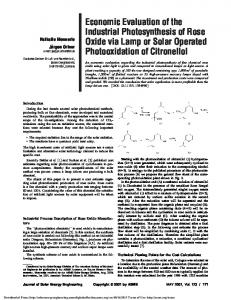
2.1. Design Process The design approach followed the Kaizen philosophy of continuous improvement.10 Our progress, through several sessions of brainstorming, always resulted in improvements of the design. 2.2. Enhanced System Diagram The major functional subsystems are shown in Figure 1. The control block diagram of the system is shown in Figure 2. 2.3. Mechanical System The Bearcat III was designed to be an outdoor vehicle able to carry a payload of at least 20 pounds. Optimal design was attempted using proper design practices and tools during the basic design. CAD software such as AutoCAD™ R14 and IDEAS™ Master series 7.0 were used in the final analysis phase for stress and
Figure 2. Bearcat III sensory block diagram.
Ghaffari et al.: Unmanned Ground Vehicle, Bearcat III
•
473
where v t ,v n , can be defined in terms of the angular velocity of the robot left wheel l and the angular velocity of the robot right wheel r as follows:11,12
冋册
vt vn ⫽ w
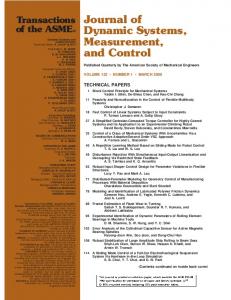
Figure 3. Mechanical design.
er 2d
⫺er 2d
r 2d
⫺r 2d
冋 册
l . r
(2)
冋册 冋
cos x˙ y˙ ⫽ sin ˙ 0
e sin ⫺e cos 1
册冋 册
vt .
(3)
The nonholonomic constraint can be obtained directly from Eq. (3) as11,12
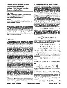
2.4. Dynamic Model For the Bearcat III robot, a kinematic and dynamic model was derived using the Newton–Euler method.11–14 Bearcat III structure and dynamic analysis are shown in Figure 4. According to Figure 4, the kinematic model with respect to the robot center of gravity [point C in Figure 4(a)] can be described as follows:11,12
冋册 冋
r 2
However, Eq. (1) can be simplified by utilizing that v n ⫽e as follows:11,12
load analysis. The robot’s frame is constructed of 80/ 20™ aluminum extrusions, joining plates and T-nuts. Figure 3 shows the frame assembly view of the mechanical system.
cos x˙ y˙ ⫽ sin ˙ 0
冋 册 r 2
sin
0
⫺cos
0
0
1
册冋 册
vt vn ,
(1)
x˙ sin ⫺y˙ cos ⫽ e.
(4)
For the center of the wheel axes [point E in Figure 4(a)] e⫽0 and hence Eq. (4) reduces to11,12 x˙ sin ⫺y˙ cos ⫽0.
(5)
This means that there is no motion in the direction of the wheel axis.
Figure 4. Robot dynamic analysis (ref. 11). (a) Robot structure. (b) Dynamic analysis for the right wheel. (c) Dynamic analysis for the robot.
474
•
Journal of Robotic Systems—2004
Another constraint for the kinematic model comes from the inertial structure of the robot where the robot’s path cannot exceed the minimum turning radius or the maximum curvature:11,12
⭓R min imum
or
k⭐K max imum .
(6)
From Figure 4(b), the Newton–Euler equation for the right wheel can be described as11,12
wheel by the rest of the robot; f r is the friction force between the right wheel and the ground; m w is the mass of the wheel; r is the torque acting on the right wheel provided by the right motor; r is the radius of the wheel; and J w is the inertia of the wheel. Note that the Coriolis part had been deleted since it is negligible due to the fact that the wheel inertia is much smaller than the robot inertia. The dynamic model of the robot can be defined as11,12
F r ⫺f r ⫽m w x¨ r , (7)
M 共 兲 ¨ ⫹J 共 , ˙ 兲 ˙ ⫹F⫽ ,
r ⫺F r •r⫽J w ˙ r , where F r is the reaction force applied to the right
M共 兲⫽
冋
J 共 , ˙ 兲 ⫽
F⫽
冋
where
共 mr 2 cos ⫹2J 0 cos 兲 2r
共 mr 2 sin ⫹2J 0 sin 兲 2r
共 mr 2 ed sin2 ⫺mr 2 ed sin cos ⫹J c r 2 ⫹2J 0 d 2 兲 2rd
共 mr 2 cos ⫹2J 0 cos 兲 2r
共 mr 2 sin ⫹2J 0 sin 兲 2r
共 mr 2 ed sin2 ⫺mr 2 ed sin cos ⫺J c r 2 ⫺2J 0 d 2 兲 2rd
⫺J 0 ˙ sin r
J 0 ˙ cos r
⫺mre ˙ cos 共 sin ⫹cos 兲 2
⫺J 0 ˙ sin r
J 0 ˙ cos r
⫺mre ˙ cos 共 sin ⫹cos 兲 2
冋 册 ⫺f n er d
⫺f n er d
,
⫽
冋册
r , l
(8)
册
册
,
,
冋册
xc ⫽ yE .
To customize the dynamic model for the Bearcat III, we need to substitute the values for m,r,J 0 ,e,d,J c ,f n in Eq. (8). According to Figure 4 for Bearcat III, m ⫽306.18 kg, r⫽0.2095 m, e⫽0.338 m, d⫽0.432 m, and J 0 ,J c ,f n need to be calculated. The value of the frictional coefficient between the ground and the wheel depends on the type of surface of the ground; for grass, 0.6 is common, while for concrete 0.9 is usually used. Bearcat III usually moves on grass, therefore, 0.6 was used in the calculations. Substituting the parameters for Bearcat III into the normal force equation f n ⫽ ( 31 mg⫹m w g), f n is calculated to be 629.45 N.12
The moment of inertia for the robot wheel is calculated as follows:12 2 2 2 J w ⫽ 21 m t 共 r te ⫺r ti2 兲 ⫹ 21 m r 共 r re ⫺r ri 兲 ⫽0.055 kgm2 .
(9) Substituting the value of J w from Eq. (9) for Bearcat III, J 0 is calculated to be 0.274 kgm2 . For more details, please refer to ref. 12. Substituting these values into Eq. (8), the Bearcat III dynamic model is12 M B 共 兲 ¨ ⫹J B 共 , ˙ 兲 ˙ ⫹G B 共 , ˙ , ¨ 兲 ⫽ , where
(10)
Ghaffari et al.: Unmanned Ground Vehicle, Bearcat III
冋册
xc ⫽ yc , M B共 兲 ⫽
⫽
冋
J B 共 , ˙ 兲 ⫽
r , l 33.454 sin
10.866 sin2 ⫺10.866 sin cos ⫹11.014
33.454 cos
33.454 sin
10.866 sin2 ⫺10.866 sin cos ⫺11.014
⫺1.305˙ sin
1.305˙ cos
⫺10.866˙ cos 共 sin ⫹cos 兲
⫺1.305˙ sin
1.305˙ cos
⫺10.866˙ cos 共 sin ⫹cos 兲
G B 共 , ˙ , ¨ 兲 ⫽
冋
475
冋册
33.454 cos
冋
•
册
册
,
,
册
11.308˙ 2 sin2 ⫺0.441˙ 2 cos2 ⫺11.308¨ sin cos ⫺103.422 . 11.308˙ 2 sin2 ⫺0.441˙ 2 cos2 ⫺11.308¨ sin cos ⫺103.422
3. SENSORY SYSTEMS 3.1. Autonomous Challenge Line Following and Obstacle Detection The autonomous challenge requires that the Bearcat III negotiate through an outdoor obstacle course in a prescribed time while staying within the 5 mph speed limit, traversing ramps with 10% incline, and avoiding both physical obstacles and painted potholes on the track.
right or left. If the track is lost from one side, then the central controller, through a video switch, changes to the other camera. In order to obtain accurate information about the position of the line with respect to the centroid of the robot, the distance and the angle of the line with respect to the centroid of the robot has to be known. When the robot is run in its auto-mode, two I-Scan windows are formed at the top and bottom of the image screen as shown in Figure 5. The centroids are shown as points (x 1 ,y 1 ) and (x 2 ,y 2 ) in Figure 6. The angle and distance of the line to the robot are determined.
3.2. Vision System The Bearcat’s vision system for the autonomous challenge comprises three cameras, two for line following and one for pothole detection. The vision system for line following uses 2 CCD cameras and an image tracking device (I-Scan™) for the front end processing of the images captured by the cameras. The I-Scan™ tracker processes the image of the line. The tracker finds the centroid of the brightest or darkest region in a captured image. The three-dimensional world co-ordinates are reduced to two-dimensional image coordinates using transformations between the actual ground plane to the image plane. A novel four-point calibration system was designed to transform the image coordinates back to world coordinates for navigation purposes. Camera calibration is a process to determine the relationship between a given 3-D coordinate system (world coordinates) and the 2-D image plane a camera perceives (image coordinates). The objective of the vision system is to make the robot follow a line using a camera.15 At any given instant, the Bearcat tracks only one line, either
3.3. Obstacle Avoidance The obstacle avoidance system is designed to detect an obstacle on the navigational course and then calls the appropriate software routine to negotiate it. Two alternative solutions, one using a laser scanner and one with the sonar sensor, have been used on the Bearcat for obstacle detection and avoidance. Both approaches are explained below.
Figure 5. Two windows for two points on the line.
476
•
Journal of Robotic Systems—2004
Figure 6. Robot in relation to the line.
Figure 7. Field of view of the laser scanner.
3.3.1. Design Solution Using Laser Scanner for Fine Detection
3.3.2. Design Solution Using Sonar System for Coarse Detection
The Bearcat uses a Sick Optics™ laser scanner (LMS 200™) for sensing obstacles in the path. The unit communicates with the central computer using a RS 232/ 422 serial interface card. The maximum range of the scanner is 32 m. For the contest, a range of 8 m with a resolution of 1° has been selected. The scanner data is used to get information about the distance of the obstacle from the robot. This can be used to calculate the size of the obstacle. The scanner is mounted at a height of 8 in. above the ground to facilitate the detection of short as well as tall objects. The central controller performs the logic for obstacle avoidance as well as the integration of this system with the line following and the motion control systems. Figure 7 shows the field of view of the laser scanner.
Figure 8 shows the setup for obstacle avoidance using a rotating sonar sensor. The two main components of the ultrasonic ranging system are the transducers and the drive motor as shown in Figure 8. A ‘‘time of flight’’ approach is used to compute the distance from any obstacle. The sonar transmits sound waves towards the target, detects an echo, and measures the elapsed time between the start of the transmit pulse and the reception of the echo pulse. The transducer sweep is achieved by using a motor and Galil™ motion control system. Adjusting the Polaroid™ system parameters and synchronizing them with the motion of the motor permits measuring distance values at known angles with respect to the centroid of the vehicle. The
Figure 8. Sonar obstacle detection system.
Ghaffari et al.: Unmanned Ground Vehicle, Bearcat III
•
477
then tracking is used to move the robot from one point to the next, updating the new base with every pass. The laser scanning system was used to detect and avoid obstacles en route to the target waypoints. Wheel encoders on the vehicle were used to track the path navigated and make decisions about the distance to travel and angle to steer to reach a target point 3.5.1. GPS Selection The basic criteria used in the selection of the GPS unit were
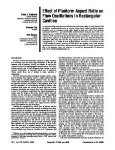
Figure 9. View of simulated potholes.
distance value is returned through an RS232 serial port to the central controller. The central controller uses this input to drive the motion control system. The range of this system is 40 ft. 3.4. Pothole Detection The robot also has the ability to detect and avoid simulated potholes represented by 2 ft diameter white circles randomly positioned along the course. A noncontact vision approach has been taken since simulated potholes are significantly different visually from the background surface. A monochrome Panasonic CCD camera is used to capture an image of the course ahead of the robot. The data from the camera is fed to the Epix™ imaging board. The control software for the imaging board processes the formatted data. This software makes extensive use of the XCOBJ/PXIPL image processing libraries provided by Epix™ to detect the presence of a simulated pothole and determine the location of the centroid of the pothole. The line following, obstacle avoidance and pothole detection systems are integrated for pothole detection and avoidance. The obstacle avoidance system takes precedence over the pothole avoidance system. Figure 9 shows view of simulated potholes that can be detected. 3.5. Navigational Challenge Problem and Solution The goal of the navigational challenge is to navigate Bearcat III to a series of predefined waypoints while avoiding obstacles. For this a global positioning system (GPS) is used to get the original robot position,
• embedded navigation features, • WAAS capability to improve accuracy of standard GPS signal to 3 m, • RS-232 serial port input/output to interface with robot’s computer, • external antenna for accurate reception, and • external power capability to ensure constant source of regulated power. Based on the above selection criteria the Garmin-76™ GPS was chosen as the unit to provide GPS navigational ability to the robot. The Garmin-76™ unit provides all of the above-mentioned features in addition to other features not used in the current navigation algorithm. 3.5.2. Description of Navigational Challenge Algorithm The basic solution selected to solve the navigational challenge problem was to model the problem as a basic closed feedback control loop. This model has an input command (target waypoint destination), feedback signal (GPS unit position information), error signal, and transfer function of the output characteristics. The GPS unit uses the current position information (latitude, longitude, height and velocity information at the rate of 1 to 255 second/output) and calculates the bearing and range from the target waypoint to determine the error. Correction signals are generated to reduce the error to a certain tolerance based on the bearing angle error signal generated by the GPS unit. The correction signals consist of turn right, turn left, forward motion, or stop. These corrective commands are sent to the motion control system, which translates these commands into motor control voltages that steer and propel the robot on the course. Once the bearing angle error and target range have been reduced to the required tolerance the
478
•
Journal of Robotic Systems—2004
Figure 10. Failure to detect short and overhung obstacles.
command is considered complete and the robot arrives at its target destination waypoint. At this point, the next target waypoint is selected and the process is repeated until all target waypoints in the database have been reached. The GPS signal is very poor inside buildings; however, the terrain is relatively flat and even. Here the data from the wheel encoders provide data for the motion control. This system is also used at the start until the velocity reaches a point that provides accurate GPS data. 3.5.3. Point to Point Navigation Using Wheel Encoders An encoder translates motion into electrical pulses, which are fed back into the Galil motion controller. The feedback is used to calculate the distance traversed. Steering is achieved by differential motion of the two wheels. The problem is modeled as a closed feedback control loop. The input command is the target waypoint destination relative to the robot position. The wheel encoder provides the feedback signal. The motion from the origin A to target B is achieved by two motions. The program calculates Angle ‘‘␣’’ and distance ‘‘d.’’ The robot first steers ‘‘␣’’ units and it then traverses ‘‘d’’ units to reach the target.
Figure 11. Failure to differentiate a ramp from a short obstacle.
detect the ramp or the ground as an obstacle, giving rise to misinterpretation of the environment. A simple case is illustrated in Figure 11 when the system detects the ramp as an obstacle. The algorithm fails to handle the case when the situation becomes dynamic. It will change its path to avoid all the obstacles it sees every time it scans the surrounding. It fails to take into account the trajectory of the moving obstacles. The alternate path taken by the robot may result in hitting the obstacle if both the robot and the obstacle move in the same direction. The algorithm also fails when the configuration of obstacles becomes so complex such that it will not have a way to go further. A simple case is illustrated in Figure 12. In such situations, there is always an option to retrace its path and look for a different path to avoid the deadlock. The algorithm does not have any kind of memory mapping, so the robot comes to a stop when it enters a deadlock. 3.7. Algorithm Implementation The physical implementation of the feedback control loop of the GPS navigation consists of the Garmin 76 GPS unit, the motion control system, laser scanner, and the robot computer. Waypoint coordinates are read from the waypoints file during the initialization stage of the program and stored in an array in
3.6. Obstacle Avoidance A single line Sick Optics™ laser scanner is used to detect and avoid obstacles. If an obstacle is detected, an obstacle avoidance routine, similar to the feedback control loop used for the GPS navigation, is used to navigate the robot around the obstacle. Once the robot avoids the obstacles, the original target waypoint is restored and the navigational feedback control loop is resumed. This approach has some limitations. The Bearcat has only one laser scanner. It scans a single plane at the mounted height, limiting it from detecting obstacles that are either short or overhung as shown in Figure 10. If the laser scanner is mounted at a shorter height, it will detect shorter obstacles, but this will lead to a different problem. When the terrain is not plane but wavy, or if there are ramps, the scanner will
Figure 12. Robot in a deadlock.
Ghaffari et al.: Unmanned Ground Vehicle, Bearcat III
memory. A NMEA message is sent to the Garmin 76 GPS unit via the RS 232 port, which sets the active target waypoint in the GPS unit’s memory. This is the command signal. Once set, the waypoint coordinate is used by the GPS unit to calculate bearing, track, and range to the target waypoint. The Garmin 76 GPS unit transmits ASCII data output via the RS232 port containing the bearing, track, and range to the destination waypoint. The turn angle (angle error) is related to the track angle and bearing angle by the equation: Turn Angle⫽Track Angle–Bearing Angle. This equation gives the turn angle in the 0 to 360 deg reference frame but this angle is transformed to 0 to 180 deg (left turn angle) or 0 to ⫺180 deg (right turn angle) for the robot turning subroutine. The robot turns to the commanded correction turn angle if the turn angle is greater than 6 deg or less than ⫺6 deg and then moves forward until the GPS position data are updated. When the robot arrives within 5 ft of the destination waypoint, the next target waypoint is selected and this process is repeated until all targets have been reached. This process defines the discrete feedback control loop algorithm used for the robot GPS navigation course.
•
479
Table I. Predicted performance. Task
Predicted performance
1
Line following
Tracks lines with an accuracy of 0.3 in.
2
Obstacle avoidance
Detects obstacles 8 in. and higher in a range of 24 ft
3
Pothole detection
Detects simulated potholes across the 10 ft track and a distance of 4 ft
4
Waypoint detection
Navigates way points with an accuracy of 6 ft
5
Emergency stop
Has a remote controlled emergency stop that can be activated from a distance of 65 ft
6
Dead end detection
Detects dead ends and avoids traps bybacking up and following alternative route
7
Turning radius
Vehicle has a zero turning radius
8
Maximum speed
5 mph
9
Ramp climbing ability Can climb inclines up to 10%
10
Braking distance
Vehicle comes to a dead stop as soon as the power is cut off
4. PREDICTED AND ACTUAL PERFORMANCE The predicted performance for the major tasks required of the contest is shown in Table I. Actual performance at the contest has varied depending on the software, weather and sometimes luck. We have learned to do a Potential Failure Modes and Effects Analysis (PFMEA) and a large amount of precontest testing. The most predictable failure is battery discharging so a digital voltmeter is used. Other events such as hard drive crashes led to shock mounted, dual drives. Loose connections can be quickly detected with a voltmeter. A rain cover is used in wet weather.
5. CONCLUSION Several aspects of the design and implementation of an unmanned ground vehicle were explained. A dynamic model was constructed and the robot parameters were computed to provide a basis for control and learning studies. The main sensory systems and algorithms for line following, waypoint navigation, and pothole detection were described. The design has been proved rugged and robust in the International Ground Vehicle Competition as well as many other
experiments. The UC robot team currently is using the lessons learned from Bearcat III to design a completely new robot called Bearcat Cub and is preparing to compete in the next IGVC with the new robot. Overall, this contest has been a wonderful educational experience and a great proving ground for ideas.
ACKNOWLEDGMENTS The authors would like to thank all the former and current UC robot team members, especially Shince Francis, Suresh Paul, Raymond Scott, Balaji Sethramasamyraja, Peter Cao, Pravin Chandak, Dinesh Dhamodarasamy, Maurice Tedder, Vikram Vaidyanathan, Sachin Modi, Steven Michalske, Sugan Narayanan, and many other students listed on www.robotics.uc.edu that have contributed their time and efforts to the design and construction of the robot and leadership of the team. Rob Hicks has served admirably as a dedicated industry advisor. We also gratefully acknowledge our organizational sponsors: Chapter 21 of the Society of
480
•
Journal of Robotic Systems—2004
Manufacturing Engineers, General Electric Aircraft Engines, Procter & Gamble, Kroger’s, ROV Technologies, FSR, Futuba, Timely Creations, K’s Structured Engineering, Freewave, EPIX Imaging, AFG, American Showa, Planet Products, UC Student Organizations and Activities, UC Graduate Student Association, Mr. Jim’s Steakhouse, the Department of Mechanical, Industrial and Nuclear Engineering, and the College of Engineering. We also gratefully acknowledge our individual sponsors: Dr. Eugene Merchant, Dr. Richard Shell, Dr. Ronald L. Huston, Dr. Richard L. Kegg, Mohan Kola, Ronald Tarvin, Merton D. Corwin, Richard E. Hohn, Jin Cao, Fred Reckelhoff, Dinesh Kumar Dhamodarasamy, Priya K. Das, Sameer Parasinis, Rob Hicks, Karthikeyan Kumaraguru, Aravind Muralidharan, Jin Cao, Vishnuvardhanaraj Selvaraj, Meyyapa Ganesh Murugappan, Jeyaprakash Thayalan, Robert F. Kostruck, Terrell L. Mundhenk, Dr. Rivett, Dino T. Vlahakis, Nikhil Kelkar, Larry Daprato, Tayib Samu, and Shaojian Deng. Finally, the technical staff of the University of Cincinnati has guided us through many difficult technical problems. We would especially like to thank Dave Breheim and Doug Hurd of the machine shop; Larry Schartman and Bo Westheider for their computer and network support; Dr. Frank Gerner, Sue Lyons and Luree Blythe in the MINE office for their great administrative support and Dean Stephen Kowel and Dean Roy Eckart for their encouragement and leadership.
REFERENCES 1. A.N. Goritov and A.M. Korikov, Optimality in robot design and control, Autom Remote Control 62 (2001), 1097–1103. 2. J.B. Pollack, G.S. Hornby, H. Lipson, and P. Funes, Computer creativity in the automatic design of robots, Leonardo 36 (2003), 115–121. 3. A. Elfes, S.S. Bueno, M. Bergerman, E.C. de Paiva, and J.G. Ramos, Robotic airships for exploration of planetary bodies with an atmosphere: Autonomy challenges, Autonom Robots 14 (2003), 147–164.
4. S. Hirose, H. Kuwahara, Y. Wakabayashi, and N. Yoshioka, The mobility design concepts/characteristics and ground testing of an offset-wheel rover vehicle, Space Technol 17 (1997), 183–193. 5. T. Ito and S.M. Mousavi Jahan Abadi, Agent-based material handling and inventory planning in warehouse, J Intell Manuf 13 (2002), 201–210. 6. M.D. Letherwood and D.D. Gunter, Ground vehicle modeling and simulation of military vehicles using high performance computing, Parallel Comput 27 (2001), 109–140. 7. M. Ghaffari, S. Narayanan, B. Sethuramasamyraja, and E. Hall, Internet-based control for the intelligent unmanned ground vehicle: Bearcat cub, presented at SPIE Intelligent Robots and Computer Vision XXI: Algorithms, Techniques, and Active Vision, Providence, RI, 2003. 8. B. Sethuramasamyraja, M. Ghaffari, and E. Hall, Automatic calibration and neural networks for robot guidance, presented at SPIE Intelligent Robots and Computer Vision XXI: Algorithms, Techniques, and Active Vision, Providence, RI, 2003. 9. X. Liao, M. Ghaffari, S.M.A. Ali, and E. Hall, Creative control for intelligent autonomous mobile robots, intelligent engineering systems through artificial neural networks, in Intelligent engineering systems through artificial neural networks, Vol. 13, ASME, New York, 2003, pp. 523–528. 10. M. Colenso and Europe Japan Center, Kaizen strategies for improving team performance: how to accelerate team development and enhance team productivity, Financial Times, Prentice Hall (Pearson Education), London, 2000. 11. W. Wu, H. Chen, and P. Woo, Time optimal path planning for a wheeled mobile robot, J Robot Syst 17 (2000), 585–591. 12. S.M. Alhaj Ali, Technologies for autonomous navigation in unstructured outdoor environments, University of Cincinnati, Cincinnati, OH, 2003. 13. S.M. Alhaj Ali, M. Ghaffari, X. Liao, and E. Hall, Dynamic simulation of computed-torque controllers for a wheeled mobile robot autonomous navigation in outdoor environments, in Intelligent engineering systems through artificial neural networks, Vol. 13, ASME, New York, 2003, pp. 511–516. 14. R. Rajagopalan, A generic kinematic formulation for wheeled mobile robots, J Robot Syst 14 (1997), 77–91. 15. J. Lobo, C. Queiroz, and J. Dias, World feature detection and mapping using stereovision and inertial sensors, Robot Autonom Syst 44 (2003), 69–81.