plant reaching a capacity of 100 t/a was designed containing app. 1,900 m2 of parabolic ... The investment and production costs were compared and graded.
eigenvalues for controller designs in Yang and Mote 1. The behavior of closed-loop eigenvalues for the companion problem of a controlled translating beam has ...
AV1-LAB was employed. The engine characteristics are cited in. Table 1. The engine was fueled ... SOCIETY OF MECHANICAL ENGINEERS for publication in the ASME JOURNAL OF. ENGINEERING ..... Ag. Eng., Moscow, ID, pp. 117â131.
aCab b where. T. U1 ,U2 ,U3 , . (1). For thin-walled beams this problem was first posed in Reissner and Tsai 1. However, the approach employed therein led to a.
G. Belforte, T. Raparelli, V. Viktorov, G. Eula, and A. Ivanov. 174 Instantaneous ...... 10 Slotine, J.-J. E., and Li, W., 1991, Applied Nonlinear Control, Prentice-Hall,.
to the austenitic pipework to ensure a good final junction Fig. 1. Superficial defects .... The plastic strain rate (Ëp) can be decomposed as the sum of three terms 5, ...
196 Robust Speed Control of a Variable-Displacement Hydraulic Motor Considering Saturation Nonlinearity ...... 9 Utkin, V. I., 1992, Sliding Modes in Control and Optimization, Springer- ...... There is no guarantee that there exists a pair P, such th
9,10 modeled cartilage as a network of elastic fibers embedded in an elastic gel and prestressed by the Donnan osmotic swelling pressure (D) of the PGs.
cracks. The method makes use of the transfer matrix and Fourier .... Transactions of the ASME ... ther converted to standard Cauchy singular integral equations. 1 .... 10 Neerhaff, F. L., 1979, ''Diffraction of Love Waves by a Stress-Free Crack of.
was used to study finite simple shear of simulated ligament material parallel to the fiber ... medial collateral ligament to inhomogeneous, large deformation.
structures has become a standard approach in the design process of a large number of ..... modal analysis module of the free INRIA software Scilab 23. The.
received by the Dynamic Systems and Control Division November 2, 1998. Associ- ...... 5 Lee, F. C., Flashner, H., and Safonov, M. G., 1995, ''Positivity-Based Control ...... 16 Larsson, P. T., 1999, Controller Design for Linear Systems Subject to Act
swept volume is developed using advanced sweeping/skinning techniques. Semi- ... Tradition- ally, machining verifications were performed by first examining ... mercial CAD/CAM software CATIA to determine the boundary of engaged surface ...
rameters, such as pressure, velocity, and density, as well as pro- ... downstream and impinge on the aft wall of the cavity, thereby ... only a few investigations involved in evaluating the frequency and ..... Lx*. 2 ny. Ly*. 2 nz. Lz*. 2 1/2. (1) wh
backs being the high number of moving parts that they comprise, for their functioning relies on a .... force that opposes this motion. The action of each of these ...
Case 3âAnnular Flow. The time responses for liquid super- .... tional Meeting on Multiphase Flow, Cannes, France, June 7â9, pp. 307â327. 4 Marti, S., Erdal, F., ...
Introduction. The most commonly used mathematical formulation for a beam with a constrained layer damping treatment was developed by. Mead and Markus 1.
Department of Mechanical Engineering and. Applied Mechanics, ..... tem used is a quarter car suspension system that includes a driver. ..... lished as a Report of the UM IVHS Program. 10 Rakheja, S. ... 17â20, SCS, San Diego, CA. 12 Stein ...
interface strength in the void growth and coalescence process. Cox and Low .... shear lip regions is highly localized in the form of shear deformed voided bands ...
flow notably alters the distribution of wall shear stress at the bed of the anastomosis, reducing the peak ... As a natural starting point, most of the numerical and in-vitro .... achieved by reducing the characteristic size of an element or in- crea
ASME,. M. M. Yovanovich. Professor Emeritus and Principal Scientific Advisor, ... Gray 1 and Kokkas 2 present steady-state and transient so- lutions, based on ...
e-mail: [email protected]. V. S. Deshpande. Engineering ... beams of the same mass via three-dimensional finite element FE simulations. In these FE ...
''how good is good enough?'' Some aspects of the repair outcome may be inferior, but other mechanical characteristics of the repairs and replacements might ...
tures earlier than expected from standard linear cosmological models of Weinberg ... Transactions of the ASME .... phase mixing or free streaming, Kolb and Turner 5 p. 351. ... larger than LH because the speed of information transfer is limited.
systems, the readers are referred to Rossikhin and Shitikova 1 and the ... MECHANICAL ENGINEERS for publication in the ASME JOURNAL OF APPLIED ...... 1 Evans, A. G., Ito, Y. M., and Rosenblatt, M., 1980, ''Impact Damage Thresh-.
Journal of Applied Mechanics
Brief Notes A Brief Note is a short paper that presents a specific solution of technical interest in mechanics but which does not necessarily contain new general methods or results. A Brief Note should not exceed 1500 words or equivalent 共a typical one-column figure or table is equivalent to 250 words; a one line equation to 30 words兲. Brief Notes will be subject to the usual review procedures prior to publication. After approval such Notes will be published as soon as possible. The Notes should be submitted to the Editor of the JOURNAL OF APPLIED MECHANICS. Discussions on the Brief Notes should be addressed to the Editorial Department, ASME International, Three Park Avenue, New York, NY 10016-5990, or to the Editor of the JOURNAL OF APPLIED MECHANICS. Discussions on Brief Notes appearing in this issue will be accepted until two months after publication. Readers who need more time to prepare a Discussion should request an extension of the deadline from the Editorial Department.
A New Lagrangian and a New Lagrange Equation of Motion for Fractionally Damped Systems O. P. Agrawal
2 A New Lagrangian and a New Lagrange Equation of Motion This section presents a new Lagrangian and a new Lagrange equation of motion for a fractionally damped system. There are several definitions of a fractional derivative. Here a fractional derivative is defined in the Riemann-Liouville sense 共关4兴兲:
Professor, Mechanical Engineering and Energy Processes, Southern Illinois University, Carbondale, IL 62901
D ␣x共 t 兲⫽
d d ␣x共 t 兲 1 ␣ ⫽ dt ⌫ 共 1⫺ ␣ 兲 dt
冕
t
0
x 共 t⫺u 兲 du, u␣
t⬎0, 0⬍ ␣ ⬍1.
1
Introduction
All dynamic systems exhibit some degree of internal damping. Recent investigations have shown that a fractional derivative model provides a better representation of the internal damping of a material than an ordinary derivative model does. For a survey of fractional damping models and their applications to engineering systems, the readers are referred to Rossikhin and Shitikova 关1兴 and the references therein. Traditionally, the Newton’s law is used to model such nonconservative systems, and when a Lagrangian, Hamiltonian, variational, or other energy-based approach is used, it is modified so that the resulting equations match those obtained using the Newtonian’s approach. Several attempts have been made to include nonconservative forces in the Lagrangian and the Hamiltonian mechanics. Riewe 关2,3兴 presented a succinct survey of research in this area. He also pointed out that a term proportional to d n x/dt n in the EulerLagrange equation follows from a Lagrangian with a term proportional to (d n/2x/dt n/2) 2 . Hence, a frictional force of the form c(dx/dt) may follow directly from a Lagrangian containing a term of the form (d 1/2x/dt 1/2) 2 . Using this as the starting point, he developed a new approach to mechanics that allows nonconservative terms 共both ordinary and fractional damping兲 to be included in Lagrangians and Hamiltonians. This paper presents another form of a Lagrangian and the Lagrange equation that can be used to obtain equations of motion of systems whose damping forces are proportional to a fractional derivative of order j/n. With a minor change in the formulation, the resulting equations can be thought of as a state space representation of Riewe’s formulation 共关2,3兴兲. Contributed by the Applied Mechanics Division of THE AMERICAN SOCIETY OF MECHANICAL ENGINEERS for publication in the ASME JOURNAL OF APPLIED MECHANICS. Manuscript received by the ASME Applied Mechanics Division, June 7, 1999; final revision, Apr. 24, 2000. Associate Editor: A. A. Ferri.
Journal of Applied Mechanics
(1)
This definition can be extended for ␣⬎1. Here x(t) represents a state space coordinate of the dynamical system. The Lagrangian and the Lagrange equation of motion are given as L⫽ 1 共 ␣ 兲 21 共 D ␣ y 兲 T M D ␣ y⫺ 21 y T Ky⫹Q T y,
(2)
and
⫺1 1 共␣兲
d␣ L L ⫺ ⫽0 dt ␣ 共 D ␣ y 兲 y
(3)
where y is a state vector, M and K are the mass-like and the stiffness-like matrices, 1 ( ␣ ) is a ␣-dependent coefficient, and Q is a vector of generalized forces. The purpose of 1 ( ␣ ) is to make the formulation consistent with the variational 共or EulerLagrange兲 approach 共关2,3兴兲. Since 1 ( ␣ ) does not appear in the equations of motion, it will not be included, and its expression will not be given here 共for its expression see 关2,3兴兲. The Lagrangian L defined in Eq. 共2兲 is applicable for positive rational ␣ only. The dimensions of y, M, and K depend on the denominator part of ␣. Therefore, in this setting, L cannot be developed for irrational ␣. Matrices M and K are not the traditional mass and stiffness matrices. It will be seen that M may contain the mass and the damping, and K may contain the mass, the damping, and the stiffness. In the case of zero damping, M and K reduce to the mass and the stiffness matrices. It is assumed that, for the functions considered here, the composition rule applies. Substituting Eq. 共2兲 into Eq. 共3兲, we get the equation of motion as M D 2 ␣ y⫹Ky⫽Q.
(4)
To generate L, we need ␣, y, M, K, and Q. ␣ is half of the lowest common fractional derivative order. Thus, for a force of the form (d j/n x/dt j/n ), ␣ ⫽1/(2n). ␣ can be smaller. However, the smaller ␣ introduces no new modeling capability. The elements of the
state vector y are defined as y i ⫽D 2 ␣ y i⫹1 ⫽D 1/n y i⫹1 , (i ⫽1, . . . ,l⫺1), and y l ⫽x(t), where l⫽2n is the dimension of the vector. Now consider that mD 2 x, cD j/n x, and kx represent the inertia, the damping, and the spring forces, where m, c, and k are, respectively, the mass, the damping coefficient, and the stiffness of the system. In this case, M and K are given as
M⫽
K⫽
冤
冋
¯
0 ]
¯
0 ]
0 ]
¯
m
¯
c
¯
¯
c
]
¯
0
册
0 0
⫺c
0
]
⫺c
0
0
0
0
¯
0
⫺m
0
0
⫺m
0
0
0
0
⫺m
0
⫺c
0
0
⫺m
0
⫺c
0
0
⫺m
0
⫺c
0
0
0
0
k
0
0
0
0
共 D y 兲 M 2D 1/6
T
1/6
y⫺ 21
T
冥
,
y K 2 y,
d 1/6 L L ⫽0. ⫺ dt 1/6 共 D 1/6y 兲 y
⫺m
⫺m
0
0
,
0
0
]
冤
0
0
L⫽ 21
m
] ¯
]
]
m
¯
0
K 2⫽
0
0
0
k
冥
.
(5)
In matrix M the off-diagonal contains m and the jth off-diagonal measured from the bottom right corner contains c. In matrix K the bottom right corner contains k, the elements left to the offdiagonal contain ⫺m, and all except the first and the last elements of the ( j⫹1)th off-diagonal measured from the bottom right corner contains ⫺c. Note that M and K are symmetric. Structure of these matrices will be explained further using two examples. Finally, vector Q is given as Q⫽ 关 0,¯,0,F 兴
(6)
These terms give M 2 D 1/3y⫹K 2 y⫽0, which is equivalent to mx¨ ⫹cD 4/3x⫹kx⫽0. Note that M may contain m and c, and K may contain m, c, and k. Also, note that in the examples c can be set to zero to obtain the differential equations of motion of an undamped system in a higher dimension. Similarly, ␣ in Example 1 can be set to 1/4 to obtain the differential equations of motion of a damped system in a higher dimension. However, such increase in dimensions adds no benefit. Further, as the order of the fractional derivative ␣ moves from 1 towards 0 共1 towards 2兲 the damper behaves like a spring 共mass兲. Several techniques have been developed to solve the resulting set of fractional differential equations. Suarez and Shokooh 关5兴 presented an eigenvector expansion method to solve these differential equations. Other methods to solve these fractional differential equations include, for example, Laplace transform and direct techniques similar to the techniques for ordinary differential equations 共关6–8兴兲, and the numerical techniques 共关9兴兲.
3
Additional Remarks
where F is the generalized force. The Lagrangians and the Lagrange equations of motion for two fractionally damped systems are given below. Example 1. Damping force ⫽ cx˙ . For this system, ␣⫽1/2. Vector y, matrices M ⫽M 1 and K ⫽K 1 , the Lagrangian L, and the Lagrange equation are
Riewe 关2,3兴 developed a new approach to mechanics with fractional derivatives that includes the nonconservative Hamiltonian, Canonical transformations and the Jacobi theory. The approach can also be used to develop similar Hamiltonians and the Hamilton equations. To this end, we propose the following Hamiltonian and Hamilton equations for fractional systems.
y⫽ 关 y 1 y 2 兴 T ⫽ 关 x˙ x 兴 T ,
H⫽ 共 D ␣ y 兲 T p⫺L⫽ 共 D ␣ y 兲 T p⫺ 21 共 D ␣ y 兲 T M D ␣ y⫹ 21 y T Ky,
M 1⫽
冋 册 0
m
m
c
K 1⫽
,
冋
⫺m
0
0
k
册
L⫽ 21 共 D 1/2y 兲 T M 1 D 1/2y⫺ 21 y T K 1 y, d 1/2 L L ⫽0. ⫺ dt 1/2 共 D 1/2y 兲 y
y⫽ 关 y 1 y 2 y 3 y 4 y 5 y 6 兴 T
0
0
0
0
0
m
0
0
0
0
m
0
0
0
0
m
0
c
0
0
m
0
c
0
0
m
0
c
0
0
m
0
c
0
0
0
340 Õ Vol. 68, MARCH 2001
H ⫽⫺D ␣ p, y
where p⫽M D ␣ y. It can be shown that the above equations lead to the correct equation of motion. Using these equations, the Hamiltonian can also be written as
which is similar to the total energy term for a conservative system.
Acknowledgment The author would like to thank the reviewers for their suggestions to improve the quality of the paper.
References
⫽ 关 D 5/3x D 4/3x D 1 x D 2/3x D 1/3x x 兴 T ,
冤
and
H⫽ 21 共 D ␣ p 兲 T M ⫺1 D ␣ p⫹ 21 y T Ky,
These terms give M 1 Dy⫹K 1 y⫽0, which is equivalent to mx¨ ⫹cx˙ ⫹kx⫽0. Example 2. Damping force⫽cD 4/3x. This example shows the locations of c when j in the force term cD j/n x is more than 1. For this system, ␣⫽1/6. Vector y, matrices M ⫽M 2 and K⫽K 2 , the Lagrangian L, and the Lagrange equation are
M 2⫽
H ⫽D ␣ y, p
,
冥
,
关1兴 Rossikhin, Y. A., and Shitikova, M. V., 1997, ‘‘Applications of Fractional Calculus to Dynamic Problems of Linear and Nonlinear Hereditary Mechanics of Solids,’’ Appl. Mech. Rev., 50, No. 1, pp. 15–67. 关2兴 Riewe, F., 1996, ‘‘Nonconservative Lagrangian and Hamiltonian Mechanics,’’ Phys. Rev. E, 53, No. 2, pp. 1890–1899. 关3兴 Riewe, F., 1997, ‘‘Mechanics With Fractional Derivative,’’ Phys. Rev. E, 55, No. 3, pp. 3581–3592. 关4兴 Oldham, K. B., and Spanier, J., 1974, The Fractional Calculus, Academic Press, New York. 关5兴 Suarez, L. E., and Shokooh, A., 1997, ‘‘An Eigenvector Expansion Method for the Solution of Motion Containing Fractional Derivatives,’’ ASME J. Appl. Mech., 64, pp. 629–635. 关6兴 Miller, K. S., and Ross, B., 1993, An Introduction to the Fractional Calculus
Transactions of the ASME
and Fractional Differential Equations, John Wiley and Sons, New York. 关7兴 Mainardi, F., 1997, ‘‘Fractional Calculus: Some Basic Problems in Continuum and Statistical Mechanics,’’ Fractals and Fractional Calculus in Continuum Mechanics, A. Carpinteri and F. Mainardi, eds., Springer-Verlag, New York, pp. 291–348. 关8兴 Podlubny, I., 1999, Fractional Differential Equations, Academic Press, New York. 关9兴 Yuan, L., and Agrawal, O. P., 1998, ‘‘A Numerical Scheme for Dynamical Systems Containing Fractional Derivatives, Proceedings of the DETC98, ASME Design Engineering Technical Conferences, Paper No. DETC98/ MECH 5857, Sept. 13–16, Atlanta, GA.
On the Unification of Yield Criteria S. C. Fan Associate Professor, School of Civil & Structural Engineering, Nanyang Technological University, Nanyang Avenue, Singapore 639798
M.-H. Yu Professor, School of Civil Engineering & Mechanics, Xi’an Jiaotong University, Xi’an 710049, China
S.-Y. Yang Post Doctoral Fellow, School of Civil & Structural Engineering, Nanyang Technological University, Nanyang Avenue, Singapore 639798
A piecewise linear unified yield criterion called the twin-shearunified was proposed. It is based on a kind of orthogonal dodecahedron stress element. The effects of intermediate principal stress are taken into account such that most available yield loci on the -plane are embraced in a unified manner. Besides, it is capable to represent not only convex limit surfaces but also nonconvex limit surfaces. 关DOI: 10.1115/1.1320451兴
1
Introduction
line 1 ⫽ 2 ⫽ 3 in the principal stress space兲. Many derivatives of these two criteria have been proposed to model a wider range of engineering materials. Among them, the well-known ones are Mohr-Coulomb, Hoek-Brown, and Johnson 共Tresca’s derivatives兲, Matsuoka and Lade 共Mises’ derivatives兲 关1兴. The Mohr-Coulomb is a max⫺ criterion which considers the effect of max as well as the normal stress on the same plane. The introduction of makes it capable of simulating materials with different tensile and compressive strengths t ⫽ c 共called the strength differential effect or SD effect兲. The Hoek-Brown and Johnson are MohrCoulomb’s derivatives for rock. They take into account the effect of nonlinear failure loci on the meridian plane while the MohrCoulomb does not. The Matsuoka and Lade are failure theories for soil 共sand兲. They account for both the SD effect and the nonlinear failure loci on the meridian plane. Unfortunately, recent research revealed that those theories do not necessarily represent the real failure/yield of materials under complex stress state. One prominent feature has been ignored, i.e., the effect of the intermediate principal stress ( 2 ). The Tresca and its derivatives ignore this effect whereas the Mises and its derivatives average the effects of all the three principal stresses 1 , 2 , 3 . Experiments show that the 2 effect varies from case to case 共关2–5兴兲. The extent of the 2 effect depends on the material type and the stress state. The second category of yield criteria may be called curvefitting multiparameter criteria such as the Argyris-GudehusZienkiewicz criterion, the Willam-Warnke criterion, and some smooth models 共关1兴兲. These criteria usually have complex mathematical expressions because simple expressions usually cannot reflect the diversity of test results. The main advantage is that they can simulate accurately the yield properties in the particular range of complex stress state where most tests are conducted. Another deficiency is that they have little physical background.
2.1 The TS-Unified Criterion Bridges Most Available Theories on Plane. The TS-unified is an extension of the twin shear yield criterion 共TS兲 共关6兴兲 and the generalized twin shear yield criterion 共GTS兲 共关7兴兲. The TS is based on a kind of orthogonal dodecahedron 共OD兲 stress element and it assumes that when a function of the two larger principal shear stresses ( 13 , 12) or ( 13 , 23) reaches a critical value, the material begins to yield, i.e.,
For many engineering materials, two characteristic strength properties are crucial, i.e., initial and subsequent yield properties. The initial yield defines the critical state when the material under the complex stress state starts to yield. The subsequent yield deals with the post yield phenomena. It describes the material behavior beyond the initial yield. The initial yield provides the basis. As long as the initial yield property is defined, the remaining task is to define the different hardening/softening properties and to incorporate them into the initial yield provided. In this note, the yield criteria will be confined to the initial yield properties unless otherwise stated. Generally speaking, yield criteria can be classified into two categories. The first category has originated from the concept of a single shear stress yield criterion such as the Tresca and the Mises. The Tresca is a maximum principal shear stress max criterion. The Mises is an octahedral shear stress oct criterion. They both postulate that when max 共or oct兲 reaches a critical value, the material begins to yield. Both the Tresca and the Mises are applicable only to materials with 共i兲 equal tensile and compressive strengths t ⫽ c ; 共ii兲 linear failure loci on the meridian plane 共i.e., parallel to the hydrostatic axis which is represented by the Contributed by the Applied Mechanics Division of THE AMERICAN SOCIETY OF MECHANICAL ENGINEERS for publication in the ASME JOURNAL OF APPLIED MECHANICS. Manuscript received and accepted by the ASME Applied Mechanics Division, Feb. 16, 1999; final revision, Nov. 1, 2000. Associate Editor: M.-J. Pindera.
Journal of Applied Mechanics
13⫹ 12⫽ t
when 12⭓ 23
13⫹ 23⫽ t
when 12⭐ 23
(1)
Fig. 1 Different yield loci on the -plane for non-SD materials „ t Ä c or  Ä0…
⫽0, the GTS is simplified to the TS. So the TS is a special case of the GTS. In the TS and GTS, the largest stresses 共both the shear and the normal stresses兲 have the same extent of influence as that of the second largest. When different weight parameters are employed to reflect the different effects of the largest stresses and the second largest, the GTS can be generalized to the TS-unified. The TSunified can be expressed as 13⫹b 12⫹  共 13⫹b 12兲 ⫽C
when 12⫹  12⭓ 23⫹  23
13⫹b 23⫹  共 13⫹b 23兲 ⫽C
when 12⫹  12⭐ 23⫹  23
(3)
where b is a material parameter which represents the effect of the intermediate 共the second largest兲 principal stresses. The value of b can be determined by material tests.  and C are also material parameters. If uniaxial tensile and compressive strength 共 t and c 兲 are chosen as the basic test points, then  and C can be expressed as
⫽ Fig. 2 Different yield loci on the -plane for SD materials „ t Å c or Å0…
where 13⫽( 1 ⫺ 3 )/2, 23⫽( 2 ⫺ 3 )/2, 12⫽( 1 ⫺ 2 )/2 are the principal shear stresses. 1 , 2 and 3 ( 1 ⭓ 2 ⭓ 3 ) are the principal normal stresses. t is the uniaxial tensile strength. The TS is an upper limit surface in the stress space complying with Drucker’s convexity postulate and is used for non-SD materials 共 t ⫽ c , where c is the uniaxial compressive strength兲 only. It is the counterpart to the Tresca, as shown in Fig. 1. The GTS extends the idea and assumes that the yield surface is a function of two larger principal shear stresses ( 13 , 12) or ( 13 , 23) and their corresponding normal stresses ( 13 , 12) or ( 13 , 23), i.e., 2 t c when 12⫹  12⭓ 23⫹  23 c⫹ t (2) 2 t c 13⫹ 23⫹  共 13⫹ 23兲 ⫽ when 12⫹  12⭐ 23⫹  23 . c⫹ t
13⫹ 12⫹  共 13⫹ 12兲 ⫽
where 13⫽( 1 ⫹ 3 )/2, 12⫽( 1 ⫹ 2 )/2, 23⫽( 2 ⫹ 3 )/2. The parameter  reflects the effects of the normal stresses so that SD effect can be represented. Likewise, the GTS serves as the counterpart to the Mohr-Coulomb, as shown in Fig. 2. When
c ⫺ t 1⫺ ␣ ⫽ c ⫹ t 1⫹ ␣
C⫽
共 1⫹b 兲 t c 1⫹b ⫽ . c⫹ t 1⫹ ␣ t
(4)
where ␣ ⫽ t / c is the ratio of the tensile to the compressive strengths. The ratio is an index of the material strength differential effect 共SD effect兲. The TS-unified is a series of piecewise linear yield criteria on the -plane as shown in Figs. 1 and 2. The exact form of expression depends on the choice of parameter b, which in turn can be determined by some basic test results as illustrated in Section 2.3 of this note. The TS-unified has the following characteristics as shown in Table 1: 共a兲 With different choices of parameter b, the TS-unified can be simplified to the Tresca 共⫽0 and b⫽0兲, the linear approximations of Mises 共⫽0 and b⫽1/2 or ⫽0 and b⫽1/(1⫹))兲, the Mohr-Coulomb 共⫽0 and b⫽0兲, the TS 共⫽0 and b⫽1兲, the GTS 共⫽0 and b⫽1兲 and a series of new strength criteria 共other values of parameters  and b兲. 共b兲 In the stress space, the lower and upper bounds for the yield surfaces on the -plane are special cases of the TS-unified, i.e., b⫽0 共⫽0 for the Tresca or ⫽0 for the Mohr-Coulomb兲 and b⫽1 共⫽0 for the TS or ⫽0 for the GTS兲, respectively. 共c兲 When the parameter b varies between 0 and 1, a series of yield surfaces between the two limiting surfaces can be obtained. 共d兲 When the parameter b varies beyond the range 共i.e., b⬍0 or b⬎1兲, a series of nonconvex limit surfaces could be derived. 2.2 The TS-Unified Reflects Different 2 Effects. The Lode angle is a parameter to represent the relative value of 2
Table 1 The characteristics of TS-unified
b⫽0 plane loci Restriction for application 0⬍b⬍1 plane loci Restriction for applications b⫽1 plane loci Restriction for applications
342 Õ Vol. 68, MARCH 2001
⫽0 ( t ⫽ c ⫽ 0 )
⫽0 ( t ⫽ c )
Drucker’s Convex Postulate
Tresca Regular hexagon 0 0⫽ 2
Mohr-Coulomb Irregular hexagon tc 0⫽ c⫹t
Lower bound
New theories Irregular dodecagon 共b⫹1兲 0⫽ 共2⫹b兲 0
New theories Irregular dodecagon 共b⫹1兲tc 0⫽ t⫹共b⫹1兲c
Intermediate
Twin shear theory Regular hexagon 2 0⫽ 0 3
Twin shear theory Irregular hexagon 2tc 0⫽ t⫹2c
Upper bound
Transactions of the ASME
It should be noted that the stress angle is different from the Lode angle , and they are related as follows:
⫽ ⫺ . 6
(8)
Equation 共5兲 is the explicit expression for the TS-unified in terms of the stress angle . With different choices of the parameter b, the TS-unified can reflect different piecewise linear 2 effects. Two illustrations are given. Figure 3共a兲 shows the curves of 1 / t versus 2 / t for ␣ ⫽1 and 3 / t ⫽0.2. Obvious strength difference can be observed when different criteria are adopted 共represented by different values of the parameter b兲. The maximum difference is about 25 percent. Figure 3共b兲 shows the curves for ␣⫽1 and b⫽1. The same conclusion can be drawn as from Fig. 3共a兲. In other words, the TS-unified is capable of representing variable strengths of the same material under different stress states. 2.3 Application of the TS-Unified. If t , c and the shear strength 0 are chosen as the basic material parameters, through Eq. 共3兲 for pure shear loading, the parameter b can be expressed as b⫽
Fig. 3 TS-unified can reflect the 2 effect in a piecewise linear manner; „a… ␣Ä1 and 3 Õ t Ä0.2 case; „b… ␣Ä1 and bÄ1 case
where b is the stress angle when the two Eqs. 共5兲 are equal:
b ⫽tg⫺1
) , 1⫹2 ␣
共 0 deg⬍ b ⬍60 deg兲 .
(6)
The stress angle is defined to reflect the 2 effect as shown in Fig. 2, such that 1 3) J 3 ⫽ cos⫺1 3 2 冑J 32 Journal of Applied Mechanics
共 0⭐ ⭐ /3兲 .
(7)
(9)
The parameter b plays an important role in the TS-unified. It builds a bridge among different strength theories. It is this parameter that distinguishes one theory from another. On the other hand, the scope of application of each theory is also represented by this parameter. Hence, the TS-unified is a unified theory that can be applied to more than one kind of material. In practice, when basic material parameters are obtained by experiments, the value of b can be determined through Eq. 共9兲. Whenever parameter b is obtained, the yield criterion is determined and the application is possible 共关8兴兲.
3 with respect to 1 and 3 . To reflect the 2 effect, a theory should embed this parameter in its expression either in explicit or in implicit forms. The TS-unified is usually expressed in terms of the stress 共deviatoric兲 invariants, that is the first invariant of stress tensor I 1 , the second invariant of stress deviatoric tensor J 2 , and the stress angle , as follows:
共 c⫹ t 兲 0⫺ t c . 共 t⫺ 0 兲 c
Conclusions
A piecewise linear unified yield criterion called the TS-unified was proposed. Besides the capability that the TS-unified can bridge most available yield loci on the -plane for both SD and non-SD materials, the most prominent characteristics of the criterion are their capability to represent the effects of the intermediate principal stress 2 in piecewise linear forms. Illustrations were given. The determination of the parameters was also discussed. Future research could focus on the pursuit for some criteria that can bridge different criteria both on the -plane and on the meridian plane. It is obvious that the representation for nonlinear meridian loci can be obtained by adopting multiparameter criterion instead of the proposed two-parameter TS-unified.
References 关1兴 Chen, W. F., and Han, D. J., 1988, Plasticity for Structural Engineers, Springer-Verlag, New York. 关2兴 Mogi, K., 1967, ‘‘Effect of Intermediate Principal Stress on Rock Failure,’’ J. Geophys. Res., 72, pp. 5117–5131. 关3兴 Michelis, P., 1987, ‘‘True Triaxial Cyclic Behavior of Concrete and Rock in Compression,’’ Int. J. Plast., 3, No. 2, pp. 249–270. 关4兴 Faruque, M. O., and Chang, C. J., 1990, ‘‘A Constitutive Model for Pressure Sensitive Materials With Particular Reference to Plain Concrete,’’ Int. J. Plast., 6, No. 1, pp. 29–43. 关5兴 Li, X. C., and Xu, D. J., 1990, ‘‘Experimental Verification of Twin Shear Strength Theory—The Strength Properties of Granite Under True Triaxial Stress State,’’ Wuhan Institute of Rock and Soil Mechanics, Chinese Academy of Science, Paper Yantu 共90兲 52 共in Chinese兲. 关6兴 Yu, M. H., 1983, ‘‘Twin Shear Stress Yield Criterion,’’ Int. J. Mech. Sci., 25, No. 1, pp. 71–74. 关7兴 Yu, M. H., He, L. N., and Song, L. Y., 1985, ‘‘Twin Shear Stress Theory and Its Generalization,’’ Sci. Sinica A, 28, No. 1, pp. 1174–1183. 关8兴 Yu, M. H., Yang, S.-Y., and Fan, S. C., 1999, ‘‘Unified Elasto-Plastic Associated and Non-Associated Constitutive Model,’’ Comput. Struct., 71, No. 6, pp. 627–636.
MARCH 2001, Vol. 68 Õ 343
Analytical Solution for W-N Criteria for the Prediction of Notched Strength of an Orthotropic Shell R. Ramesh Kumar Engineer, Structural Design and Analysis Division, Structural Engineering Group, Vikram Sarabhai Space Centre, Thiruvananthapuram 695 022, India
S. Jose Senior Lecturer, Department of Mechanical Engineering, T.K.M. College of Engineering, Kollam 691 005, India
G. Venkateswara Rao Group Director, Structural Design and Analysis Division, Structural Engineering Group, Vikram Sarabhai Space Centre, Thiruvananthapuram 695 022, India
understanding of the maximum stress location is very essential. Unlike in metallic structures, for fiber-reinforced orthotropic shells, the maximum stress does not occur at the hole edge in a plane normal to the loading direction, but depends on the fiber orientations 共关5兴兲. Moreover, establishing convergence for the finite element model for the isotropic medium for a known problem does not ensure convergence for the orthotropic medium. Hence an analytical solution that can bring out the overall behavior of the orthotropic structure is very much required. Savin 关6兴 in his complex variable approach to the problem of stresses in an isotropic circular cylindrical shell with holes showed that the stress state in a shell is a sum of a plate solution and a function of curvature effect. Konish and Whitney’s 关5兴 and Kumar, Rao, and Mathew’s 关7兴 orthotropic equations 共plate兲 were based on the sum of an isotropic plate solution and a function of higher order term of distance ahead of the hole in terms of orthotropic material constants. Thus one can conjecture that the orthotropic shell solution in a polar coordinate system 共,兲 can be obtained as a sum of an isotropic plate equation 共first term in 共1兲兲, higher order term of distance ahead of a hole 共third term in 共1兲兲, and functions of isotropic and orthotropic curvature effects 共second and fourth terms in 共1兲兲.
Sh 共,兲
Analytical solution for the tangential stress distribution ahead of a hole is needed for the theoretical prediction of notched strength of brittle laminate using the well-known W-N criteria. In the present study, tangential stress distribution in an orthotropic circular cylindrical shell under uniaxial loading with a circular hole is obtained intuitively with the use of a stress function. A good agreement is obtained for the stresses around and ahead of the circular hole in 共 0 deg 4 ⫾ 30 deg 兲 s and 90 deg laminates with the finite element results. 关DOI: 10.1115/1.1320452兴
Introduction Prediction of failure strength of brittle laminate with a hole was very well established based on the W-N fracture criteria 共关1–4兴兲. Failure of the laminate occurs when the dominant stress near the hole or the average of the dominant stress over a region near the hole reaches the strength of the laminate. Konish and Whitney 关5兴 developed an analytical solution for the stress distribution near a hole in an orthotropic plate. For the shell-type composite structures one has to essentially go for the finite element approach as there is no such analytical solution available in the literature for employing the W-N criteria. For the best numerical results a clear
冋 冉 冊冉 冉 冊
冦冦
2A 共0j 兲
Im共 j 兲 ⫽
1
ln
2B 共0j 兲
⫹2
⫹
冋
␥ &
⫹
A 共2j 兲 ⫹
B 共2j 兲
2
⫽ Ortho
⫹f
冉 冉
⫹ f 共  兲 ISO ISO
higher order terms in with orthotropic coefficients higher order terms in with orthotropic coefficients for 
冊 冊
(1)
In the present work an analytical solution for the tangential stress distribution ahead of a circular hole in an orthotropic circular cylindrical shell under axial loading is obtained for use via the W-N criteria.
Analytical Solution for the Tangential Stress Distribution The most general solution for the stress distribution near cutouts of any arbitrary shape under tension or internal pressures up to an accuracy of  2 was given by Pirogov 关8兴. The equation with unknown coefficients 共like A 0 , B 0 , E K , F K , etc.兲 is of the form
F 共2j 兲 ⫺ 共 j兲 共 A 0 ⫹A 共2j 兲 兲 2 ⫹E 共2j 兲 ⫹ 2 cos 2 . 4
Contributed by the Applied Mechanics Division of THE AMERICAN SOCIETY OF MECHANICAL ENGINEERS for publication in the ASME JOURNAL OF APPLIED MECHANICS. Manuscript received by the ASME Applied Mechanics Division, May 4, 1999; final revision, May 25, 2000. Associate Editor: J. W. Ju.
冏
Pl共 , 兲 ⫹f
␥
Based on the above stress function, Savin obtained the tangential stress distribution around a circular hole of radius ‘‘a’’ in an
344 Õ Vol. 68, MARCH 2001
冏
冊
k⫺2 共 j 兲 B 共kj 兲 A ⫹ k cos k 2 k⫺2 k
冉
E 共kj 兲
k⫺2
⫹
F 共kj 兲
k
冊
cos k
冧
冧
(2)
isotropic shell of radius ‘‘R’’ and thickness ‘‘t,’’ under axial loading, as a sum of an isotropic plate solution ( Pl ( , )/ ) and a function of isotropic curvature parameter, . The solution is valid for a hole whose projected size 共on a plane passing through the axis of shell and normal to the axis of hole兲 is close to the actual hole size.
where  Ortho⫽ 关 冑3(1⫺ 2 )(E /E Y )/2兴 a/ 冑Rt, ⫽Poisson’s ratio, E and E Y are the moduli of elasticity in and Y 共loading direction兲 directions 共关9兴兲, and ( Pl ( , )/ ) for the orthotropic plate is available in Kumar et al. 关7兴. 4
Pl 共,兲
冏
⫽ Ortho
1⫺Cos 2 3 1 ⫹ 2 ⫺ 4 Cos 2 2 2 2 ⬁
⫹
兺
j⫽2
冋
册
⫺C 2 j 4 j⫺3 4 j⫺1 ⫺ 4 j Cos 2 j 2 4 j⫺2
(5)
Details of the orthotropic coefficients C 2 j 共 j varying from 1 to ⬁兲 are given in the Appendix. It can be noticed from Pirogov’s stress function given in 共1兲 that the higher order terms for the plate solution and  are of similar trigonometric relationship. Therefore, the functions of  may be expressed as
再冉 冊
2 1 3 f 共  兲 Ortho⫽⫺ 1⫹ 4 Cos 2 2 4
冋
⬁
⫹
册
冎
C 2 j 4 j⫺3 4 j⫺1 ⫺ 4 j Cos 2 j . 2 4 j⫺2
兺
j⫽2
(6)
Thus the final expression for the tangential stress distribution for an orthotropic circular cylindrical shell with a circular hole is given by
then one fourth up to ⫽2 in the radial direction, while in direction, it is at every five-degree interval along the circumference of the hole from 0 deg to 180 deg. Boundary Conditions. Symmetric boundary conditions are applied at the symmetric planes. Loading. A distributed load of 240 N is applied on the nodes at the top circumference. The load is distributed in each element in the ratio of 1:4:1 among the nodes in an element.
再冉 冊 冎 冉 冊 冎 冎 再兺 再
⫻
1⫹
⬁
⫻
Fig. 1 Tangential stress distribution around a circular hole in an orthotropic shell
In this work, circular cylindrical shells with (0 4 ,⫾30) S and (90) 12 lay ups made of high modulus M55J/M18 carbon/epoxy laminate having material properties E X ⫽328.949 GPa, E Y ⫽5.955 GPa, G XY ⫽4.414 GPa and XY ⫽0.346, with layer thickness of 0.1 mm is considered.
Finite Element Modeling The laminated circular cylindrical shell 共R⫽48 mm, t ⫽1.2 mm and height⫽180 mm兲 with a hole of radius a⫽5 mm is modeled using eight-noded layered shell elements available in NISA2 finite element software. Due to the symmetry, one fourth of the shell 共at its half height兲 is modeled. The region around the hole is modeled with a finer mesh with an element size of one tenth of the hole radius up to ⫽0.5, then one fifth up to ⫽1 and Journal of Applied Mechanics
Fig. 2 Tangential stress distribution ahead of a circular hole in an orthotropic shell
MARCH 2001, Vol. 68 Õ 345
Results and Discussion Initially, convergence of 共7兲 is established by progressively increasing the number of terms till a converged value is obtained. For the present cases terms up to C 22 ( j⫽11) are needed to achieve convergence within one percent. It may be noted that for  ⫽0, 共7兲 reduces to the orthotropic plate solution. Using 共7兲, the tangential stress distribution around a hole ( ⫽1) is obtained and compared with the finite element results as shown in Fig. 1. The maximum stress concentration factor of ⫺8.56 is observed at ⫽0 for (90) 12 laminate, as against the finite element result of ⫺8.71. The deviation in the results is estimated as two percent. In the case of (0 4 ,⫾30) S lay up, the peek stress occurs at ⫽90 deg as expected, with a stress concentration factor value equal to 5.18 as against the finite element result of 5.44. It can be noticed that the deviation between the two values is about five percent. The stress distributions away from the hole for ⫽1 to 2, for the two types of lay-up sequence considered are shown in Fig. 2. From the finite element analysis, it is found that as a percentage of total stress, bending stress constitute within two percent for the types of lay-up sequences considered. It is concluded that the present solution shows a reasonably good agreement with the finite element results.
Stress Wave Propagation in a Coated Elastic Half-Space due to Water Drop Impact Hyun-Sil Kim1 e-mail: [email protected]
Jae-Seung Kim Mem. ASME
Hyun-Ju Kang
Conclusion A new analytical solution for tangential stress distribution for an orthotropic circular cylindrical shell with a circular hole under axial loading is derived which gives good agreement with finite element results. The solution can be used with W-N criteria for the prediction of notched strength of an orthotropic shell with a circular hole.
Appendix There is a standard technique 共关10兴兲 for determining the Fourier coefficients C 2 j of a function as in 共7兲: A 0 C 0 ⫹A 2 C 2 ⫹A 4 C 4 ⫽2a 0
(A1a)
A 2 C 0 ⫹ 共 A 4 ⫹2A 0 ⫹ 兲 C 2 ⫹A 2 C 4 ⫹A 4 C 6 ⫽2a 2
(A1b)
and for j⬎3 a recursive relationship exists in the form C2 j⫽
关6兴 Savin, G. N., 1970, ‘‘Stress Distribution Around Holes,’’ NASA Technical Translation, NASA TTF-607. 关7兴 Kumar, R. R., Rao, G. V., and Mathew, K. J., 1999, ‘‘A New Solution for Prediction of Notched Strength for Highly Orthotropic Plate,’’ J. Aeronaut. Soc. India, 51, No. 1, pp. 28–34. 关8兴 Pirogov, I. M., 1962, ‘‘On Approximate Solution of Basic Differential Equations in the Theory of Shells,’’ Izv. Vuzov. Mash, 11. 关9兴 Lekhnitskii, S. G., 1947, Anisotropic Plates, Gordon and Breach, New York. 关10兴 Krylov, V. I., and Kruglikova, L. G., 1969, Handbook of Numerical Harmonic Analysis, Israel Program for Scientific Translations, Jerusalem.
⫺1 关 A 2 C 2 j⫺2 ⫹2A 0 C 2 j⫺4 ⫹A 2 C 2 j⫺6 ⫹A 4 C 2 j⫺8 兴 A4 (A1c)
where a 0 ⫽4k(n⫹k⫺1); a 2 ⫽⫺4k(n⫹k⫹1); A 0 ⫽3⫹n 2 ⫺2k ⫹3k 2 A 2 ⫽4 共 1⫺k 2 兲 ; n⫽N/K,
A 4 ⫽ 共 1⫺n 2 ⫹2k⫹k 2 兲
(A2)
¯ X /G ¯ XY N⫽ 冑2 共 K⫺¯ XY 兲 ⫺E
k⫽1/K,
¯Y K⫽ 冑¯E X /E
¯E X ,E ¯ Y ,¯ XY ,G ¯ XY are the overall orthotropic properties of the shell.
References 关1兴 Whitney, J. M., and Nuismer, R. J., 1974, ‘‘Stress Fracture Criteria for Laminated Composites Containing Stress Concentrations,’’ J. Compos. Mater., 8, pp. 253–265. 关2兴 Rhodes, M. D., Mikulas, M. M., and Mcgowen, P. E., 1984, ‘‘Effect of Orthotropy and Width on Compression Strength of Graphite-Epoxy Panels With Holes,’’ AIAA J., 22, pp. 1283–1292. 关3兴 Awerbuch, J., and Madhukar, M. S., 1985, ‘‘Notched Strength of Composite Laminates: Prediction and Experiments—A Review,’’ J. Reinf. Plast. Compos., 4, pp. 3–159. 关4兴 Kumar, R. R., 1993, ‘‘Experimental Investigation and Prediction on Notched Strength of Laminated Composite Circular Cylindrical Shells,’’ DLR report IB 131-93/16, Germany. 关5兴 Konish, H. J., and Whitney, J. M., 1975, ‘‘Approximate Stresses in an Orthotropic Plate Containing a Circular Hole,’’ J. Compos. Mater., 9, pp. 157–166.
346 Õ Vol. 68, MARCH 2001
Sang-Ryul Kim Acoustics Lab, Korea Institute of Machinery and Materials, Yusong, Taejon 305-600, Korea
Stress wave propagation in a coated elastic half-space due to water drop impact is studied by using the Cagniard-de Hoop method. The stresses have singularity at the Rayleigh wavefront whose location and singular behavior are determined from the pressure model and independent of the coating thickness, while reflected waves cause minor changes in amplitudes. 关DOI: 10.1115/1.1352060兴
Introduction High-speed impact of liquid drops has been known to cause damage and erosion of the structures such as steam turbine blades, skin of the aircraft, and missiles. Evans et al. 关1兴 used a FDM in studying motion of the elastic bodies, where their pressure loading was obtained as if the water drop collided against a solid surface. Adler 关2兴 performed a more comprehensive three-dimensional finite element method analysis by allowing interactions between a water drop and a deformable target. Blowers 关3兴 studied stress wave propagation in an elastic half-space analytically by employing the Cagniard-de Hoop method 共关4兴兲. Although Blowers used a simplified pressure model, which is valid only in the early stage of the impact, his results provided important information about the role of the Rayleigh waves and later his method has been used extensively by others 共关5兴兲 to compute the stresses for various materials. For damage and erosion protection, an idea of coating the surface with a thin elastic layer 共关6兴兲 has been frequently used. In order to select the proper coating material and thickness, it is essential to know the stresses inside the coating and the base material. In this paper, we study stress wave propagation in a coated elastic half-space analytically by using the generalized ray 1 To whom correspondence should be addressed. Contributed by the Applied Mechanics Division of THE AMERICAN SOCIETY OF MECHANICAL ENGINEERS for publication in the ASME JOURNAL OF APPLIED MECHANICS. Manuscript received by the ASME Applied Mechanics Division, Jan. 27, 1999; final revision, July 21, 2000. Associate Editor: A. K. Mal.
method 共关4兴兲. We use the same pressure model as Blowers, which means that our solution is useful only in early stage of the impact process before lateral outflow jetting takes place. However, the results are of great importance, since high stresses and possible damages may occur in a very early stage of the impact.
It can be shown that the coefficients D ␣1 ,D 1 ,U ␣1 ,U 1 are expressed in terms of the infinite series, whose physical meaning is that the solution in the coating is composed of the reflected waves and the number of reflections can increase infinitely. The typical 1 form ¯I k of the infinite series in the stress ¯S RR can be expressed as ¯I ⫽Re k
Theory As shown in Fig. 1, we consider a coated elastic half-space (z ⬎0), where a thin elastic layer of uniform thickness h lies over the surface. On the surface, the stress generated by a water drop impact is given in a cylindrical coordinate by r⬍k 0 冑t,
zz 共 r,z,t 兲 ⫽⫺ P,
zz 共 r,z,t 兲 ⫽0,
r⬎k 0 冑t,
where P is a constant pressure and k 0 is a constant determined from the diameter and impact velocity of the water drop 共关5兴兲. The potential functions in the coating and half-space satisfy the wave equations 1 2 i , ␣ i2 t 2
ⵜ 2 i⫽
1 2 i ,  i2 t 2
(2)
where the subscript i⫽1 is for coating, while i⫽2 for the halfspace. The parameters ␣ i and  i are the sound speeds of P and S waves in the ith medium. We nondimensionalize the parameters in a similar way as Blowers 关3兴 did, and transform the wave equations by applying the Laplace and Hankel transform with respect to the nondimensionalized time T and radial distance R. In the coating, the solution consists of upgoing and downgoing waves due to the reflections at the interface and free surface, while in the half-space the solution contains only downgoing waves. The unknown coefficients can be determined from the boundary conditions. 1 We show, for instance, the Laplace transformed stress ¯S RR in the coating ¯S 1 ⫽ 2 Re RR
冕 冕 冋冉 ⬁
0
⬁
0
␣ 21 ⫺2⫺2w 2  21
冊
⫻ 共 D 1␣ e ⫺p 1 ␣ Z ⫹U ␣1 e ⫺p 1 ␣ 共 H⫺Z 兲 兲 ⫹2w 2
冉 冊
册
where D ␣1 ,D 1 ,U ␣1 ,U 1 are the coefficients to the boundary conditions, Z and H are the depth and coating thickness, and p, are the transform variables. The parameters 1 ␣ ⫽ 冑 2 ⫹1 and 1  ⫽ 冑 2 ⫹ ␣ 21 /  21 .
R k 共 w,q 兲 e ⫺ pg k 共 w,q 兲 dwdq,
(4)
0
where R k (w,q) and g k (w,q) are independent of the variable p, and g k is of the form
兺 b 冑w ⫹q ⫹ ␣ /c , n
2
n
2
2 1
2 n
(5)
in which c n is ␣ i or  i . In order to apply the Cagniard-de Hoop method, we deform the integration path such that g k (w,q)⫽T. The new integration path w⫽w(T,q) intersects the imaginary w-axis at w⫽i m . We perform the integration along the new path in T and change the order of integration to find the inverse Laplace transform as
冋冕
I k 共 T 兲 ⫽Re
qm
R k 共 w,q 兲
0
册
w dq H 共 T⫺T m 共 0 兲兲 , T
(6)
where q m and T m satisfy the relation, T m (q m )⫽T, and H(T) denotes a Heaviside step function. After summation of I k (T) over the rays, we can compute the stresses. Depending on the relative positions of w⫽i m and the branch points, we may have to introduce additional integration path to detour the branch cut, which leads to the head wave. When Z⫽0, we need to include the Rayleigh surface wave I R 共 T 兲 ⫽D R
H 共 T⫹a 2 ⫺aR 兲
冑共 T⫹a 2 兲 2 ⫺a 2 R 2
,
(7)
where D R is the coefficient associated with the residue term and a⫽ ␣ 1 /c R , in which c R is the Rayleigh wave speed in the coating. The surface wave in Eq. 共7兲 has singularity at R⫽(T⫹a 2 )/a.
For a numerical example, we consider a case that the diameter and velocity of the water drop are d 0 ⫽2 mm, V 0 ⫽453 m/s, and the thickness of the coating is 43 m. The material properties of the coating are: Young’s modulus E 1 ⫽1.71⫻1011 N/m2 , ␣ 1 (3)
be determined from nondimensionalized Laplace and Hankel and 1  are 1 ␣
Fig. 1 A coated elastic half-space subject to water drop impact
Journal of Applied Mechanics
0
⬁
Numerical Example
1 共 D 1 e ⫺p 1  Z
⫺U 1 e ⫺ p 1  共 H⫺Z 兲 兲 e iR pw p 4 dwdq,
⬁
g k 共 w,q 兲 ⫽w 2 ⫹q 2 ⫺iwR⫹ (1)
ⵜ 2 i⫽
冕冕
Fig. 2 Snapshot of the stress S RR when t Ä0.05 s
MARCH 2001, Vol. 68 Õ 347
关4兴 van der Hijden, J. H., 1987, Propagation of Transient Elastic Waves in Stratified Anisotropic Media, North-Holland, Amsterdam. 关5兴 Adler, W. F., 1977, ‘‘Liquid Drop Collisions on Deformable Media,’’ J. Mater. Sci., 12, pp. 1253–1271. 关6兴 Springer, G. S., 1976, Erosion by Liquid Impact, John Wiley and Sons, New York. 关7兴 Hand, R. J., Field, J. E., and Townsend, D., 1991, ‘‘The Use of Liquid Jets to Simulate Angled Drop Impact,’’ J. Appl. Phys., 70, No. 11, pp. 7111–7118.
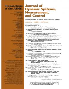
Closed-Form Representation of Beam Response to Moving Line Loads Lu Sun Department of Civil Engineering, The University of Texas at Austin, ECJ Hall 6.10, Austin, TX 78712 e-mail: [email protected] Fig. 3 Variation of the nondimensional stresses S RR and S as functions of the radial distance r on the surface when t Ä0.05 s. Solid line with marks is S RR when there is no coating and the substrate is filled with the same material as coating.
⫽5910 m/s,  1 ⫽3160 m/s, density 1 ⫽6590 kg/m3 ; for substrate, E 2 ⫽6.74⫻1010 N/m2 , ␣ 2 ⫽4150 m/s,  2 ⫽2220 m/s, 2 ⫽5270 kg/m3 . The substrate material is Zinc-Selenide. In Blowers’ paper, the only specified material property is Poisson’s ratio , and we use the same value here as ⫽0.3 for both coating and substrate, for which case a⫽2.017. In Fig. 2, we plot a snapshot of the nondimensional stress S RR at 0.05 s. There is a sharp peak near the surface, which corresponds to the Rayleigh wavefront at r⫽224 m (R⫽(T⫹a 2 )/a ⫽5.84). The boundary of the impact is r⫽213 m (R⫽2 冑T ⫽5.56). In Fig. 3, we show the stresses S RR and S at the surface as functions of the radial distance, in which the symbols ‘‘B,’’ ‘‘R,’’ and ‘‘L’’ mean the boundary of impact area, Rayleigh wavefront, and longitudinal wavefront, respectively. For comparison, we also show the stress S RR when there is no coating and the half-space is filled with the same material as the coating.
Concluding Remarks It was shown that the pressure model in Eq. 共1兲 produces an annular strip of the high tensile stresses outside the contact area due to the Rayleigh wave, which has been observed experimentally by Hand et al. 关7兴. The location and singular behavior of the Rayleigh wavefront are determined from the pressure model and independent of the coating thickness. The region directly under the contact area is in pure compression. Since the stresses cannot have infinite magnitude in real impact situations, the singularity in the present study may be due to the abrupt change of pressure model at the impact boundary.
Acknowledgment The authors would like to thank the Ministry of Science and Technology, Korea, for the financial support by a grant from the Critical Technology 21 Project.
References 关1兴 Evans, A. G., Ito, Y. M., and Rosenblatt, M., 1980, ‘‘Impact Damage Thresholds in Brittle Materials Impacted by Water Drops,’’ J. Appl. Phys., 51, No. 5, pp. 2473–2482. 关2兴 Adler, W. F., 1995, ‘‘Waterdrop Impact Modeling,’’ Wear, 186–187, pp. 341–351. 关3兴 Blowers, R. M., 1969, ‘‘On the Response of an Elastic Solids to Droplet Impact,’’ J. Inst. Math. Appl., 5, No. 2, pp. 167–193.
348 Õ Vol. 68, MARCH 2001
Fourier transform is used to solve the problem of steady-state response of a beam on an elastic Winkler foundation subject to a moving constant line load. Theorem of residue is employed to evaluate the convolution in terms of Green’s function. A closedform solution is presented with respect to distinct Mach numbers. It is found that the response of the beam goes to unbounded as the load travels with the critical velocity. The maximal displacement response appears exactly under the moving load and travels at the same speed with the moving load in the case of Mach numbers being less than unity. 关DOI: 10.1115/1.1352064兴
1
Introduction
The response of beams to moving loads has been studied extensively over the past several decades 共Fryba 关1兴兲. The investigation of Bernoulli-Euler beams with moving loads includes the work of Kenney 关2兴, Steele 关3兴, Huang 关4兴, Choros and Adams 关5兴, Jezequel 关6兴, Elattary 关7兴, Lee 关8兴, Sun and Deng 关9兴, Sun 关10兴, Sun and Greenberg 关11兴, and Benedetti 关12兴. It is found that the moving load is often treated as a concentrated load. Since the concentrated loading condition is only an idealized model of the tire load, it is preferable to use a distributed line load model to characterize the wheel load more realistically. Denote y(x,t) as the deflection of the beam in y-direction, in which x represents the traveling direction of the pavement structure, and t represents time. The well-known governing equation of a Bernoulli-Euler beam on a Winkler foundation is 共Sun 关10兴兲
EI
H 关 r 20 ⫺ 共 x⫺ v t 兲 2 兴 4y 2y 4 ⫹Ky⫹m 2 ⫽P x t 2r 0
(1)
where EI is the rigidity of the beam, E is Young’s modulus of elasticity, I is the moment of inertia of the beam, K is the modulus of subgrade reaction, m is the unit mass of the beam, r 0 is the half-width of the line load, P is the magnitude of the applied load, and H(•) is the Heaviside step function. The Green’s function of the beam is defined as the solution of Eq. 共1兲 given that the right-hand side external load is characterized by ␦ (x⫺x 0 ) ␦ (t⫺t 0 ). Taking two-dimensional Fourier transform and inverse on both sides of Eqs. 共1兲 gives the Green’s function Contributed by the Applied Mechanics Division of THE AMERICAN SOCIETY OF MECHANICAL ENGINEERS for publication in the ASME JOURNAL OF APPLIED MECHANICS. Manuscript received and accepted by the ASME Applied Mechanics Division, Jan. 25, 2000; final revision, Oct. 26, 2000. Associate Editor: A. K. Mal.
The solution of 共1兲 given F(x,t) is given by y(x,t) ⬁ ⬁ 兰 ⫺⬁ F(x 0 ,t 0 )G(x,t;x 0 ,t 0 )dx 0 dt 0 . Substituting Eqs. 共1兲 ⫽ 兰 ⫺⬁ and 共2兲 into it gives ¯P ⬁ sin r exp关 i 共 x⫺ v t 兲兴 0 y 共 x,t 兲 ⫽ (3) ¯ 兲 d 2 ⫺⬁ r 0 共 4 ⫺m ¯ v 2 2 ⫹K
冕
¯ ⫽K/EI and m ¯ ⫽m/EI. where ¯P ⫽ P/EI, K
2
Closed-Form Representation of the Solution
Expression 共3兲 can be further developed using complex function theory. To do so, one needs to identify the roots of the char¯ ⫺m ¯ v 2 2 ⫽0. Define a new acteristic equation of this type 4 ⫹K 2 variable u⫽ so we have a quadratic equation ¯ ⫽0. ¯ v 2 u⫹K (4) u 2 ⫺m ¯ /m ¯ 2 ) 1/4. Define dimenDenote the critical velocity as v critical⫽(4K sionless velocity 共i.e., the Mach number兲 M ⫽ v / v critical . 共a兲 Subsonic case (M ⬍1). ¯ v 2 (1⫹i 冑M ⫺4 ⫺1) 兴 /2 and u 2 Two roots of Eq. 共4兲 are u 1 ⫽ 关 m ¯ v 2 (1⫺i 冑M ⫺4 ⫺1) 兴 /2. Further, we have four complex val⫽关m ¯ v 2 /2M 2 ) 1/2 exp关i(2j⫹)/2兴 and 3,4 ued roots 1,2⫽(m 2 2 1/2 ¯ ⫽(m v /2M ) exp关i(2j⫺)/2兴 in which tan ⫽(M ⫺4⫺1) and j⫽0 and 1. In the case of x⫺ v t⭓0, we select the closed contour in the upper half -plane and, if x⫺ v t⬍0, in the lower half -plane. To shorten the length of the paper, only the case x⫺ v t ⭓0 is considered in the following. Applying the theorem of residue we obtain p sin r 0 exp关 i 共 x⫺ v t 兲兴 y 共 x,t 兲 ⫽ 2i res ¯兲 2 EIr 0 ¯ v 2 2 ⫹K 共 4 ⫺m Im ⬎0
再
⫹i
兺
Im ⫽0
兺
res
再
再
sin r 0 exp关 i 共 x⫺ v t 兲兴 ¯兲 ¯ v 2 2 ⫹K 共 4 ⫺m
冎冎
冎
.
(5)
After identifying the residues in Eq. 共5兲, it is straightforward to see iP sin r 0 l exp关 i l 共 x⫺ v t 兲兴 y 共 x,t 兲 ⫽ . (6) ¯ EIr 0 l⫽1,4 ¯ v 2 l2 ⫹K 5 l4 ⫺m
兺
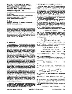
共b兲 Sonic case (M ⫽1). ¯ v 2 /2. In this case two duplicated roots of Eq. 共5兲 are u 1,2⫽m 2 1/2 ¯ Thus four real valued roots 1,2⫽ 3,4⫽⫾(m v /2) . Since these two poles are of the second order, this means that a singularity occurs when integrating 共4兲 along the contour. Using the same procedure as in the case of M ⬍1, it is found that dynamic response in this case becomes infinite and the singularity is of the order O( ⫺1 ). This result indicates the existence of a resonance phenomenon as v ⫽ v critical . 共c兲 Supersonic case (M ⬎1). ¯ v 2 (1⫹ 冑1⫺M ⫺4 ) 兴 /2 and u 2 Two roots of Eq. 共4兲 are u 1 ⫽ 关 m 2 ⫺4 ¯ v (1⫺ 冑1⫺M ) 兴 /2. Therefore, we have real valued roots ⫽关m ¯ v 2 关 1⫹(1 1,2⫽⫾R 1 and 3,4⫽⫾R 2 where R 1⫽ 兵m ¯ v 2 关 1⫺(1⫺M ⫺4 ) 1/2兴 /2其 1/2. Appar⫺M ⫺4 ) 1/2兴 /2其 1/2 and R 2 ⫽ 兵 m ently, since the distribution of the roots of the characteristic equation depends heavily on the range of the Mach number, one may expect that dynamic response of the beam to a moving load will also be distinct for different Mach number. The poles of a system without damping can be thought of as the limit situation of poles of a system with damping while the damping is approaching zero. The poles of a physical system with tiny damping can be determined by seeking the roots of a new characteristic algebraic equation in which a negative infinitesimal imaginary term is added into the previous characteristic algebraic ¯ ⫺i⫽0 where is a positive infini¯ v 2 2 ⫹K equation, i.e., 4 ⫺m tesimal real number. Since u⫽ 2 . This new characteristic equation becomes ¯ ⫺i⫽0. ¯ v 2 u⫹K u 2 ⫺m (7) ¯ v 2 (1 The square root of the discriminant of Eq. 共7兲 is ⌬ 1/2⫽m ⫺4 1/2 ⫺4 ⫺1 ⫺M ) exp(i/2), in which tan ⫽(1⫺M ) and  ¯ ⫺2 v ⫺4 . Since  →0 ⫹ as →0 ⫹ , we have →0 ⫹ and u 1 ⫽4m ¯ v 2 关 1⫹(1⫺M ⫺4 ) 1/2兴 exp(i1) and u 2 ⫽1/2m ¯ v 2 关 1⫺(1 ⫽1/2m ⫺4 1/2 ⫺M ) 兴 exp(i2) as two roots, in which tan 1⫽(1 ⫺M ⫺4)1/2 sin /2/1⫹(1⫺M ⫺4 ) 1/2 cos /2 and tan 2⫽⫺(1 ⫺M ⫺4)1/2 sin /2/1⫺(1⫺M ⫺4 ) 1/2 cos /2, respectively. Thus 1,2⫽R 1 exp关i(1⫹2j)/2兴 and 3,4⫽R 2 exp关i(2⫹2j)/2兴 , ( j ¯ v 2 关 1⫾(1⫺M ⫺4 ) 1/2兴 /2其 1/2. Realize 1 ⫽0,1) where R 1,2⫽ 兵 m ⫽lim →0 ⫹ arctan(tan 1)⫽0⫹ and 2 ⫽lim →0 ⫹ arctan(tan 2) ⫽0⫺, as →0 ⫹ , the roots 1 , 2 , 3 , and 4 , respectively, ap0⫹
/2
proach their own limits arg 1,2⫽ 兵 1⫹ /2⫽ 兵 ⫹0 ⫹ and arg 3,4 1
0⫺
/2
⫽ 兵 2⫹ /2⫽ 兵 ⫹0 ⫺ . 2
Fig. 1 Poles of the beam on an elastic foundation with tiny amount of damping
Journal of Applied Mechanics
MARCH 2001, Vol. 68 Õ 349
Figure 1 depicts the distribution of these poles in the complex -plane. As v approaches critical velocity v critical 共i.e., M →1兲, four poles 共black points兲 will move towards those poles 共gray points兲 of the case v ⫽ v critical . Each pair of gray points on one side of the imaginary axis will get more and more close to each other as M →1, and becomes a single pole of the second order. The dynamic response of the bean is given by y 共 x,t 兲 ⫽
sin r 0 l exp关 i l 共 x⫺ v t 兲兴 iP ¯ 2EIr 0 l⫽1,4 ¯ v 2 l2 ⫹K 5 l4 ⫺m
兺
for x⫺ v t⭓0.
(8) In the case of x⫺ v t⬍0, we just need to replace l⫽1,4 in Eq. 共6兲 or 共8兲 by l⫽2,3.
3
Maximum Response
Define ⫽x⫺ v t. The derivative of y(x,t) with respect to suggests that ⫽0 correspond to the extreme point. The maximum response in the case of M ⬍1 can be obtained by substituting x ⫺ v t⫽0 into Eq. 共7兲. Define new parameters. The maximum removing (x⫽ v t)⫽i P/EIr 0 兵 sin关r exp(i/2) 兴 /S 1 ⫹iW 1 sponse is y max ⫹sin兵r exp关i(⫺⫹)/2兴 其 /S 2 ⫹iW 2 其 in which S 1 ⫽5 4 cos 2 ¯, ¯, ¯ v22 cos ⫹K ¯ v22 cos ⫹K ⫺3m S 2 ⫽5 4 cos 2⫹3m W1 4 2 2 4 ¯ v sin , and W 2 ⫽5 sin 2⫹3m ¯ v22 sin , ⫽5 sin 2⫺3m ¯ v 2 /2M 2 ) 1/2 and r⫽ r 0 . Using Maclaren series to expand ⫽(m moving y max (x⫽ v t) and taking only the real part moving y max 共 x⫽ v t 兲 ⫽⫺
关9兴 Sun, L., and Deng, X., 1997, ‘‘Transient Response for Infinite Plate on Winkler Foundation by a Moving Distributed Load,’’ Chin. J. Appl. Mech., 14, No. 2, pp. 72–78. 关10兴 Sun, L., 1998, ‘‘Theoretical Investigations on Vehicle-Ground Dynamic Interaction,’’ Final Report prepared for National Science Foundation of China, Southeast University, Nanjing, China. 关11兴 Sun, L., and Greenberg, B., 2000, ‘‘Dynamic Response of Linear Systems to Moving Stochastic Sources,’’ J. Sound Vib., 229, No. 4, pp. 957–972. 关12兴 Benedetti, G. A., 1974, ‘‘Dynamic Stability of a Beam Loaded by a Sequence of Moving Mass Particles,’’ ASME J. Appl. Mech., 41, pp. 1069–1071.
再
A 1 S 1 ⫺B 1 W 1 A 2 S 2 ⫺B 2 W 2 P ⫹ EIr 0 S 21 ⫹W 21 S 22 ⫹W 22
冎
(9)
An Analytic Algorithm of Stresses for Any Double Hole Problem in Plane Elastostatics Lu-qing Zhang Engineering Geomechanics Laboratory, Institute of Geology and Geophysics, Chinese Academy of Sciences, Beijing 100029, China
Ai-zhong Lu Professor, Department of Civil Engineering, Shandong University of Science and Technology, Tai’an 271019, China
where ⬁
A 1⫽ B 1⫽
兺
共 ⫺1 兲 n r 2n⫹1 sin关 共 2n⫹1 兲 /2兴 , 共 2n⫹1 兲 !
⬁
共 ⫺1 兲 n r 2n⫹1 cos关 共 2n⫹1 兲 /2兴 , 共 2n⫹1 兲 !
n⫽0
兺
n⫽0 ⬁
A 2⫽
兺
n⫽0
r 2n⫹1 cos关 共 2n⫹1 兲 /2兴 共 2n⫹1 兲 !
and
1
⬁
r 2n⫹1 sin关 共 2n⫹1 兲 /2兴 B 2⫽ . 共 2n⫹1 兲 ! n⫽0 It should be noted that, although ⫽0 can make d/d y⫽0 satisfied, it is a sufficient condition rather than a necessary condition. Actually, the response of the beam at the center of the moving load is the maximal response in the case of M ⬍1, while the response of that location remains quiescent in the case of M ⬎1. It also should be pointed out that similar method is applicable to moving load problem with damping considered in the governing equation. Given the limit of the content, the result is not presented herein.
兺
References 关1兴 Fryba, L., 1977, Vibration of Solids and Structures Under Moving Loads, Noordhoff, Groningen, The Netherlands. 关2兴 Kenney, J. T., 1954, ‘‘Steady State Vibrations of Beam on Elastic Foundation for Moving Loads,’’ ASME J. Appl. Mech., 21, pp. 359–364. 关3兴 Steele, C. R., 1967, ‘‘The Finite Beam With a Moving Load,’’ ASME J. Appl. Mech., 34, p. 111. 关4兴 Huang, C. C., 1977, ‘‘Traveling Loads on a Viscoelastic Timoshenko Beam,’’ ASME J. Appl. Mech., 44, pp. 183–184. 关5兴 Choros, J., and Adams, G. G., 1979, ‘‘A Steadily Moving Load on an Elastic Beam Resting on a Tensionless Winkler Foundation,’’ ASME J. Appl. Mech., 46, No. 1, pp. 175–180. 关6兴 Jezequel, L., 1981, ‘‘Response of Periodic Systems to a Moving Load,’’ ASME J. Appl. Mech., 48, pp. 613–618. 关7兴 Elattary, M. A., 1991, ‘Moving Loads on an Infinite Plate Strip of Constant Thickness,’’ J. Phys. D: Appl. Phys., 24, No. 4, 541–546. 关8兴 Lee, H. P., 1994, ‘‘Dynamic Response of a Beam With Intermediate Point Constraints Subject to a Moving Load,’’ J. Sound Vib., 171, No. 3, pp. 361– 368.
350 Õ Vol. 68, MARCH 2001
This paper gives an analytic algorithm to plane elastostatic problem of an infinite medium containing two holes of arbitrary shapes and arrangement, using Schwarz’s alternating method, and finds that the method has a very quick convergence speed even for solving a complex double hole problem. 关DOI: 10.1115/1.1352065兴
Introduction
There are a large number of papers in plane elastostatics dealing with regions containing two circular holes 共关1–4兴兲. It seems that only Hasebe et al. 关5兴 provided one analysis method for the problem of two complex holes in which one hole is of complex profile and the other is a crack. However, the method is only suitable for a symmetrical double hole problem. The crucial ingredient in solving a double hole problem by means of Schwarz’s alternating method is the repeated solution of a single hole problem, which can be well solved by Muskhelishvili’s method 共关6兴兲 via a conformal transformation of mapping the given hole shape into a unit circle. The iterative solutions for the Schwarz’s alternating method needs many repeated transformations between the physical and mapped planes. In order to conduct the iterative solutions easily, two mapping functions of two holes, z 1 ⫽ 1 ( 1 ) and z 2 ⫽ 2 ( 2 ), and two corresponding inverse map⫺1 ping functions, 1 ⫽ ⫺1 1 (z 1 ) and 2 ⫽ 2 (z 2 ), are introduced. In the process of iterative solutions every iteration refers to the completion of solutions for two single hole problems.
2 Basic Formulas for Stress Analysis of Any Double Hole Problem In Fig. 1 z 1 and z 2 are the complex coordinates in x 1 o 1 y 1 and x 2 o 2 y 2 local coordinate systems, respectively; c is the relative Contributed by the Applied Mechanics Division of THE AMERICAN SOCIETY OF MECHANICAL ENGINEERS for publication in the ASME JOURNAL OF APPLIED MECHANICS. Manuscript received by the ASME Applied Mechanics Division, Mar. 22, 2000; final revision, Sept. 20, 2000. Associate Editor: J. R. Barber.
where a prime on a function denotes differentiation with respect to its argument, and a bar on a function indicates its conjugate; 1 is the value of 1 on the unit circle; 11( 1 ) and 11( 1 ) are the values of 11( 1 ) and 11( 1 ) on the unit circle, respectively; f 1 ( 1 ) is the principal vector of surface forces at the edge of hole one. The stress functions 11( 1 ) and 11( 1 ) can be used as the loading functions for solving another single hole problem induced by the presence of hole two. At this stage the boundary conditions are satisfied at the edge of hole one, however, there exist redundant surface forces at the edge of hole two. The redundant surface forces are obtained directly by three coordinate transformations between coordinates 2 , z 2 , z 1 and 1 and a formula f 12共 2 兲 ⫽ 11共 ␥ 1 兲 ⫹ Fig. 1 The calculating model for any double hole problem
1共 ␥ 1 兲 ⬘1 共 ␥ 1 兲
⬘11共 ␥ 1 兲 ⫹ 11共 ␥ 1 兲
(2)
where 2 is the value of boundary point t 2 of hole two in 2 plane; f 12( 2 ) is the principal vector of the redundant surface forces with respect to 2 ; ␥ 1 is the coordinate of 2 in 1 plane via mapping transformation t 2 ⫽ 2 ( 2 ), coordinate translation T 1 ⫽t 2 ⫹c and inverse mapping transformation ␥ 1 ⫽ ⫺1 1 (T 1 ). The distribution of f 12( 2 ) at the edge of hole two can be L
approximated by complex series
兺 D k k2 , in which D k is the k⫽⫺L
complex coefficient of k2 . In order to eliminate the redundant surface forces, the reversed forces of Fig. 2 The problem for two circular holes
position vector of two holes in x 1 o 1 y 1 coordinate system; ⬁x , ⬁ ⬁y , and xy are external loads uniformly distributed at infinity. In the process of the first iteration, the presence of hole one will lead to a single hole problem, whose solution of stresses can be written in terms of two complex stress functions, 11( 1 ) and 11( 1 ), of the complex variable 1 . The stress boundary condition for the presence of hole one is
L
L
k⫽⫺L
k⫽⫺L
兺 D k k2 , ⫺ 兺 D k k2 ,
are imposed at the edge of hole two, yielding the other single hole problem in the first iteration. The solution for the presence of hole two can be expressed by two complex stress functions 22( 2 ) and 22( 2 ). The corresponding stress boundary condition is
22共 2 兲 ⫹
2共 2 兲 2⬘ 共 2 兲
L
⬘22共 2 兲 ⫹ 22共 2 兲 ⫽ f 2 共 2 兲 ⫺
兺
D k k2
k⫽⫺L
(3)
Table 1 The comparison of the maximum tensile stresses at the edge of the right hole from two methods
Journal of Applied Mechanics
MARCH 2001, Vol. 68 Õ 351
where 22( 2 ) and 22( 2 ) are the values of 22( 2 ) and 22( 2 ) on the unit circle in 2 plane, respectively; f 2 ( 2 ) is the principal vector of surface forces at the edge of hole two. The superposition of 11( 1 ), 11( 1 ) and 22( 2 ), 22( 2 ) is the solution for the first iteration of the Schwarz’s alternating method. At this stage, the boundary conditions only at the edge of hole two are satisfied. Of course, the second and later iterations can be operated. Taking 共兲 and 共兲 as the superposition of two stress functions for all required iterative solutions, the stress components can be obtained readily.
3 Discussions on the Convergence Accuracy of Iterative Solutions
Fig. 3 The problem for two complex holes
3.1 Comparison With the Exact Solution for the Problem of Two Circular Holes. Now let us consider a linearly elastic medium containing two equal circular holes, as plotted in Fig. 2. Three fundamental loading cases are discussed in some detail, namely, the all-around, horizontal and vertical tensions applied at infinity. Owing to the symmetry of the problem, Table 1 only
Fig. 4 The redundant surface forces and for different iterations
Table 2 The maximum compressive stresses at the edges of two holes
352 Õ Vol. 68, MARCH 2001
Transactions of the ASME
gives the maximum tensile stresses on the boundary of the right hole in which the iterative solutions are obtained by the Schwarz’s alternating method for ten iterations and the exact one given by Ling 关3兴. 3.2 Accuracy Analysis for the Problem of Two Complex Holes. Let us consider the problem of an infinite and linearly elastic region, containing two complex holes, only under the action of compressive stresses at infinity 共 ⬁x ⫽10 MPa and ⬁y ⫽20 MPa兲 共see in Fig. 3兲. If the solution is terminated at some iteration, the boundary condition of zero surface forces along hole two will be satisfied exactly and along hole one approximately. Figure 4 plots the distribution of redundant surface forces along hole one for 3, 5, 10, 15, and 20 iterative solutions, seen from which the redundant surface forces are gradually reduced to zeroes as the further iteration.
4 The Maximum Stresses Around Two Holes for Different Loads and Arrangements This paper still takes two holes in Fig. 3 as examples, only changing the loads at infinity and arrangement of the two holes. Three loading cases and three arrangement cases are investigated, and the maximum stresses at the edges of two holes are presented in Table 2.
Acknowledgment
momentum. We find the differential equation of the tautochrone curves. While this differential equation is difficult to solve analytically, several exact solutions (in terms of elementary functions) are obtained in an indirect manner. Intuitive motivation for tautochrone motion is given. 关DOI: 10.1115/1.1352066兴
1
Introduction
Consider a bead of unit mass that moves on a frictionless wire described by the curve x⫽x(y) in the xy-plane. Assume that the bead starts at time t⫽0 at the point (x(Y ),Y ) with no initial velocity and that the curve x⫽x(y) terminates on the x-axis at the point (x 0 ,0). The motion of the bead is governed by a potential V(y) as it moves along the curve x⫽x(y). This curve is called a tautochrone if the time T required for the motion from the starting point at (x(Y ),Y ) to the final point (x 0 ,0) is independent of Y, 共the starting height on the curve兲. The problem of determining the shape of the tautochrone curve under the gravitational potential V(y)⫽gy was solved by Huygens and by Abel. The authors studied this problem under arbitrary potentials V(y) in a recent paper 共关1兴兲 using the fractional calculus. In this paper we assume that the xy-plane containing our curve x⫽x(y) is rotating with constant angular momentum L about a shaft centered on the y-axis. In our previous study 共关1兴兲 共angular velocity ⫽0兲 we determined that the time T for the bead to descend from y⫽Y to y ⫽0 is given by
冕冑
This paper is supported by the Chinese National Natural Science Foundation 共No. 49772166兲.
Y
0
References 关1兴 Howland, R. C. J., and Knight, R. C., 1939, ‘‘Stress Functions for a Plate Containing Groups of Circular Holes,’’ Philos. Trans., 238, pp. 357–392. 关2兴 Green, A. G., 1940, ‘‘General Biharmonic Analysis for a Plate Containing Circular Holes,’’ Proc. R. Soc. London, Ser. A, 176, pp. 121–139. 关3兴 Ling, Chin-bing, 1948, ‘‘On the Stresses in a Plate Containing Two Circular Holes,’’ J. Appl. Phys., 19, pp. 77–82. 关4兴 Ukadgaonker, V. G., 1982, ‘‘Stress Analysis of a Plate Containing Two Circular Holes Having Tangential Stresses,’’ AIAA J., 20, pp. 125–128. 关5兴 Hasebe, N., Yoshikawa, K., Ueda, M., and Nakamura, T., 1994, ‘‘Plane Elastic Solution for the Second Mixed Boundary Value Problem and Its Application,’’ Archive of Applied Mechanics, 64, pp. 295–306. 关6兴 Muskhelishvili, N. I., 1953, ‘‘Some Basic Problems of Mathematical Theory of Elasticity,’’ P. Noordhoff, Groningen, The Netherlands.
⫽ 冑2T.
(1)
Here s measures the distance along the curve x⫽x(y) starting from (x 0 ,0) to the point (x(y),y). Using the fractional calculus we determined that when the curve is a tautochrone, then the potential and the arc length are related by V共 y 兲⫽
2 2 s . 8T 2
(2)
We also determined that the differential equation satisfied by the tautochrone curve is 1⫹x ⬘ 共 y 兲 2 ⫽
2T 2 V ⬘ 共 y 兲 2 . 2 V共 y 兲
(3)
For 共3兲 to be valid, we require that V(0)⫽0. 共This can always be achieved by simply adding a constant to the potential.兲 The solution for our tautochrone curve in terms of the given potential is
In a recent paper by Flores and Osler, the authors investigated tautochrone curves in the xy-plane under an arbitrary potential V(y). In this paper we imagine that the xy-plane of the tautochrone curve is rotating about the y-axis with constant angular Contributed by the Applied Mechanics Division of THE AMERICAN SOCIETY OF MECHANICAL ENGINEERS for publication in the ASME JOURNAL OF APPLIED MECHANICS. Manuscript received by the ASME Applied Mechanics Division, Apr. 2, 2000; final revision, Oct. 9, 2000. Associate Editor: A. A. Ferri.
2T 2 V ⬘ 共 u 兲 2 ⫺1du⫹x 0 . 2 V共 u 兲
(4)
We will use the above results when we solve our rotating tautochrone problem.
2
E. Flores
Journal of Applied Mechanics
ds V 共 Y 兲 ⫺V 共 y 兲
The Rotating Versus Nonrotating Tautochrones
The sum of the kinetic and potential energies for the rotating parts and for our bead of unit mass on the wire x⫽x(y) in the rotating xy-plane 共angular velocity (y)兲 is 1 1 I 共 Y 兲 2 ⫹ 共 Y 兲 2 x 共 Y 兲 2 ⫹V 共 Y 兲 2 2 ⫽
冉 冊
1 ds 2 dt
2
⫹
1 1 I 共 y 兲 2 ⫹ 共 y 兲 2 x 共 y 兲 2 ⫹V 共 y 兲 . 2 2
(5)
The following are important features of 共5兲: A The wire and rotating ‘‘parts’’ are rigid and rotating freely 共without torque兲 about the y-axis. 共See Fig. 1.兲 B On the left of 共5兲 we see the energy at the moment the bead is released at the point (X,Y ) and on the right we see the energy when the bead is at the arbitrary point (x,y) on the wire.
x⫽x(y) is a nonrotating tautochrone under the potential V (y), * then we know that the same curve is a tautochrone rotating with angular velocity (y) under the potential 1 V 共 y 兲 ⫽V 共 y 兲 ⫺ 共 I⫹x 共 y 兲 2 兲 共 y 兲 2 . * 2
(11)
We can eliminate (y) from 共11兲 by using the conservation of angular momentum expressed as L⫽ 共 I⫹x 共 Y 兲 2 兲 共 Y 兲 ⫽ 共 I⫹x 共 y 兲 2 兲 共 y 兲 .
(12)
We require that this angular velocity vary with the starting height Y so as to keep the angular momentum L constant. Solving 共12兲 for (y) and substituting into 共11兲 we get 1 L2 V 共 y 兲 ⫽V 共 y 兲 ⫺ . * 2 共 I⫹x 共 y 兲 2 兲
Fig. 1 The rotating frictionless wire with supports
C The wire is given an initial angular velocity and the bead is started with zero velocity relative to the rotating frame. In particular, at time t⫽0 the system is rotating with angular velocity (Y ) about the y-axis. D As a consequence of C, at time t⫽0 the bead has no component of velocity tangent to the curve but it does have a component of velocity perpendicular to the xy-plane given by (Y )x(Y ). E During the motion the angular velocity of the bead 共and the system of parts兲 given by (y) will vary. It will change so that angular momentum is always conserved. 共See relation 共12兲兲. F The moment of inertia of the wire, rotating shaft and supports is I and its kinetic energy is the term 1/2I (y) 2 . G The term ds/dt is the magnitude of the velocity component tangent to the curve. The arc length s is measured from the terminal point (x 0 ,0) to the moving point (x(y),y). If we call V (y) the terms * 1 1 V 共 y 兲 ⫽V 共 y 兲 ⫹ I 共 y 兲 2 ⫹ 共 y 兲 2 x 共 y 兲 2 , (6) * 2 2 we can abbreviate the writing of 共5兲 as simply
冉 冊
1 ds V 共 Y 兲 ⫽V 共 y 兲 ⫹ * * 2 dt
2
.
(7)
We recall from our previous paper that all the potentials we use are required to satisfy V(0)⫽V (0)⫽0 so that relations 共1兲 to 共4兲 * are all valid. Since x(0)⫽x 0 we must add the constant term 2 2 L /2(I⫹x 0 ) to the right side of 共13兲 so that all potentials are zero when y⫽0. We get 1 L2 L2 V 共 y 兲 ⫽V 共 y 兲 ⫺ ⫹ . 2 * 2 共 I⫹x 共 y 兲 兲 2 共 I⫹x 20 兲
(8)
The minus sign in 共8兲 is due to the assumption that the arc length s is decreasing. This requires that the initial angular speed (Y ) be small enough that when the bead is released with zero relative velocity, the bead falls downward instead of flying outward. For example, in the case of a gravity-potential, it assumes that
We will use 共14兲 to find several rotating tautochrones in the next section.
3
We can now write ds
. (9) 共 Y 兲 ⫺V 共 y 兲 * * Integrating from the beginning of the motion to the end we get
冑2T⫽
冑V
冕冑 Y
ds
. (10) V 共 Y 兲 ⫺V 共 y 兲 * * Notice that Eqs. 共1兲 and 共10兲 have the same form, thus, they have the same solution. This implies that for a given curve x⫽x(y), the time T for the rotating case under the potential V(y) is the same as the time for the nonrotating case under the potential V (y). This * last statement is important for our work. If we know that the curve 0
354 Õ Vol. 68, MARCH 2001
Finding Exact Rotating Tautochrones
In our previous paper we found exact nonrotating tautochrones indirectly. We started with a curve x⫽x(y) for which we could calculate the arc length s⫽s(y) exactly. We then used relation 共2兲 to find the potential that would make this curve a tautochrone. Nine such curves were selected for their ease of calculation. All nine can be easily modified using 共14兲 to give us rotating tautochrones. The results are shown in Table 1. While all the resulting potentials are bizarre, we believe it is important to collect exact solutions of mechanics problems whenever they are possible. When exact analytic solutions cannot be found, perturbation or numerical solutions are usually possible. The latter tell us much less than the exact solutions.
We will now find the differential equation satisfied by the rotating tautochrone. Relation 共3兲 is the differential equation for the nonrotating tautochrone. Substituting V (y) from 共14兲 for V(y) in * 共3兲 we get 2
1⫹x ⬘ 共 y 兲 2 ⫽
dy x 共 Y 兲 共 Y 兲 2 ⬎ . dx g
冑2dt⫽⫺
(14)
4 The Differential Equation for the Rotating Tautochrone
Solving 共7兲 for ds/dt we get ds ⫽⫺ 冑2 冑兵 V 共 Y 兲 其 ⫺ 兵 V 共 y 兲 其 . * * dt
(13)
2T 2
再
再
冎
L 2x 共 y 兲 x ⬘共 y 兲 2 共 I⫹x 共 y 兲 2 兲 2 . (15) L2 L2 V共 y 兲⫹ 2 ⫺ 2 2 共 I⫹x 共 y 兲 兲 2 共 I⫹x 0 兲 V ⬘共 y 兲 ⫺
冎
This is our differential equation for the rotating tautochrone. It is much more complex and difficult to solve than 共3兲. We can rewrite 共15兲 in the form
2 兵 2 共 I⫹x 20 兲共 I⫹x 共 y 兲 2 兲 V 共 y 兲 ⫺L 2 x 共 y 兲 2 其 共 I⫹x 共 y 兲 2 兲 3 共 1⫹x ⬘ 共 y 兲 2 兲 ⫽4 共 I⫹x 20 兲 T 2 兵 共 I⫹x 共 y 兲 2 V ⬘ 共 y 兲 ⫺L 2 x 共 y 兲 x ⬘ 共 y 兲 其 2 .
(16)
We can use 共15兲 or 共16兲 to check our solutions in Table 1, but solving exactly for a given potential appears to be difficult. Of course, numerical solutions are possible.
5
The Case Where I is Large
We now discuss the approximation where the moment of inertia of the bead, x 2 , is much smaller than I, the moment of inertia of Transactions of the ASME
Table 1 Examples of Potentials and Corresponding Rotating Tautochrone Curves Tautochrone Curve 1
x⫽R sin ⫹x0 , y⫽R⫺R cos circle: center (x 0 ,R), radius R
Arc Length s s⫽R⫽R cos⫺1
Potential V(y)
冉 冊 R⫺y R
⫺ 2
3
4
x⫽R⫺R cos ⫹x0 y⫽R sin circle: center (R⫹x 0 ,0), radius R x⫽R sin(␣⫹)⫺R sin ␣ ⫹x0 y⫽R cos ␣⫺R cos(␣⫹), R and ␣ fixed circle: radius R center (x 0 ⫺R sin ␣,R cos ␣) x⫽R( ⫹sin )⫹x0 y⫽R(1⫺cos ) inverted cycloid: base line y⫽2R
再 冉 冊冎
R R⫺y cos⫺1 8T2 R 2 2
s⫽R ⫽R sin⫺1(y/R))
2共I⫹共冑2Ry⫺y 2 ⫹x 0 兲 2 兲
⫺L2/共2共I⫹共R⫺冑R 2 ⫺y 2 ⫹x 0 兲 2 兲兲
⫽cos⫺1
冉
再 冉 冊 冎
s⫽R R cos共␣兲⫺y ⫺␣ R
2 2R2 a⫺y L2 ⫺1 ⫺␣ ⫹ 2 cos 8T R 2共I⫹x20兲
冊
⫺ s⫽4R sin(/2) s⫽2 冑2Ry
L2 2共I⫹共冑R 2 ⫺ 共 R cos ␣⫺y 兲2⫺R sin ␣⫹x0兲2兲 where a⫽R cos(␣) 2R L2 y⫹ T2 2共I⫹x20兲
冉 再
s⫽4R(1⫺cos(/2)) y s⫽4R 1⫺ 1⫺ 2R
L2
冉 冊冑
冉 冑 冊 冉 再
2 I⫹ R cos⫺1 x⫽ay⫹x 0
7
x⫽2 冑ay 3 /3⫹x 0
s⫽ 冑1⫹a 2 y
s⫽
x⫽ay 2 /2⫹x 0
y⫽a cosh((x⫺x0)/a)⫺a ⫹x0
s⫽ 冑(y⫹a) 2 ⫺a 2
L2 R⫺y ⫺冑2Ry⫺y 2 ⫹x 0 R
冉 冊
L2 2 共 I⫹ 共 2 冑ay 3 /3⫹x 0 兲 2 兲
2
⫹
L2 2 共 I⫹x 20 兲
L2 L2 2 2 ⫹ 2 共 I⫹ 共 ay /2⫹x 0 兲 兲 2 共 I⫹x 20 兲
2 L2 2 2 2 关共 y⫹a 兲 ⫺a 兴⫹ 8T 2共I⫹x20兲
冉冉 再
⫺L2/ 2 I⫹ a cosh⫺1
the wire, shaft and support. We will also assume that x 0 ⫽0, so that the wire is attached directly to the shaft at the bottom. Starting with 共14兲 we can write
冎冊
2 共 ay 冑1⫹a 2 y 2 ⫹ln共ay⫹冑1⫹a 2 y 2 兲兲 2 32a 2 T 2 ⫺
9
2
2 关共 1⫹ay 兲 3/2⫺1 兴 2 18a 2 T 2
2 关共1⫹ay 兲3/2⫺1 兴 3a
s⫽(ay 冑1⫹a 2 y 2 ⫹ ln(ay⫹冑1⫹a 2 y 2 ))/2a
冎冊
2共1⫹a2兲 2 L2 L2 y⫺ ⫹ 8T2 2共I⫹共ay⫹x0兲2兲 2共I⫹x20兲
⫺ 8
R⫺y ⫹ 2Ry⫺y 2 ⫹x 0 R
2R L2 y⫹ T2 2 共 I⫹x 20 兲 ⫺
6
L2 2共I⫹x20兲
L2
2 I⫹ R cos⫺1 x⫽R ⫺R sin ⫹x0 y⫽R⫺R cos cycloid
⫹
2R2 L2 ⫺1 2 2 兵sin 共 y/R 兲其 ⫹ 8T 2共I⫹x20兲
⫺
5
2
冉 冊 冎 冊冊 y⫹a ⫹x0 a
2
1 L2 x共 y 兲2. V 共 y 兲 ⫽V 共 y 兲 ⫺ * 2 I2
L2 L2 V 共 y 兲 ⫽V 共 y 兲 ⫹ ⫺ . 2 * 2I 共 1⫹x 共 y 兲 /I 兲 2I
The conservation of angular momentum 共12兲, to a first-order approximation becomes simply L⫽I where is now a constant. Thus the above expression becomes
Expanding the second term on the right in powers of x(y) 2 /I we obtain to a first-order approximation
1 V 共 y 兲 ⫽V 共 y 兲 ⫺ 2 x 共 y 兲 2 . * 2
Journal of Applied Mechanics
MARCH 2001, Vol. 68 Õ 355
The differential Eq. 共15兲 is now much simpler, 1⫹x ⬘ 共 y 兲 2 ⫽
2T 2 兵 V ⬘ 共 y 兲 ⫺ 2 x 共 y 兲 x ⬘ 共 y 兲 其 2 . 1 2 V共 y 兲⫺ 2x共 y 兲2 2
再
冎
As an example consider the potential of a simple harmonic oscillator V(y)⫽ky 2 /2 and try a straight line solution x(y)⫽ay, the differential equation becomes 共after simplifying兲 1⫹a 2 ⫽
4T 2 兵 k⫺a 2 2 其 . 2
Solving for a we get a⫽ 冑4T 2 k⫺ 2 /4T 2 2 ⫹ 2 . Thus, under a harmonic oscillator potential the tautochrone curve is a straight line with slope a. In general the potential for the rotating tautochrone, to a firstorder approximation, is 1 V 共 y 兲 ⫽V 共 y 兲 ⫹ 2 x 共 y 兲 2 ⫹C. * 2
Fig. 3 Why all tautochrones act like simple springs
The first term is the potential of a nonrotating tautochrone V (y), * the second term is the potential of a simple harmonic oscillator, and C is a constant. The second term could be produced by an ideal spring stretched along the x-axis with one end attached to the bead and at the other to the shaft. As the bead moves down so does the spring. The tension in the spring serves to exactly cancel the centrifugal force 2 x. Thus, the motion of the bead along the wire, as seen by an observer rotating with the system, will be identical to the motion of the bead of a nonrotating tautochrone of potential V (y). *
6
2 V 共 y 兲⫽ 2 s 2. * 8T Next use 共14兲 to replace V (y) to obtain * 1 L2 2 2 L2 V共 y 兲⫹ s . 2 ⫺ 2 ⫽ 2 共 I⫹x 共 y 兲 兲 2 共 I⫹x 0 兲 8T 2 Differentiate with respect to y and get V ⬘共 y 兲 ⫺
Physical Intuition Behind Tautochrones
There is a simple, beautiful explanation for all tautochrone motion. All tautochrones act like simple linear springs. Suppose a mass m attached to a spring is displaced a distance A from equilibrium. The time required for the mass to return to the equilibrium position is T⫽
2
冑
m k
(17)
where k is the spring constant. This time is independent of the displacement A and thus we have tautochrone motion in every simple spring. The restoring force from the spring is proportional to the distance s that the spring is stretched: F⫽ks. Solving 共17兲 for k we can write this force as m s. 4T 2
From 共12兲 we see that (y) 2 ⫽L 2 /(I⫹x(y) 2 ) 2 and thus the above expression can be written as V ⬘ 共 y 兲 ⫺x 共 y 兲 共 y 兲 2
dx 2 ds ⫽ 2s . dy 4T dy
Finally we multiply by dy/ds to get V ⬘共 y 兲
dy dx 2 ⫺x 共 y 兲 共 y 兲 2 ⫽ 2 s. ds ds 4T
From Fig. 2 we see that the derivatives in the above expression can be replaced by dx/ds⫽cos and dy/ds⫽sin . V ⬘ 共 y 兲 sin ⫺x 共 y 兲 共 y 兲 2 cos ⫽
2
F⫽
L 2x 共 y 兲 x ⬘共 y 兲 2 ds s . 2 2 ⫽ 4T 2 dy 共 I⫹x 共 y 兲 兲
(18)
This formula is also valid for any nonrotating tautochrone 共关2兴兲. Let us now examine the forces on the bead 共of unit mass兲 on our rotating tautochrone curve. Starting with relation 共2兲 and replacing the potential by V (y) we get *
2 s. 4T 2
(19)
Using Fig. 3 we see that the term V ⬘ (y)sin is the component of the force generated by the potential in the direction tangent to the tautochrone curve. We also see that the term x(y) (y) 2 cos is the component of centripetal acceleration along the tautochrone curve. Thus we see that 共19兲 tells us that when the forces acting on our bead are resolved in the direction tangent to the tautochrone curve, then the sum of these forces is proportional to the distance s from the final point on the tautochrone. This is similar to 共18兲 that describes the simple spring. 共Notice that with m⫽1 the constants in 共18兲 and 共19兲 are identical.兲 The sum of the forces tangent to a tautochrone curve on a moving bead is proportional to the distance measured from the final point to the bead.
References
Fig. 2 Geometric meaning of differentials
356 Õ Vol. 68, MARCH 2001
关1兴 Flores, E. V., and Osler, T. J., 1999, ‘‘The Tautochrone Under Arbitrary Potentials Using Fractional Derivatives,’’ Am. J. Phys., 67, pp. 718–722. 关2兴 McKinley, J. M., 1979, ‘‘Brachistochrones, Tautochrones, Evolutes, and Tesselations,’’ Am. J. Phys., 47, No. 1, pp. 81–86.
Transactions of the ASME
Smooth Asymmetric Two-Dimensional Indentation of a Finite Elastic Beam
deformation due to contact pressure and the global flexural deformation of the beam. The validity of the solutions presented is assessed by comparing the results obtained to the predictions of modified beam theory solutions.
Generalized Elasticity Solution for a Finite Layer
M. Zhou Graduate Research Assistant, Civil and Environmental Engineering Department, University of Alabama, Huntsville, AL 35899
W. P. Schonberg Professor and Chair, Civil Engineering Department, University of MissouriRolla, Rolla, MO 65409 Mem. ASME e-mail: [email protected]
Standard methods of beam indentation analysis use a beam theory solution to obtain the load-displacement relationship and a Hertz solution to calculate local stresses. However, when the contact length exceeds the thickness of the beam point contact can no longer be assumed and Hertzian relations are no longer valid. This paper presents an improved superposition solution technique that uses a true elasticity solution to obtain the load-displacement relationship in non-Hertzian indentation problems. 关DOI: 10.1115/1.1352068兴
Introduction
In this section we present the solution for a finite elastic layer of thickness that is subjected to an arbitrary upper surface pressure distribution. This solution is achieved by the superposition of an elasticity solution for an infinite layer loaded on its upper surface with an elasticity solution for a finite layer subjected to asymmetric bending. A suitable elasticity solution that represents normal loading on the upper surface of an infinite elastic layer in plane strain with no loading on its lower surface is given by Keer and Miller 关1兴. To complete the finite elastic layer solution, we introduce the following elasticity solution for the asymmetric bending of a finite layer 共thickness h and length L兲 having end moments M 0 and M 1 :
u x⫽
再 冋
y y ⫽0,
(1)
xy ⫽
V共 x 兲 y 共 h⫺y 兲 , 2I
(2)
xx ⫽
M共x兲 h y⫺ I 2
(3)
冉 冊
1 2⫺ M 1 ⫺M 0 b ⫺a 1 y⫹ 关 2 共 h⫺y 兲 3 ⫺3h 共 h⫺y 兲 2 兴 D 0 12共 1⫺ 兲 L M 1 ⫺M 0 共 L 0 ⫹x 兲 2 2L
⫹ M 0 x⫹ u y⫽
冋
册冉 冊 y⫺
h 2
1 1 M 1 ⫺M 0 a 0 ⫹a 1 x⫺ M 0 x 2 ⫺ 共 L 0 ⫹x 兲 3 D 2 6L
(4)
册
In this paper, we present an improved solution to the twodimensional problem of a finite beam of length L and thickness h that is loaded asymmetrically on its upper surface by a frictionless cylindrical indenter 共see Fig. 1兲. Standard methods of indentation analysis use a beam theory solution to obtain an overall loaddisplacement relationship and then a Hertzian contact solution to calculate local stresses under the indenter. However, previous modeling efforts have shown that the stress distribution in the region of contact will differ significantly from a Hertzian one when the contact length exceeds the thickness of the beam. In such cases, point contact can no longer be assumed and Hertzian relations are not valid. Problems of this type were solved previously by Keer and Miller 关1兴 and Peck and Schonberg 关2兴 using a GLOBAL/LOCAL approach that superposed beam theory and elasticity expressions. The technique developed was also applied to cantilever beam indentation by Keer and Schonberg 关3,4兴 and subsequently modified to include beam rotation effects by Zhou and Schonberg 关5兴. A review of the superposition procedure used by Keer, Schonberg, et al. reveals that it has a problematic aspect: it uses an approximate solution 共instead of an elasticity solution兲 to establish the load-displacement relationship at the contact site. The improved superposition technique presented in this paper addresses this issue by using a static finite layer solution that is a true elasticity solution. Also, in a manner similar to that used by Zhou and Schonberg 关5兴 to model cantilever beam indentation, the rotation of the beam under the indenter is included in the mixed boundary condition at the contact site. As a result, the final solution takes into consideration all of the prescribed boundary and end conditions and describes more accurately the local surface
Asymmetric Beam Indentation Model
Contributed by the Applied Mechanics Division of THE AMERICAN SOCIETY OF MECHANICAL ENGINEERS for publication in the ASME JOURNAL OF APPLIED MECHANICS. Manuscript received and accepted by the ASME Applied Mechanics Division, May 31, 2000; final revision, Oct. 10, 2000. Associate Editor: M.-J. Pindera.
The mixed boundary value problems to be solved in this section are those of a simply supported and a fixed-fixed elastic beam that are indented by a cylindrical punch on their upper surface 共see again Fig. 1兲. The solutions of these problems are achieved by application of the mixed boundary conditions at the contact sites
Journal of Applied Mechanics
⫺ ¯ 共 x 兲 ⬅ 1 h ⫹
冕
M 共 x 兲共 y 2 ⫺hy 兲 2 共 1⫺ 兲 D h
0
冋
M 1 ⫺M 0 uy 1 a 1 ⫺M 0 x⫺ dy⫽ 共 L 0 ⫹x 兲 2 x D 2L
h2 M 1 ⫺M 0 12共 1⫺ 兲 D L M 共 x 兲 ⫽M 0 ⫹
M 1 ⫺M 0 共 L 0 ⫹x 兲 , L
V共 x 兲⫽
M 1 ⫺M 0 L
(5)
册 (6) (7) (8)
where L 0 , L, and L 1 are as shown in Fig. 1, D⫽ h 3 /6(1⫺ ), I⫽h 3 /12, M 0 , M 1 are end bending moments at x⫽⫺L 0 and at x⫽L 1 , respectively, and a 0 , b 0 , a 1 are 共as yet兲 unknown constants. This solution is a superposition of the Airy stress function solutions for asymmetric bending and for pure shear. Superposing Eqs. 共1兲–共8兲 with the corresponding expressions for stresses, displacements, etc., in Keer and Miller 关1兴 yields the generalized elasticity solution for a finite length isotropic elastic layer subjected to an arbitrary upper surface loading. In the next section, we apply appropriate end conditions to this solution to obtain the desired beam indentation problem solutions.
x2 兩 x 兩 ⬍c (9) 2R where ⌬ and 0 are the beam upper surface displacement and rotation under the indenter. The two types of end support conditions that need to be satisfied are 共1兲 simple supports 共zero moment and displacement at the beam ends兲, and 共2兲 fixed ends 共zero slope and displacement at the fixed ends兲. By applying these end support conditions to appropriate expressions in the generalized elasticity solution, we obtain a system of four equations for the four unknowns a 0 , a 1 , M 0 , and M 1 for each beam type. Once solved, the expressions for these four quantities are used in applying the mixed boundary condition at contact site given by Eq. 共9兲. Following the approach used by Keer, Schonberg, et al. we obtain two coupled Fredholm integral equations of the second kind. These equations have the following forms: u y 共 x,0兲 ⫽⌬⫹ 0 x⫺
h3 共 x 兲⫹ 6
冕
c
冕
共 t 兲 K 1 共 x,t 兲 dt⫹
0
h3 共 x 兲⫹ 6
c
共 t 兲 K 2 共 x,t 兲 dt⫹ f 共 x 兲 ⫽⫺
0
冕
c
共 t 兲 K 3 共 x,t 兲 dt⫹
0
冕
c
Dx R (10)
K 2 共 x,t 兲 ⫽
x h3 关 sin共 L 0 兲 ⫹sin共 L 1 兲兴 J 0 共 t 兲 d 6L  ⫺sh 
⫺
3⫺2 h 2 x 1⫺ 12L
h3 6L
冕
⬁
0
K 3 共 x,t 兲 ⫽
(18)
x 关 cos共 L 0 兲 ⫺cos共 L 1 兲兴 J 1 共 t 兲 d  ⫺sh  (19)
冉冊 冕 冉 0
K 4 共 x,t 兲 ⫽0 f 共 x 兲⫽
g 共 x 兲 ⫽⫺
3 x2 共 M 1 ⫺M 0 兲 4 L
⫹
冊
册
x cos共 L 0 兲 ⫹cos共 L 1 兲 共 L 1 ⫺L 0 兲 2 J t d ⫹ x 兲 共 0 2 2 4L (12)
3
K 3 共 x,t 兲 ⫽
h 6
共 L 1 ⫺L 0 兲 xt 4L
冉冊 冕冉 3
h 1 ⫹ t 6
⬁
0
 ⫹sh  ch  ⫹1  2 ⫺sh 2 
(13)
P⫽⫺
M ⫽⫺
3x2 共 L 0 ⫺L 1 兲 8L
358 Õ Vol. 68, MARCH 2001
c
共 t 兲 dt,
(24)
冕
c
t 共 t 兲 dt.
(25)
0
Once Eqs. 共10兲,共11兲 are solved to obtain (x) and (x), all necessary quantities can also be readily obtained. The actual solution of Eqs. 共10兲,共11兲 is performed numerically in nondimensional form. This transformation is obtained using the following nondimensional parameters: L 0 /h, L/h, t/c, x/c, y/h, Rh 3 (x)/Dc, and Rh 3 (x)/Dc, and R⌬/h 2 . To assess the validity of the elasticity solutions, their predictions for beam displacement are compared with the predictions of beam theory solutions that use as input the contact pressure generated by the elasticity solutions. These solutions are given as follows:
⌬ SS ⫽ 3x2 t 8L
L 0L 1 关 L L P⫹ 共 L 1 ⫺L 0 兲 M 兴 3DL 0 1 ⫹
(14)
f 共 x 兲 ⫽0,
冕
Simply Supported Ends.
冊
⫻ 关 J 0 共 x 兲 ⫺ xJ 1 共 x 兲 ⫺1 兴 J 1 共 t 兲 d ⫺
K 4 共 x,t 兲 ⫽⫺
(23)
0
h 3  ⫹sh  ch  ⫹1 xJ 0 共 x 兲 6  2 ⫺sh 2 
K 2 共 x,t 兲 ⫽
(22)
The functions (t) and (t) are related to the symmetric and anti-symmetric components of the surface loading as follows:
共 t 兲 K 4 共 x,t 兲 dt⫹g 共 x 兲 ⫽0
Simply Supported Ends.
0
(20)
(21)
x 共 L ⫺L 0 兲共 M 1 ⫺M 0 兲 , 2L 1
(11)
冕冋 冉
冊
⫻ 关 J 0 共 x 兲 ⫺ xJ 1 共 x 兲 ⫺1 兴 J 1 共 t 兲 d
where the kernels K 1 through K 4 and the functions f (x), g(x) are given as follows:
K 1 共 x,t 兲 ⫽⫺
h 3  ⫹sh  ch  ⫹1 6  2 ⫺sh 2 
⬁
h3 1 ⫹ 6 t
0
⬁
冎
⫺ Fig. 1 Indentation of a finite layer
and the appropriate end support conditions in the generalized elasticity solution presented in the preceding section. As in Zhou and Schonberg 关5兴, the boundary condition for both types of beams at contact sites is written as follows:
冊
h 3  ⫹sh  ch  ⫹1 xJ 0 共 x 兲 6  2 ⫺sh 2 
⬁
(15)
⫹
(16)
Fixed-Fixed Ends.
1 D
冕冉 c
0
冊
L 0L 1 t 2 ⫺ t 共 t 兲 dt 4L 9
共 L 1 ⫺L 0 兲 32DL
冕
c
t 3 共 t 兲 dt
(26)
0
Transactions of the ASME
⌬ FF ⫽⌬ SS ⫺
L 20 L 21 3DL
3
共 L 2 ⫺L 0 L 1 兲 P⫺
L 0L 1 共 L ⫺L 0 兲 6DL 3 1
⫻ 关 L ⫹ 共 L 1 ⫺L 0 兲 2 ⫹L 0 L 1 兴 M 2
⫺ ⫹
L 0L 1 2 关 L ⫹2 共 L 1 ⫺L 0 兲 2 ⫹2L 0 L 1 兴 12DL 3 L 0 L 1 共 L 1 ⫺L 0 兲 16DL 3
冕
c
t 3 共 t 兲 dt
冕
c
t 2 共 t 兲 dt
0
(27)
0
where ⌬ SS is given by Eq. 共26兲, and P, M are again given by Eqs. 共24兲,共25兲, respectively.
Results and Discussion Solutions to the two types of indentation problems were obtained for c/h⫽0.25, 0.5, 1.0 and 2.0, L/h⫽10.0 and 20.0, and for each L/h value, 2L 0 /L⫽1.0, 1.5, and 1.7 共where 2L 0 /L ⫽1.0 corresponds to the case of central indentation studied by Keer and Miller 关1兴兲. We note that for 2L 0 /L⫽1.7 and L/h ⫽10, c/h⫽2.0 would imply that the contact length would extend past the support; hence, c/h⫽2.0 was not considered in this case. For the fixed-fixed beam indentation problem, all calculations are performed with a Poisson’s ratio of 0.3. The results of this parametric study were compared with values obtained using the models developed by Keer and Miller 关1兴 and Peck and Schonberg 关2兴 that did not include upper-surface rotation effects. For small values of c/h 共i.e., c/h⭐0.5兲, the predictions of peak contact stress values by the various solutions agreed quite well. However, for c/h⭓1 the peak stress predictions were found to occasionally differ significantly. This occurred because as c/h increases, the effects of beam upper surface rotation effects become more pronounced. While the current model incorporates those effects, the previous models do not. Therefore, the various models will match more closely for smaller contact areas and indenter locations that result in minimal rotation effects. For larger contact areas and for indenter locations near beam ends, peak contact stress values predicted by the various models differed by as much as 10–15 percent for both types of beam supports. Finally, we
note that while there were differences in peak contact stress values, the overall shapes of the contract stress distributions were very similar to those presented by Keer and Miller 关1兴 and by Peck and Schonberg 关2兴. A comparison between the predictions of beam displacement under the indenter generated by the improved solutions developed herein and the predictions of the beam theory solutions showed that the results of the two solutions agreed very well, and that the agreement improved as L/h increased and c/h decreased. This can be explained by the following considerations. First, as L/h increases, the effects of shear deformation on beam response become negligible. Second, as c/h decreases, the local effects of beam upper surface rotation become negligible. In both cases, while the elasticity solution incorporates those effects, the beam theory solutions do not. Therefore, the two solutions will match more closely for indenter locations that result in minimal shear deformations and for smaller c/h values. Differences between the displacement predictions of the elasticity solution developed herein and the predictions obtained using the GLOBAL/LOCAL models developed previously by Keer and Miller 关1兴 and Peck and Schonberg 关2兴 showed fairly minimal differences for small c/h values and for most 2L 0 /L values 共typically less than five percent兲. This was expected because 共1兲 the governing equations of motion for the solution developed herein and the solutions developed by Keer and Miller 关1兴 and Peck and Schonberg 关2兴 are identical for the case of simply supported ends, and 共2兲 beam upper surface rotation effects on beam response are minimal when for small c/h values. Furthermore, in the case of fixed-fixed beams, as 2L 0 /L→1 and L/h increases, the condition of zero rotation angle at the fixed end supports has less of an effect on the contact zone. Therefore, the effects of second order shearing effects on the average beam rotation ¯ for the new model become negligible. While the current model incorporates those effects, the previous models do not. Therefore, the newly developed and previous models will match more closely for smaller contact area and indenter locations that result in minimal rotation and shearing effects. Figure 2 shows the nondimensional load-displacement curves for L/h⫽10 and 20 fixed-fixed beams where 2L 0 /L⫽1.7. The
Fig. 2 Nondimensional displacement comparisons, new model versus old models „Keer and Miller †1‡; Peck and Schonberg †2‡…, fixed-fixed beams, 2 L 0 Õ L Ä1.7, L Õ h Ä10.0 and 20.0
Journal of Applied Mechanics
MARCH 2001, Vol. 68 Õ 359
larger differences in some of the indentation scenarios shown in this figure can probably be attributed to limitations in the numerical integrations of the infinite integrals that appeared in the work performed by Peck and Schonberg 关2兴. According to Peck and Schonberg, it was not possible to integrate the kernels in the fixed-fixed beam equations to the same accuracy as those in the simply supported cases. This was due to the fact that the kernels for simply supported beam equations converged at a rate of 1/ 2 , while those for the fixed-fixed beams converged at the much slower rate of 1/. In our solution, we have overcome this numerical integration limitation by using exact integration results for expressions involving Bessel functions. This allowed the kernels in the fixed-fixed beam equations to converge at the much faster rate of 1/sh . Interestingly enough, the value of R 共the radius of the indenter兲 did not appear to have any bearing on the solution of the governing equations for this problem. That is, the nondimensional stress and displacement values calculated using the model developed herein would appear to be valid for all values of R! Mathematically, this occurs because of the nondimensional scheme: in this scheme, all traces of R are removed by the nondimensionalization process. However, R does have an effect when the nondimensional values of stress and displacement are transformed into real values. While all of the nondimensional predictions of the model may be mathematically possible, they may not be physically attainable for some values of R. For example, the case of c/h⫽2 is clearly more readily attainable for very large values of R 共as compared to h兲, and significantly less so 共if not impossible兲 for small values of R 共as compared to h兲.
360 Õ Vol. 68, MARCH 2001
Summary and Conclusions The static and dynamic indentation of beams and plates continues to be an intriguing problem, especially for scenarios in which large area contact can be expected to occur. The solution scheme presented herein is a refinement of the approach originally developed for the relatively simple problem of central beam indentation. We found that the results provided by this refinement are, in most cases, not significantly different from those that can be obtained using existing GLOBAL/LOCAL analysis techniques. However, the changes introduced into the modeling process should allow this refined solution technique to more accurately predict internal stress fields due to upper surface indentations. This capability is critical in the case of composite beams or plates where internal damage can appear prior to any evidence of damage on the external beam or plate surface.
References 关1兴 Keer, L. M., and Miller, G. R., 1983, ‘‘Smooth Indentation of a Finite Layer,’’ J. Eng. Mech., 109, pp. 706–717. 关2兴 Peck, J. A., and Schonberg, W. P., 1993, ‘‘Asymmetric Indentation of a Finite Elastically Supported Beam,’’ J. Appl. Mech., 60, pp. 1039–1045. 关3兴 Keer, L. M., and Schonberg, W. P., 1986, ‘‘Smooth Indentation of an Isotropic Cantilever Beam,’’ Int. J. Solids Struct., 22, pp. 87–106. 关4兴 Keer, L. M., and Schonberg, W. P., 1986, ‘‘Smooth Indentation of a Transversely Isotropic Cantilever Beam,’’ Int. J. Solids Struct., 22, pp. 1033–1053. 关5兴 Zhou, M., and Schonberg, W. P., 1995, ‘‘Rotation Effects in the Global/Local Analysis of Cantilever Beam Contact Problems,’’ Acta Mech., 108, pp. 49–62.