Using ASME format

S. J. Sherwin O. Shah D. J. Doorly J. Peiro´ Y. Papaharilaou Biomedical Flow Group, Aeronautics Department, Imperial College, London, SW7 2BY, United Kingdom

N. Watkins C. G. Caro Department of Biological and Medical Systems, Imperial College, London, SW7 2BX, United Kingdom

C. L. Dumoulin GE Corporate Research and Development, Schenectady, NY 12309

1

The Influence of Out-of-Plane Geometry on the Flow Within a Distal End-to-Side Anastomosis This paper describes a computational and experimental investigation of flow in a prototype model geometry of a fully occluded 45 deg distal end-to-side anastomosis. Previous investigations have considered a similar configuration where the centerlines of the bypass and host vessels lie within a plane, thereby producing a plane of symmetry within the flow. We have extended these investigations by deforming the bypass vessel out of the plane of symmetry, thereby breaking the symmetry of the flow and producing a nonplanar geometry. Experimental data were obtained using magnetic resonance imaging of flow within perspex models and computational data were obtained from simulations using a high-order spectral/hp element method. We found that the nonplanar three-dimensional flow notably alters the distribution of wall shear stress at the bed of the anastomosis, reducing the peak wall shear stress peak by approximately 10 percent when compared with the planar model. Furthermore, an increase in the absolute flux of velocity into the occluded region, proximal to the anastomosis, of 80 percent was observed in the nonplanar geometry when compared with the planar geometry. 关S0148-0731共00兲00401-5兴

Introduction

Although arterial bypass grafting is a commonly performed surgical procedure, there is a loss of patency in 50 percent of vessels over a ten-year period 关1兴. One of the major causes of loss of patency in bypass grafts is intimal hyperplasia 共at later times there is superadded atherosclerosis兲 where encroachment on the lumen of the vessels occurs. The local flow field and in particular the wall shear stress markedly influences vascular biology 关2,3兴. The physiological mechanisms behind the development of this pathology are not completely understood. There is, however, strong evidence of a correlation between the local flow patterns and the regions where intimal thickening has been shown to occur preferentially 关4–6兴. For example, the work of Sottiuari et al. 关5兴 suggests a relationship between the occurrence of intimal hyperplasia at the so-called heel, toe, and bed of an anastomosis 共see Fig. 1兲 and regions of low time-averaged shear where one might expect a long particle residence time. Ojha et al. 关4兴, Ojha 关7兴, and Lei et al. 关8兴 have also suggested a connection between the spatial gradient and sharp temporal variation of wall shear stress within these regions. The association between local flow-determined parameters 共for example degree of shear reversal and particle residence times兲 has not only been postulated for intimal hyperplasia but also for the development of atherosclerotic lesions 关9,10兴. Yamamoto et al. 关11兴 showed, via in vivo measurements on the origin of the canine renal artery, that atherosclerotic lesions are also prone to develop in regions with low time-averaged shear, flow separation, and oscillation of the flow. Asakura and Karino 关12兴, using fixed human coronary arteries, also found a strong correlation between regions of low wall shear and recirculating flow patterns and the location of atherosclerotic plaques. Correlation between the local haemodynamics at bypass grafts and the onset of intimal hyperplasia is not a new hypothesis and has been widely researched, both numerically 关13–15兴 and experimentally 关5,16,4,7兴. However, while these investigations generally support the overall hypothesis, little research has focused on the role of the three-dimensional character of the geometry; such geContributed by the Bioengineering Division for publication in the JOURNAL OF BIOMECHANICAL ENGINEERING. Manuscript received by the Bioengineering Division May 6, 1998; revised manuscript received July 21, 1999. Associate Technical Editor: D. N. Ku.

86 Õ Vol. 122, FEBRUARY 2000

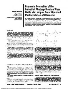
ometry would occur in a physiologically correct anastomosis 关17– 19兴. As a natural starting point, most of the numerical and in-vitro experiments have concentrated on geometries where the centerline of the bypass vessel and the centerline of the host vessel lie in a plane, as shown in Fig. 1共a兲, and may be termed planar. However, in this investigation we consider not only the flow in a planar model but also the effect of an out-of-plane distal anastomosis model where the centerline of the bypass vessel and the centerline of the host vessel no longer lie in a constant plane and may be termed nonplanar. There are many possible configurations for a nonplanar model depending on the local vascular geometry, for example the nonplanarity of the aortic bifurcation 关19兴, the use of vein cuffs 关20兴 or the introduction of a hood 关21兴. In the present study, we have restricted our attention to an anastomosis model where the bypass vessel is described by a torus that lies in a plane perpendicular to the original planar geometry, as shown in Fig. 1共b兲. For both geometries, the distal end-to-side anastomosis is modeled as a 45 deg junction, which is fully occluded upstream in a manner similar to the investigations of Steinman et al. 关13兴, Hofer et al. 关14兴, and Henry et al. 关15兴. The model geometries have been studied experimentally using magnetic resonance imaging 共MRI兲 and numerically using a computational fluid dynamics 共CFD兲 algorithm 关22兴. For our study, we have assumed that the model is noncompliant, that the flow is steady, and the fluid is Newtonian. The flow in arteries is clearly unsteady, the blood has non-Newtonian properties, and the walls are compliant. The local haemodynamics, however, as in any internal flow problem, are determined not only by these intrinsic properties of the flow but also by the boundary conditions at inflow, outflow, and on the wall, as induced by the local geometry. In modeling the flow in the large arteries 共with diameters of millimeters or above兲, it appears that the overall behavior is primarily affected by the basic geometry, the inflow and outflow conditions, and by the unsteadiness of the flow. Although the wall elasticity and non-Newtonian character of the fluid may be of considerable significance in, for example, transport mechanisms, several studies suggest they are of somewhat lesser importance as far as the gross features of the flow are concerned. Moore et al. 关23兴 compared MRI measurements of flow in the abdominal aorta in vivo and in a glass model 共designed to reproduce the three-dimensional in vivo anatomical geometry兲, and concluded that in vitro modeling could represent the major

Copyright © 2000 by ASME

Transactions of the ASME

Downloaded 26 Nov 2010 to 128.205.114.91. Redistribution subject to ASME license or copyright; see http://www.asme.org/terms/Terms_Use.cfm

A computer-controlled flow simulator 共Quest, Inc.兲 was used to provide the flow for the experiments. The circulating fluid used was a 60-40 by volume distilled water–glycerol solution. Its kinematic viscosity was measured with a capillary viscometer and was 3.416⫻10⫺6 m2/s at 20°C. For the planar model, a constant flow rate of 5.512 ml/s was applied corresponding to a Reynolds number of Re⫽250 based on the internal diameter of the pipe and the kinematic viscosity of the fluid used. 2.2

Fig. 1 Model geometries of distal end of the 45 deg end-toside anastomosis: „ a … planar, „ b … nonplanar

features of blood flow 共such as flow reversal and nonaxisymmetric profiles in the human aorta兲. Further discussion on the repercussions of assuming rigid walls and neglecting non-Newtonian effects to model in vivo flow is contained in the review of Friedman 关24兴. In sections 2.1 and 2.2, we review the experimental and numerical techniques employed and provide appropriate validation for each technique. In section 3.3 we show the comparison of the results of the MRI and CFD investigations within a planar geometry and discuss the salient features of this flow. Finally, in section 4.1, we discuss the significant flow characteristics in the planar and nonplanar models.

2

Materials and Methods 2.1

Experimental Technique

2.1.1 Model Construction. The planar anastomosis model was constructed using two Perspex pipes each of 8 mm internal diameter. The junction between the two pipes was milled to form a 45⫾1 deg junction and then the two pipes were adhered together. 2.1.2 Imaging. The MRI pulse sequence was of a twodimensional phase contrast type using a 1.5 Tesla ‘‘custom-built’’ small-bore scanner with 5.8 Gauss/cm gradient strength and a 300 ␮s rise time. The magnet was manufactured by Magnex 共UK兲 Ltd., the imaging electronics were built by GE Medical Systems 共Milwaukee, WI兲 and the RF coils and customized pulse sequences supplied by GE Research and Development Center 共Schenectady, NY兲. The field of view was 4 cm using a 256⫻256 image matrix, which produced a 0.156 mm/pixel resolution. A 30 deg flip angle was applied and a slice thickness of 2 mm was selected. The flow was encoded using a velocity encoding 共VENC兲 parameter of 22 cm/s for all velocity components. The VENC value was well above the highest measured velocities. Repetition time 共TR兲 for the scans was 33 ms and the echo time 共TE兲 or time between the center of the RF excitation pulses and the center of the echo was 17 ms. Given that data were extracted from a thin slice, 40 excitations 共NEX兲 were employed to compensate for the inherently low signal to noise ratio 共SNR兲 of the measurements. The acquisition took 22 minutes per slice location for all dimensions of flow encoding. Journal of Biomechanical Engineering

Computational Technique

2.2.1 Spectral/hp Algorithm. The computations were performed using a spectral/hp element algorithm 关22兴. In this technique the solution domain is decomposed into tetrahedral subdomains or elements as is typical of standard finite element or finite volume discretizations. However, unlike these standard techniques, each tetrahedral region is represented by a polynomial expansion. Convergence of the numerical solution may then be achieved by reducing the characteristic size of an element or increasing the order of the polynomial within each element. For smooth solutions, the advantage of a p-type approach is that high accuracy for a given amount of computational work can be obtained efficiently 关22兴. A further advantage of this method is that a refined simulation does not necessitate a redesign of the computational mesh, since a higher order polynomial expansion may be used within each tetrahedral element of the existing mesh. Finally, the complex curvature of the surface may also be accurately represented by the high-order polynomial expansion. The spectral/hp element method has been combined with a high-order splitting scheme 关25兴 to solve the time-dependent incompressible Navier–Stokes equations. The incompressible Navier–Stokes equations can be written as

⳵v ⫽⫺ⵜp⫹ ␯ L共 v兲 ⫹N共 v兲 ⳵t where L共 v兲 ⬅ⵜ 2 v N共 v兲 ⬅v•ⵜv⫽

1 ⵜ 共 v•v兲 ⫺v⫻ 共 ⵜ⫻v兲 , 2

and v and p denote the velocity vector and the pressure, respectively. The numerical splitting scheme can be written in three steps as J ⫺1

vˆ⫺vn e ⫽ ␤ q N共 vn⫺q 兲 ⌬t q⫽0

(1a)

v* ⫺vˆ ¯ n⫹1 ⫽⫺ⵜp ⌬t

(1b)

兺

J ⫺1

i vn⫹1 ⫺v* ␥ q L共 vn⫹1⫺q 兲 ⫽␯ ⌬t q⫽0

兺

(1c)

In the first step, 共1a兲, the nonlinear advection terms are advanced using either a convective or rotational form and are integrated in time using a multilevel Adams–Bashforth scheme denoted by the coefficients ␤ q . In the second step the time-averaged pressure ¯p is obtained by taking the divergence of 共1b兲, and assuming ⵜ•v*⫽0 to obtain a Poisson equation, which is supplemented with boundary conditions of the form

⳵ ¯p n⫹1 ⫽n• ⳵n

冋兺

J e ⫺1 q⫽0

J i ⫺1

␤ q N共 vn⫺q 兲 ⫺ ␯

兺

q⫽0

册

␤ q ⵜ⫻ 共 ⵜ⫻v兲 n⫺q .

These boundary conditions ensure that the splitting error associated with the scheme is consistent with the overall temporal discretization. Finally step 共1c兲 is re-arranged into a Helmholtz equation for each velocity component, which implies an implicit FEBRUARY 2000, Vol. 122 Õ 87


treatment of the viscous component using either an Euler backwards difference or Crank–Nicolson scheme, which are denoted by the coefficients ␥ q . 2.2.2 Computational Domains and Boundary Conditions. The computational domains for the planar and nonplanar geometries are shown in Fig. 1. For both meshes, the intersection of the centerline of the host and bypass vessels is located at the origin and the intersecting angle is taken to be 45 deg. In the planar geometry, shown in Fig. 1共a兲, the outflow was located 9 diameters 共D兲 downstream from the origin and the occlusion and inflow boundaries were located at 3D and 5D, respectively. The mesh contains 1742 elements with a viscous mesh region in the host artery of 0.1D thickness. In the nonplanar geometry, shown in Fig. 1共b兲, the outflow and occlusion were located at 10D and 3D from the origin, respectively. The nonplanar bypass vessel was decomposed into three sections: a region of straight pipe of length 1.5 connected to a 90 deg torus of radius 2D attached to another straight section pipe of length 1D. The torus was oriented so that its centerline lay in a plane perpendicular to the plane described by the intersection of the pipes’ centerlines. For this geometry 1946 elements were used with a viscous region of 0.1D thickness in the host artery. In both geometries, a Hagen–Poiseuille parabolic profile was imposed at inflow, which was suitably scaled to produce a unit mean velocity. All walls were treated as non-slip surfaces and the outflow was treated as a fully developed flow so that ⵜu•n⫽0, ⵜ v •n⫽0, ⵜw•n⫽0. The pressure at outflow was assumed to be constant. All computations were performed at three polynomial resolutions of order p⫽2, 4, and 6, which correspond to 17,420, 60,970, and 146,328 local degrees of freedom per variable in the planar case and 19,460, 68,110, and 163,464 in the nonplanar case. As mentioned previously, polynomial refinement is hierarchical and so all of the degrees of freedom used in the lower resolutions were contained within the higher resolution simulation. The solution was time marched until a steady-state solution was reached. It was assumed that the steady-state solution was achieved when the fluctuation in the force acting on the pipe as compared with the total force was smaller than 10⫺5 and a fluctuation of velocity in five history points was smaller than 10⫺5 when compared with the mean velocity. The history points were located at approximately ⫺5D, 0D, 1.5D, 2D, 3D along the centerline of the host vessel. Computational experiments on varying the length of the outflow boundary did not show any significant effect on the results within the region of interest. 2.2.3 Mesh Generation. The geometry of the model arteries is represented by means of CAD spline curves and surfaces to obtain a boundary representation 共B-Rep兲 of the computational domain. The B-Rep is then used as the analytical definition of the boundary to produce a discretization of the domain into a tetrahedral mesh. The mesh generation employs a modified advancing layers method for the near-wall regions 关26兴 and a method based on the advancing front technique 关27兴 for the rest of the domain. The resulting mesh of linear tetrahedra is finally transformed into a boundary conforming mesh of high-order elements. 2.2.4 Wall Shear Stress Calculation. A notable advantage of using a computational approach to simulate fluid flow is the ability to extract data on quantities that are extremely difficult, if not impossible, to determine experimentally. A flow quantity of particular interest in this investigation is the wall shear stress. The viscous stress ␶⫽ 关 ␶ 1 , ␶ 2 , ␶ 3 兴 T acting on an area of fluid with a normal n is defined as

冋

册

⳵ui ⳵u j ␶ i⫽ ␮ ⫹ n ⳵x j ⳵xi j where n⫽ 关 n 1 ,n 2 ,n 3 兴 T , v⫽ 关 u 1 ,u 2 ,u 3 兴 T , and ␮ is the coefficient 88 Õ Vol. 122, FEBRUARY 2000

of dynamic viscosity. Therefore the wall shear stress acting on an element of fluid at the wall ␶w can be determined using the wall normal nw . Although the wall shear stress here is expressed as a three-dimensional vector, it can be shown that this vector is orthogonal to the wall normal and therefore acts in a plane tangent to the wall. We may represent the wall shear stress in terms of a magnitude ␶ wss ⫽ 兩 ␶w 兩 and unit vector t⫽ ␶w / 兩 ␶w 兩 as ␶w ⫽ ␶ wss t.

3

Validation Results

3.1 Estimate of Experimental Uncertainty. Our uncertainty analysis of the experimental measurements identified that there was a precision error, due to random noise in the MRI measurements, of 10 percent at a 95 percent confidence level 共determined as the rms error as compared with the mean velocity兲. Initially a large systematic error was observed. This error was subsequently minimized by a recalibration of the MRI facility and a final systematic error of 2.5 percent with respect to the mean velocity was detectable. Therefore the uncertainty of the experimental process at a 95 percent confidence level, given by the root sum square of the bias and precision error, is 10.3 percent. These estimates were obtained by scanning a straight rigid 8 mm internal diameter tube model 共phantom兲 oriented along the axis of the magnet bore and under constant steady flow conditions. The MRI scanner and scan parameters were set to be the same as used in the model graft. Measurements were taken at different locations along the straight pipe and the experiment was repeated for a range of flow rates, which yielded Reynolds numbers between 250 and 600. Fully developed flow was ensured by only considering locations well beyond the entrance length 共L兲 which was estimated as L⫽0.03D Re, where Reynolds number is based on the pipe diameter D and mean flow velocity. The random and systematic errors were obtained by comparing the MRI profiles with the theoretical Hagen–Poiseuille flow profile. In order to avoid overestimation of the error levels due to the disproportionately high level of error in the near wall region, two pixels from each edge of the profile were discarded 共which is less than 6 percent of the total number of pixels in our experimental profiles兲. Having determined the experimental profile, a parabolic fit was put through the data using a least-squares approximation. The difference between the experimental data and this leastsquares fit was then taken to be the random measurement noise, while the difference between the experimental and theoretical parabolic profiles was used to determine the systematic error. An illustrative sample of the experimental axial flow profile across the pipe is shown in Fig. 2 at Re⫽390. Also shown is the leastsquares parabolic fit, which is coincident with the theoretical profile. 3.2 Numerical Accuracy. To determine the accuracy of the numerical computations we have used two indicators. The first measure uses the integral of the Cartesian pressure and viscous forces acting on all the walls of the models, which gives a single quantitative value. The second measure is the distribution of normalized wall shear stress in the vicinity of the bed of the anastomosis, which provides a field of information in a more qualitative measure. 3.2.1 Force Integrals. We define the force coefficients, C x , C y , C z , as C i⫽ 1 2

兩 F i兩

␳¯u 2 A

where F i is the integral of the pressure and shear forces over all walls in the ith direction, i.e., F i⫽

冕

共 pn i ⫹ ␶ i j n j 兲 ds,

walls



Table 1 Force coefficients C i Ä2 円 F i 円 Õ„ ␳ u¯ 2 A … acting on the walls of a planar model anastomosis, shown in Fig. 1„ a …, versus polynomial order at a mean Reynolds number of ReÄ250 Polynomial order (p) ⫺2

C x (⫻10 ) C y (⫻10⫺2 ) C z (⫻10⫺5 )

Fig. 2 Experimental measurement of the axial flow in a straight pipe at a Reynolds number of ReÄ390. Also shown is the least-squares fit to a parabolic profile, which is coincident with the theoretical parabolic solution at this Reynolds number.

␳ is the density, ¯u is the mean velocity and A is the surface area of the walls 共A⫽51.3 for the planar geometry兲. For a mean Reynolds ¯ D/␯⫽250 the value of the force coefficients at number Re⫽u steady state for different polynomial orders are shown in Table 1. From this table we see that the change in C x and C y between the simulations at p⫽2 and p⫽4 is 10.8 and 5.24 percent of the value at p⫽6; however, the difference between the simulations at p⫽4 and p⫽6 is only 0.4 and 1.5 percent, respectively. This variation demonstrates the level of ‘‘mesh convergence’’ in the solution and at p⫽6 is of the order of 1 percent in this flow variable. Finally we see from C z that the symmetry of the problem is recovered as we increase the polynomial order since C z is driven toward zero. 3.2.2 Normalized Wall Shear Stress. As discussed in section 2.2.4, the magnitude of wall shear stress ␶ wss is clearly dependent upon the first derivative of the velocity field v. In the spectral/hp element approach, as well as the finite element and finite volume methods, the velocity field is represented by a piecewise continuous polynomial approximation with C 0 continuity across elements. That is to say the numerical representation of v is continuous over the elemental boundaries but the derivative of v is not. Therefore, if the wall shear stress is approximated using the same numerical representation as the velocity field, then it will not be

2

4

6

3.623 7.549 0.310

4.054 7.965 4.078

3.992 7.934 1.416

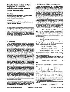
continuous over elemental boundaries unless the solution is completely resolved so the numerical solution closely approximates the exact smooth solution. Typically, CFD computations of the velocity field are postprocessed to recover a continuous approximation to the wall shear stress. However, this operation essentially smooths the wall shear stress. In the following computations we have calculated the wall shear stress using only the C 0 numerical polynomial representation of velocity and have not post-processed the results. Such an approach has been adopted since the jump in wall shear stress at elemental boundaries can be used as an indication of the resolution of the simulation. This point is illustrated in Fig. 3 where we see three plots of the numerical calculation of the magnitude of wall shear stress for the planar anastomosis model at Re⫽250 around the bed region. The plot has been normalized with the Hagen–Poiseuille wall shear stress at this Reynolds number. In the first plot, 3共a兲, the calculation was performed using a polynomial order of p⫽2 and the jumps in the wall shear stress magnitude directly correspond to the elemental boundaries of the computational mesh. In this calculation we have captured the general location of the maximum and minimum values, although the local shape of the features is not clear. In Fig. 3共b兲 a polynomial order of p⫽4 was used. The general continuity of the contours improves and the shape of the extreme values becomes better defined. Finally in Fig. 3共c兲, where a polynomial order of p⫽6 was applied, the majority of the contours are continuous and the shape of the maximum shear region is clear. The only noisy region is the region proximal to the heel. Here the flow is nearly stagnant, leading to a wall shear stress that is two orders of magnitude lower than the value at the peak. 3.3 Comparison of MRI and CFD Within the Planar Model. In this section we consider the steady flow in the planar anastomosis model using computational and experimental data, as previously studied by Steinman et al. 关13兴, with a view to validating the computational model and reviewing the flow within this configuration. Figure 4 shows the comparison of the axial component of velocity on three slices of the host vessel: one at 0.25D distal to the toe of the anastomosis, as defined in Fig. 1, and at 2D and 5D distal to the toe. The computational data have been

Fig. 3 Numerical calculation of the normalized wall shear stress in the planar anastomoses model around the bed region using a polynomial order of: „a… p Ä2, „b… p Ä4, „c… p Ä6. The same contour levels have been used in each plot.

Journal of Biomechanical Engineering

FEBRUARY 2000, Vol. 122 Õ 89


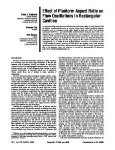
Fig. 4 Comparison CFD „top… and MRI „middle… axial velocity, normalized by flow rate per unit are, at „ a … 0.25D distal to the toe, „ b … 2 D distal to the toe, and „ c … 5 D distal to the toe. Also shown are a comparison of the CFD „dotted line… and MRI „solid line… profile of velocity extracted along the constant z centerline and normalized by mean velocity u¯ .

linearly averaged over five equally spaced slices of thickness 0.25D to take account of the slice thickness of the MRI data. All data have been normalized by the mean velocity, ¯u . The mean Reynolds number, based on the mean velocity, was 250 for both the MRI and the computational data. Also shown in Fig. 4 is the comparison of the CFD and MRI data through a horizontal section along the centerline of the data with error bars indicating the 10 percent experimental error. The flow should be interpreted as having a positive velocity as it moves into the page, toward the outflow of the domain. Figure 5 shows a comparison of the crossflow components 共v and w兲 captured using CFD and MRI at 0.3D distal to the toe of the graft. The agreement of the MRI and CFD data is generally good and within the experimental error. The plane of symmetry of the model about the centerline of the host and bypass vessel imposes a similar symmetry on the flow patterns as is illustrated by the cross sections in Figs. 4 and 5. We emphasize that this symmetry was not explicitly imposed in the computations. The velocity profiles in Fig. 4共a兲, at 0.25D, demonstrates that the parabolic axial flow pattern of the Hagen–Poiseuille flow has been translated toward the outer wall. The crossflow velocities shown in Fig. 5 are consistent with this translation. We note that the v -component is of the same order of magnitude as the axial u component. This strong crossflow component results from the pressure gradient introduced to balance the centrifugal force required to turn the flow. Thus the lower pressure at the toe of the graft drives a secondary flow pattern, as shown by the v -component velocity in Fig. 5共a兲. Associated with this secondary 90 Õ Vol. 122, FEBRUARY 2000

flow is a w-component velocity, which is necessarily symmetric about the horizontal centerline as shown in Fig. 5共b兲 and the combined motion of the v and w velocities is shown in the crossflow streamline plot shown in Fig. 5共c兲. Figure 4共b兲 shows the axial u component of velocity at 2D distal to the toe. The crescent form of this cross section, clearly captured in both the CFD and MRI results, is consistent with a Dean type flow, typically associated with flow within a torus 关28兴. Although it is not possible directly to identify the radius of curvature of the bypass pipe, it can be appreciated that the net effect of the bypass junction is to rotate the flow by 45 deg, which could have been achieved by a smooth transition in a curved pipe. Finally, Fig. 4共c兲 shows the axial u component of velocity at 5D distal to the toe. Although the crescent nature of the flow is still evident at this position, the viscous effects have started to play a greater role as the profile diffuses back to its steady-state parabolic profile, which would correspond to concentric circles in this figure. The rate of diffusion in the CFD and MRI results is similar. This should be expected as their respective Reynolds numbers are comparable. Finally we note that the agreement between the MRI and CFD velocity fields is not as good in the w component as in the other crossflow components shown in Fig. 5共b兲. This is due to the fact that the magnitude of velocities in this direction is noticeably smaller and, consequently, the experimental noise is more significant. Transactions of the ASME


Fig. 5 Comparison CFD „top… and MRI „bottom… crossflow data for the planar model at 0.25D distal to the toe: „ a … horizontal v component, „ b … vertical w component, „ c … crossflow streamlines. All data are normalized by the mean velocity u¯ .

4

Results and Discussion 4.1

Comparison of Planar and Nonplanar Geometries

4.1.1 Velocity Contours. Having considered the flow characteristics of the CFD and MRI results for the planar anastomosis model, which are generally in good agreement, we now compare the CFD results of the planar versus the nonplanar geometry. Figure 6 shows the axial u-component velocities normalized by ¯u at the toe, 2D and 5D distal to the toe for the planar and nonplanar model discussed in section 2.2.2. Both simulations were converged to a Reynolds number of Re⫽250 based on the mean velocity. The contours have been selected so that the planar and nonplanar cases are directly comparable at any given cross section. The nonplanar geometry exhibits a similar crescent forma-

tion typical of the Dean flow within a curved pipe. However, Fig. 6 shows that, in the nonplanar model, the crescent pattern is evident even at the toe in contrast to the planar model. Furthermore, the crescent has a bulk rotation as the flow moves distally and rotates in a clockwise sense as we look from the proximal toward the distal end of the host vessel. The motion is relatively pronounced having gone through a rotation of 180 deg in approximately five diameters. The sign of this rotation is consistent with the out-of-plane deformation of the bypass vessel where the bulk flow is pushed toward the outer radius of the torus section. We recall that for a curve that lies in a plane, the curvature is a measure of the variation of the curve from a straight line. For a more general curve at any point we can define a local plane of curvature 共using the local tangent and the derivative of the tangent

Fig. 6 Comparison of the CFD normalized axial velocity in planar „top… and nonplanar „bottom…: „ a … toe, „ b … 2 D distal to the toe, and „ c … 5 D distal to the toe




Fig. 7 Comparison of CFD computed normalized horizontal v -component crossflow velocity in planar „top… and nonplanar „bottom…: „ a … toe, „ b … 2 D distal to the toe, and „ c … 5 D distal to the toe

along the curve兲. As we move along this general curve, the plane of curvature will change and the torsion is a measure of the variation of this plane. A circle is a line of constant curvature but zero torsion and a helix is a line of constant curvature and torsion. Therefore, in the same way that the planar geometry might be idealized as a planar bend with an equivalent curvature, which generates the crescent shape of the axial flow, we could also envisage the nonplanar case as being represented by an equivalent helical shape, thereby introducing torsion into the problem. For steady flow within a helical pipe with sufficiently large curvature and torsion, an axial velocity profile of crescentic shape also develops similar to the planar bend 关29–31兴. However, in a helical pipe the crescent is not symmetric, which is also evident in the results of Fig. 6. Further, the numerical and experimental results from Doorly et al. 关32兴 have shown that when a helical pipe exits

into a straight pipe, a bulk rotation in the axial velocity is established due to the rotational inertia of the flow that develops within the helical pipe. Once again the role of viscosity is evident as the flow moves down the pipe, forcing the axial flow to return to its steady-state parabolic profile. Figures 7 and 8 show the comparison of the crossflow velocity components v and w, normalized by ¯u , for the planar and nonplanar models at the toe, at 2D and at 5D distal to the toe. In the planar model there are two recirculation regions, clearly marked by the three cells in the v -component velocity and the four cells in the w-component velocity. The intersection of the zero contours of the v and w velocity indicate the two points at which the flow is moving purely in the axial direction. These points can be considered as the crossflow stagnation points or the equivalent location of a line vortex in the flow, which is oriented along the

Fig. 8 Comparison of CFD normalized computed vertical w -component crossflow velocity in planar „top… and nonplanar „bottom…: „ a … toe, „ b … 2 D distal to the toe, and „ c … 5 D distal to the toe

92 Õ Vol. 122, FEBRUARY 2000



cal level, the dominance of one recirculation region is to be expected, since the nonplanarity causes a nonsymmetric injection of the flow into the host artery, with the centroid of the velocity being displaced below the horizontal plane of symmetry of the host artery.

Fig. 9 Comparison of the normalized axial velocity at the heel of the anastomosis for: „ a … planar, „ b … nonplanar geometries

x-direction. From the contours of v -component velocity in the planar geometry shown in Fig. 7 we see that these points move from their location near the outer wall at the toe toward the center of the vessel as the upper and lower cells grow in magnitude. Figure 8 shows a slight motion of the stagnation points from left to right as the flow moves distally from the toe. This slight motion is illustrated by the contour of zero w-velocity in the planar model at the toe, which is located slightly to the left of the center. However, by 2D distal to the toe, the contour has moved to the right of the centerline, and by 5D the contour has established a more central doubly symmetric location. In contrast, the crossflow within the nonplanar model demonstrates a noticeably different structure. As is to be expected, there is no longer a plane of symmetry, and although there are initially two recirculation regions, as indicated by the three cells in v -velocity and four cells in w-velocity, the bottom recirculation region is weak. As we move distally from the toe, the top and bottom cells in the v -component velocity of Fig. 7 grow under the action of diffusion and bring the crossflow stagnation point toward the center of the cross section. The bottom cell, however, is clearly weaker and at the 5D section is almost indiscernible. It can be noticed, from the w-component velocities in the nonplanar model of Fig. 8, that there is a transition from two to one recirculation cells. Initially at the toe, we see four cells indicating two recirculation regions. As the flow progresses distally, at the 2D section, the top left and bottom right cells have started to coalesce, causing the bottom left cell to become increasingly smaller. Finally at 5D the existence of two w-component cells indicates that only one recirculation region is present. As noted in Zabielski and Mestel 关31兴, a single recirculation cell is a particular feature of nonplanar flows due to torsion. The occurrence of a single cell is typically found at low Dean numbers, which are associated with a large radius of curvature, as is clearly the case in the straight section of the host vessel after the anastomosis. On a more physi-

4.1.2 Flux of Flow at Heel. After considering the flow development as we move distally from the anastomosis, we now analyze the proximal region to the anastomosis within the host vessel. In a fully occluded vessel there is a stagnant region proximal to the anastomosis. Such a region may be physiologically undesirable due to the potential development of intimal hyperplasia at the heel. We would therefore like to consider the role of the nonplanar geometry in the flow characteristics at this region. Figure 9 shows the axial u-component of velocity, normalized by ¯u , in the cross-plane located at the heel for the planar and nonplanar models. Using the same convention as in previous plots, flow moving toward the outflow is represented by a negative contour. Positive contours indicates flow entering the occluded region proximal to the anastomosis. The bypass vessel is located on the right-hand side of the cross sections and therefore the negative contours indicate an entrainment of flow into the junction. This flux of flow out of the occluded region is replaced by a positive flux located near the bed, as shown on the left hand side of the section. Since there is no other source of flow entering this region, the net flux of flow across the plane is necessarily zero. However, the magnitude of the contours provide an indication of the amount of fluid recirculating within this region. In both the planar and nonplanar models, the magnitude of axial velocity is relatively ¯ ⭐0.047 in the small, having a value in the interval ⫺0.065⭐u/u ¯ ⭐0.097 in planar model and a value in the interval ⫺0.101⭐u/u the nonplanar model, as compared with a peak velocity of 2 at the inflow. However, the introduction of nonplanarity has almost doubled the peak of axial velocities crossing this section. The large velocities do not necessarily indicate an integrated effect of flow across the whole section and, perhaps, the average integrated absolute velocity over the cross section, i.e., 兩u兩⫽

兰兩 u 兩 ds ␲r2

where r is the pipe radius is a better measure. For the planar ¯ ⫽1.93⫻10⫺2 and for the nonplanar model we find that 兩 u 兩 /u ¯ model we find that 兩 u 兩 /u ⫽3.51⫻10⫺2 where ¯u is the mean flow. Although this represents an 80 percent increase the absolute flux only rises from 1.93 to 3.5 percent of the mean flow, which is still comparatively small.

Fig. 10 Comparison of CFD computed wall shear stress normalized by the steady straight pipe wall shear stress for: „ a … planar, „ b … nonplanar geometries




Fig. 11 Comparison of CFD pressure coefficients along the wall for: „ a … planar, „ b … nonplanar geometries

4.1.3 Wall Forces. The final part of the investigation of the role of out-of-plane geometry considers the direct and tangential stresses on the host vessel in the region of the anastomosis. Figure 10 shows a map of the magnitude of wall shear stress ␶ wss for the two models. These values have been normalized with respect to the wall shear stress of the Hagen–Poiseuille flow within a straight pipe of the same diameter. The map should be interpreted so that the horizontal axis represents distance along the axis of the host vessel and the vertical axis represents the circumferential distance along the wall of the host vessel. The map has been chosen so that the bed region appears at the center. For the planar geometry shown in Fig. 1共a兲 the symmetry of the flow is once more evident, reaching a peak value of 3.72 in the region of the bed just distal to the toe. The circular region of low stress just adjacent to this peak can be attributed to the stagnation point, while the low flow rate at the heel seen in Fig. 9 is clearly associated with a region of low wall shear stress. As mentioned previously, the wall shear stress has been calculated directly from the velocity field and so the numerical wall shear stress might not be continuous across element boundaries. The overall continuous appearance of the wall shear stress is an indication of the resolved nature of the computation. However, there is some evidence of jumps in the wall shear stress in the low wall shear stress region proximal to the anastomosis. The wall shear stress in this region is about two orders of magnitude smaller than the peak shear stress at the bed, which is consistent with the level of numerical error at a polynomial order of p⫽6 as discussed in section 2.2.2. In Fig. 10共b兲 we see the nonplanar geometry distribution using the same contours as shown in Fig. 10共a兲. We note that for the nonplanar model the region of peak shear at the bed of the junction has been reduced to a peak value of 3.37, which is approximately 10 percent lower than that of the planar model. Although there is only a 10 percent reduction in the peak value, the contours of the maximum around this peak have been noticeably altered as indicated by the absence of contour levels at 3.4 and 3.6. The region of maximum wall shear stress at the bed has also extended proximally, as compared with the planar model, reducing the extent of the low shear region around the stagnation point. Further, the contours of low wall shear stress to the right of the heel decrease at a slower rate consistent with the increase of flow recirculating in the nonplanar model, as compared with the planar case. For completeness, Fig. 11 shows the pressure coefficient along the wall of the host vessel in the region of the bed of the anastomosis. The pressure coefficient is defined as ¯ p⫺p C p⫽ 1 u2 2 ␳¯ 94 Õ Vol. 122, FEBRUARY 2000

where ¯p denotes the average pressure at the outflow location of the planar model; ␳ is the density and ¯u is the mean velocity. From this figure we can conclude that the reduction in peak wall shear stress in the nonplanar simulation is associated with an increase in the peak pressure coefficient relative to the pressure coefficient at 9D distal to the junction. As discussed previously, there is clearly a negative pressure gradient in the circumferential direction from the bed toward the toe.

5

Summary

The comparison between the MRI measurements and the CFD simulations within a 45 deg planar model anastomosis at Re⫽250 has been used to validate the computational technique and gain understanding of the steady Newtonian flow characteristics. The inherent symmetry of this flow model has been removed by considering an out-of-plane deformation of the bypass vessel. The role of introducing this three dimensionality can be viewed in terms of a helical-type motion of the flow as it moves from the bypass to the host vessel as compared to an idealization of a curvature induced transition in the planar model. Considering the planar model in terms of a curvature induced motion explains the occurrence of a crescent shape in the axial flow component associated with crossflow velocity established as the flow is turned through 45 deg. However, when considering the helical motion of a nonplanar anastomosis, model torsion as well as curvature effects are present. The introduction of torsion breaks the symmetry of the planar model and we see evidence of a single recirculation region developing in the crossflow velocity components as the flow moves distally, compared to the existence of two recirculation regions in the planar model. Further, the nonplanar model reduces the peak in the wall shear stress magnitude by 10 percent at the bed of the anastomosis as compared with the planar model and introduces an 80 percent increase in absolute flux of velocity into the occluded region proximal to the anastomosis. Nevertheless the absolute flux of velocity into the occluded region is still comparatively small being only 3.5 percent of the mean flow. A simple modification of the geometry of an end-to-side anastomosis, whereby the graft is rendered approximately helical, has been shown to profoundly affect the flow field and can also be expected to influence the particle residence times. In view of the reported association between the flow field and vascular biology, the development of intimal hyperplasia, and atherosclerosis, the results may have pathophysiological implications in relation to geometry. Current investigations are now focused on the role of pulsatility within the context of planar and nonplanar geometries of end-to-side anastomosis. Transactions of the ASME


Acknowledgments The authors would like to acknowledge the Department of Health and the generous support provided by the General Electric Company 共USA兲 for funding of the MRI experiments. We would also like to acknowledge Garfield Weston Foundation for partial support. O. Shah is supported by the EPSRC and Harefield Advanced Technology under a CASE award. The computations were performed on the Imperial College Parallel Computing facility Fujitsu AP3000 and the Biomedical Visualisation Origin 2000 system.

关15兴关16兴

关17兴关18兴

References 关1兴 Bryan, A., and Angelini, G., 1994, ‘‘The Biology of Saphenous Vein Graft Occlusion: Etiology and Strategies for Prevention,’’ Curr. Opin. Cardiol., 9, pp. 641–649. 关2兴 Davies, P., 1995, ‘‘Flow Mediated Endothelial Mechanotransduction,’’ Physiol. Rev., 75, pp. 519–560. 关3兴 McIntire, L., 1997, ‘‘Differential Gene Regulation Induced by Flow in Vascular Cells: Implications for Gene Therapy,’’ in: Proc. International Conference on New Frontiers in Biomechanical Engineering, Bioengineering Division, JSME. 关4兴 Ojha, M., Ethier, C., Johnston, K., and Cobbold, R., 1990, ‘‘Steady and Pulsatile Flow Fields in an End-to-Side Arterial Anastomosis Model,’’ J. Vasc. Surg., 20, pp. 311–317. 关5兴 Sottiuari, V., Yao, J., Batson, R., Sue, S., Jones, R., and Nakamura, Y., 1989, ‘‘Distal Anastomotic Intimal Hyperplasia: Hystopathologic Character and Biogenesis,’’ Ann. Vasc. Surg., 29, pp. 26–33. 关6兴 Bassiouny, H., White, S., Glagov, S., Choi, E., Giddens, D., and Zarins, C., 1992, ‘‘Anastomotic Intimal Hyperplasia: Mechanical Injury or Flow Induced,’’ J. Vasc. Surg., 15, pp. 708–717. 关7兴 Ojha, M., 1993, ‘‘Spatial and Temporal Variations of Wall Shear Stress Within an End-to-Side Arterial Anastomosis Model,’’ J. Biomech., 114, No. 12, pp. 1377–1388. 关8兴 Lei, M., Kleinstreuer, C., and Archie, J., 1997, ‘‘Haemodynamic Simulation and Computer-Aided Designs of Graft-Artery Junctions,’’ ASME J. Biomech. Eng., 119, pp. 343–348. 关9兴 Ku, D., and Giddens, D., 1983, ‘‘Pulsatile Flow in a Model Carotid Bifurcation,’’ Atherosclerosis, 3, pp. 31–39. 关10兴 Friedman, M., Bargeron, C., Deters, O., Hutchins, G., and Mark, F., 1987, ‘‘Correlation Between Wall Shear and Intimal Thickness at a Coronary Artery Branch,’’ Atherosclerosis, 68, pp. 27–33. 关11兴 Yamamoto, T., Tanaka, H., Jones, C. J. H., Lever, M., Parker, K. H., Kimura, A., Hiramatsu, O., Ogasawara, Y., Tsujioka, K., Caro, C. G., and Kajiya, F., 1992, ‘‘Blood Velocity Profiles in the Origin of the Canine Renal Artery and Their Relevance in the Localization and Development of Atherosclerosis,’’ Arterioscler. Thromb., 12, No. 5, pp. 626–632. 关12兴 Asakura, T., and Karino, T., 1990, ‘‘Flow Patterns and Spatial Distribution of Atherosclerotic Lesions in Human Coronary Arteries,’’ Circ. Res., 66, pp. 1045–1066. 关13兴 Steinman, D., Frayne, R., Zhang, X.-D., Butt, B., and Ethier, C., 1996, ‘‘MR Measurements and Numerical Simulation of Steady Flow in an End-to-Side Anastomosis Model,’’ J. Biomech., 29, No. 4, pp. 537–542. 关14兴 Hofer, M., Rappitsch, G., Perktold, K., Trubel, W., and Schima, H., 1996,


关19兴关20兴关21兴

关22兴关23兴关24兴关25兴关26兴关27兴关28兴关29兴关30兴关31兴关32兴

‘‘Numerical Study of Wall Mechanics and Fluid Dynamics in End-to-Side Anastomoses and Correlation to Initimal Hyperplasia,’’ J. Biomech., 29, pp. 1297–1308. Henry, F., Collins, M., Hughes, P., and How, T., 1996, ‘‘Numerical Investigation of Steady Flow in Proximal and Distal End-to-Side Anastomoses,’’ ASME J. Biomech. Eng., 118, pp. 302–310. White, S., Zarins, C., Giddens, D., Bassiouny, H., Loth, F., Jones, S., and Glagov, S., 1993, ‘‘Hemodynamics Patterns in Two Models of End-to-Side Vascular Graft Anastomoses: Effects of Pulsatility, Flow Division, Reynolds Number and Hood Length,’’ ASME J. Biomech. Eng., 114, pp. 104–115. Caro, C., Doorly, D., Tarnawski, M., Scott, K., Long, Q., and Dumoulin, C., 1996, ‘‘Non-Planar Curvature and Branching of Arteries and Non-Planar-Type Flow,’’ Proc. R. Soc. London, Ser. A, 452, pp. 185–197. Sherwin, S., Shah, O., Doorly, D., Mclean, M., Watkins, N., Caro, C., Peiro, J., Tarnawski, M., and Dumoulin, C., 1997, ‘‘Visualisation and Computational Study of Flow in Model Planar and Non-planar End-to-Side Arterial Bypass Grafts,’’ Physiological Society Abstracts, Plymouth. Ding, Z., and Friedman, M., 1997, ‘‘Variability in Planarity of the Aortic Bifurcation Measured From Magnetic Resonance Images,’’ in: Bioengineering Conference, ASME BED-Vol. 35. DaSilva, A., Carpenter, T., How, T., and Harris, P., 1997, ‘‘Stable Vortices Within Vein Cuffs Inhibit Anastomotic Myointimal Hyperplasia?’’ Eur. J. Vasc. Endovasc Surg., 14, No. 3, pp. 157–163. Loth, F., Jones, S., Giddens, D., Bassiouny, H., Glagov, S., and Zarins, C., 1997, ‘‘Measurement of Velocity and Wall Shear Stress Inside a PTFE Vascular Graft Model Under Steady Flow Conditions,’’ ASME J. Biomech. Eng., 119, No. 2, pp. 187–195. Sherwin, S., and Karniadakis, G., 1996, ‘‘Tetrahedral hp Finite Elements: Algorithms and Flow Simulations,’’ J. Comp. Physiol., 124, pp. 14–45. Moore, J. E., Maiser, S., Ku, D., and Bo¨siger, P., 1994, ‘‘Haemodynamics in the Abdominal Aorta: a Comparison of In-Vitro and In-Vivo Measurements,’’ J. Appl. Physiol., 76, pp. 1520–1527. Friedman, M. H., 1993, ‘‘Arteriosclerosis Research Using Vascular Flow Models: From 2-D Branches to Compliant Replicas,’’ ASME J. Biomech. Eng., 115, No. 4, pp. 595–601. Karniadakis, G., Israeli, M., and Orszag, S., 1991, ‘‘High-Order Splitting Methods for the Incompressible Navier–Stokes Equations,’’ J. Comp. Physiol., 97, pp. 414–443. Peiro, J., and Sayma, A. I., 1995, ‘‘A 3-D Unstructured Multigrid Navier– Stokes Solver,’’ in: K. W. Morton and M. J. Baines, eds., Numerical Methods for Fluid Dynamics, V, Oxford University Press. Peraire, J., Peiro, J., and Morgan, K., 1993, ‘‘Multigrid Solution of the 3-D Compressible Euler Equations on Unstructured Tetrahedral Grids,’’ Int. J. Numer. Methods Eng., 36, pp. 1029–1044. Dean, W., 1928, ‘‘The Streamline Motion of Fluid in a Curved Pipe,’’ Philos. Mag., 5, pp. 673–695. Tuttle, E., 1990, ‘‘Laminar Flow in Twisted Pipes’’ J. Fluid Mech., 219, pp. 545–570. Kao, H., 1987, ‘‘Torsion Effects on Fully Developed Flow in a Helical Pipe,’’ J. Fluid Mech., 184, pp. 335–356. Zabielski, L., and Mestel, A., 1998, ‘‘Steady Flow in a Helically Symmetric Pipe,’’ J. Fluid Mech., 370, pp. 297–320. Doorly, D., Peiro, J., Sherwin, S., Shah, O., Caro, C., Tarnawski, M., Maclean, M., Dumoulin, C., and Axel, L., 1997, ‘‘Helix and Model Graft Flows: MRI Measurements and CFD Simulations,’’ Proc. ASME FED Meeting, ASME Paper No. FEDSM-97-3423.



Using ASME format - iacm-forth

Using ASME format - iacm-forth

Suggest Documents