Dec 21, 2012 ... ... or the training site http://download.eiva.dk/online-training/NaviPac.htm .... Refer
to the manual on timing principles. •. You may type a more ...
NAVIPAC INTRODUCTION & WORKFLOW
Author: Ole Kristensen Last update: 21/12/2012 Version: 3.9
Contents
Page 2 of 12
1
Introduction to NaviPac ................................................................................................. 3
2
Program Environment .................................................................................................... 4
3
HW Environment ............................................................................................................. 7
4
Workflow example .......................................................................................................... 8
1 Introduction to NaviPac In this document the various components in the NaviPac SW will be briefly described. Also a simple workflow of using the SW is included. Finally an example of a HW configuration is outlined. The NaviPac navigation software consists of several sub-parts, but from a user’s point of view it can be divided into 2 main parts: The Configuration Scenario and the Online Scenario. Use the Configuration program to define the geodesy and instrument set-up. The Online part of the system collects various sensor data and calculates a final filtered position a/o.
For further details please refer to the EIVA home page www.eiva.dk or the training site http://download.eiva.dk/online-training/NaviPac.htm
2_Introduction to NaviPac.docx Last update: 21/12/2012
Page 3 of 12
2 Program Environment Below the NaviPac software environment is outlined.
Figure 1 NaviPac software Environment In the figure the system is described as 5 primary blocks. The NaviPac Config program does not depend on the other programs. This means that it can be run stand-alone. Everything that the user set-up by the program is stored in the Gensetup.DB (a binary database file that holds all set-up) and an ASCII file called NAVIPAC.INI.
Page 4 of 12
The Kernel represents a series of background processes that handles interfacing, calculations and distribution
The Data I/O program reads data from the connected instruments connected to the serial ports. E.g. data from GPS, Gyro, Speed Log... The QC/Kernel programs calculate the final position based on the selected LOPs by filtering data from the sensors and also calculate a predicted position - used in next calculation. The Data Distributor periodically reads data from the QC/Kernel and distributes it to running GUI processes that have requested data to be displayed. E.g. position, gyro in the Online main window, QC information in the QC window(s), position data to Helmsman etc.
The Data I/O, QC/Kernel, Data Distributor and the Online program can be started from the Set-up program. They will read information required from the Set-up DB (database). In fact the Set-up database consists of 2 parts:
a static part created by the Set-up program a more dynamic part where current LOP selection etc. are stored (Online database). The last one will be named Online DB. E.g. Data I/O read the port settings for the instruments, Online/Kernel reads LOP (Line Of Position) information etc.
The Online program handles the entire navigation operation, i.e. selection of LOPs, collection of sensor data, computation of positions, presentation of data, calibration, adjustment of navigation attributes etc. This program can be executed (displayed) on more computers at the same time. The dynamic information of LOPs included etc. are stored in a system file named Online DB. Only the online program can modify it and the QC/Kernel will use it heavily. The Online database will include the following information: Information
Includes
Selected LOPs
Definition of the selected LOPs including LOP type, name and all needed parameters.
Selected Additional Instruments
Definition of selected (if any) instruments for dead reckoning (gyro and speed log) if any.
Selected objects for dynamic
Definition of objects and systems selected for UW or remote positioning.
positioning LOP control parameters
Various parameters used for LOP control (C-O, weight, sigma, filters, priorities etc.).
Fixed offsets
Information about the user defined offsets in action
Estimated Position
Last known position for estimation.
Navigation Mode
Last used navigation mode.
Time Control
Defines how the NaviPac time is controlled (GPS, PC, ...)
2_Introduction to NaviPac.docx Last update: 21/12/2012
Page 5 of 12
Table 1 Information stored in the Online database
The Config program handles definition of the global and static system parameters, and will in most cases be inactive during most of the operational time. The program is typical limited to the master computer at the time, but it may if needed be started on any computer - i.e. last user who saves overwrites previous user’s set-up. The NaviPac Config program saves information in a system file (Setup database). The system set-up includes all static background information needed throughout operation and may even include additional non-used information. There will not be any need for change in this set-up, unless basic information is changed. The Set-up database will include the following information: Information
Includes
Selected Projection
Definition of the selected projection (e.g. UTM-32) including projection type, projection name and various projection parameters.
Selected Ellipsoid
Definition of the selected ellipsoid (e.g. International 1924) including ellipsoid type, ellipsoid name and various ellipsoid parameters.
Defined Datum shift
Definition of the defined datum shift (between WGS 84 and user datum) including all 7 parameters.
ITRF
Is ITRF enables – and the given base parameters
Included Surface Navigation
List of all included surface navigation systems (e.g. Ashtech GPS, Motorola mini-
Systems
ranger, Racal Microfix etc.) identified by system type and system name and if needed additional system parameters.
Available Stations
List of available stations (system definitions) for each surface navigation system. Station name, station location, station parameters and availability flag give each station.
Defined Instruments
List of included instruments given by type (e.g. Surface Navigation), instrument (Ashtech GPS), layback offsets, I/O mode (On, Off, Simulated or Calculated) and I/O set-up.
Additional Instrument
For each instrument in the above list, this part includes additional parameters if
Parameters
needed.
Data Scale
Selected position and depth unit – eg. Metric or US Survey Feet
Table 2 Information stored in the Set-up database
Page 6 of 12
3 HW Environment Below an example of the NaviPac HW environment is outlined.
Figure 2 - Example of NaviPac HW/network configuration
There are no limits on the number of computers that NaviPac can be installed on. The only requirements are that:
TCP/IP network protocol is installed on all computers. Windows XPP or higher. NaviPac is installed with a dongle on the master PC (Server) – all other computers are NaviPac “slaves” (clients) that do no interfacing but present different functions (like Helmsman’s display) to the users. Beside network connections dual video boards can be used to present more “screen” space to the applications. Video splitters are another alternative.
2_Introduction to NaviPac.docx Last update: 21/12/2012
Page 7 of 12
4 Workflow example A typical workflow using the NaviPac programs will be difficult to describe as it depends on the task that should be solved. But in this chapter we assume that the user wants to create a new Set-up database with some basic instruments defined before the NaviPac Online system is started. The steps to go through to set-up the NaviPac system would be:
Page 8 of 12
Start the configuration program If Online is running it can be started from the File menu Otherwise use the Windows NaviPac program group. The current general set-up database will automatically be loaded If you want to create a new database from basic Activate File, New Activate File, Save As Save the file to \eiva\navipac\db\gensetup.db Set-up Projections & Ellipsoids Expand the Geodesy section Select Projection Right mouse click and select Edit Settings Perform the setup and accept by OK Set-up Datum Shift Expand the Geodesy section Select Datum Shift Right mouse click and select Edit Settings Perform the setup and accept by OK Set-up Working Unit Expand the Geodesy section Select Scale Right mouse click and select Edit Settings Perform the setup and accept by OK DEFINE INSTRUMENTS FOR THE VESSEL Expand the Object section Select the first item in the list (default named Vessel) At the right part of the window (the property control) select the Name filed and type the vessel name – accept by ENTER ADD GPS Expand the Instruments section Select Surface Navigation Activate right mouse and select Add New Item Select the sensor you want to add and accept by OK Select the correct interfacing setup
Type the offsets from CRP to sensor (X across vessel + starboard, Y along vessel + front, Z plus up) Accept by OK The instrument is added to the list and selected. Sensor details are shown at the right part. If you are using a ellipsoid different from WGS84 and have defined a datum shift then please make sure to select Apply Datum Shift Please consider carefully how time tagging of the sensor is performed – eg. Refer to the manual on timing principles You may type a more reasonable name for the instruments as this helps identifying the right sensor at a later stage ADD GYRO Expand the Instruments section Select Gyro Activate right mouse and select Add New Item Select the sensor you want to add and accept by OK Select the correct interfacing setup Type the offsets from CRP to sensor (X across vessel + starboard, Y along vessel + front, Z plus up) Accept by OK The instrument is added to the list and selected. Sensor details are shown at the right part. You may enter a sensor C-O (value that will be added to the observed data) to compensate for mounting misalignments Please consider carefully how time tagging of the sensor is performed – eg. Refer to the manual on timing principles You may type a more reasonable name for the instruments as this helps identifying the right sensor at a later stage ADD MOTION SENSOR Expand the Instruments section Select Motion Sensor Activate right mouse and select Add New Item Select the sensor you want to add and accept by OK Select the correct interfacing setup Type the offsets from CRP to sensor (X across vessel + starboard, Y along vessel + front, Z plus up) Accept by OK The instrument is added to the list and selected. Sensor details are shown at the right part. You may enter a C-O for roll, pitch and heave (value that will be added to the observed data) to compensate for mounting misalignments Please consider carefully how time tagging of the sensor is performed – eg. Refer to the manual on timing principles You may type a more reasonable name for the instruments as this helps identifying the right sensor at a later stage
2_Introduction to NaviPac.docx Last update: 21/12/2012
Page 9 of 12
Page 10 of 12
ADD ECHOSOUNDER Expand the Instruments section Select data Acquisition Activate right mouse and select Add New Item Select the sensor you want to add and accept by OK Select the correct interfacing setup Type the offsets from CRP to sensor (X across vessel + starboard, Y along vessel + front, Z plus up) Accept by OK The instrument is added to the list and selected. Sensor details are shown at the right part. You may enter a sensor timeout value defining how long time NaviPac must wait on data before triggering an alarm. Please consider carefully how time tagging of the sensor is performed – eg. Refer to the manual on timing principles You may type a more reasonable name for the instruments as this helps identifying the right sensor at a later stage For each channel on the acquisition sensor (up to 3 – eg. DESO 25 may have 3) the channels are shown below the sensor Select the cannel Type a reasonable name Click Active Enter offsets (if there) DEFINE INSTRUMENTS FOR A ROV via USBL Expand the Objects section Right click at Objects and select Add New Item A second object is added to the list Select the item in the list and change the name to eg MY-ROV ADD POSITION FOR THE ROV Expand the Instruments section Select Dynamic Positioning Activate right mouse and select Add New Item Select the sensor (eg. HPR 410/HiPAP)you want to add and accept by OK Select the correct interfacing setup Type the offsets from CRP to sensor reference point (X across vessel + starboard, Y along vessel + front, Z plus up) Accept by OK The instrument is added to the list and selected. Sensor details are shown at the right part. For USBL data please make sure to enter correct settings for USBL Hold Time (5 seconds or more) and USBL mountings Please consider carefully how time tagging of the sensor is performed – eg. Refer to the manual on timing principles You may type a more reasonable name for the instruments as this helps identifying the right sensor at a later stage
Select the instrument in the list and activate right mouse and select Add object An entry is added below the instrument. Select it and check the right side Select the ROV name Enter a TP code corresponding to the settings in the USBL system You may now add instruments (Gyro, Motions Sensor, Data Acquisition and DVL) to the ROV as done for the vessel earlier. Just remember to select the correct Location Finally “Save” the current defined set-up by selecting File, Save. This will create a Set-up database (file: $EIVAHOME/DB/gensetup.DB).
In the following it is assumed that the user has created a Set-up database as described above and the user wants to start from scratch - e.g. no navigation system is running. The steps to go through for the Online navigation would be:
Start the Online program From NPConfig press the Start navigation button. If this for some reason fails expand the File Header entry and select DB version – right mouse and select Manual Start. A dialogue pops up enabling the user to select the positioning systems that are wanted during the navigation session. It is also possible to select if the ROV should be positioned or not (i.e. moved from Available to Included. Note: this functionality can also be used when the system is started.) When OK is selected a new dialogue appears allowing the user to specify an estimated position of the ship - the last one entered will be shown. When done select OK and the background processes will be started (DataIO, Kernel, etc.). If physical sensors are connected an estimated position will be updated each second in the Online main window. If alarm condition a red colour will be used as background colour in the status field. If all instruments are simulated you have to type a speed and gyro value in the Simulator window to simulate a move of the ship and thereby get updated positions. The next possible task for the navigator will depend on the situation. If alarms occur (red state and alarm messages presented in message list) a typical task could be to start up Base Positions and watch the different LOPs data. Watch the error- and std. deviation values in Base Positions and find out which navigation system is the error source. The low quality LOP’s are normally weighted down automatically. Compare eventually with other groups reference positions and they give “better” data change navigation mode or the reference priority group number. Navigation mode can be set to Auto Prioritised Positioning in the Navigation Mode menu item in the Navigation menu. The priority groups and reference group can be changed by selecting the Navigation, Navigation Mode, Change Priority menu in the Online main window.
2_Introduction to NaviPac.docx Last update: 21/12/2012
Page 11 of 12
Page 12 of 12
Also watch the QC (Quality Control) data for the LOPs. This can be started from the View, QC menu. A detailed graphical view with error ellipse and std. deviation can be displayed for each of the up to 5 navigation groups (note: if navigation mode is “Auto Multi Positioning” only one button (prio 1) is shown.) If some of the connected sensors seem to give “unusable” data the raw data from the sensors can be studied on the port by selecting View, Raw Data. This wills startup a program where the ports can be selected one by one and you can see if the data is as expected.