Optimized Space Vector Pulse-width Modulation Technique for a Five ...

Journal of Power Electronics, Vol. 14, No. 5, pp. 937-945, September 2014

937

http://dx.doi.org/10.6113/JPE.2014.14.5.937 ISSN(Print): 1598-2092 / ISSN(Online): 2093-4718

JPE 14-5-15

Optimized Space Vector Pulse-width Modulation Technique for a Five-level Cascaded H-Bridge Inverter Amarendra Matsa†, Irfan Ahmed*, and Madhuri A. Chaudhari* †*

Department of Electrical Engineering,Visvesvaraya National Institute of Technology, Nagpur, India

Abstract This paper presents an optimized space vector pulse-width modulation (OSVPWM) technique for a five-level cascaded H-bridge (CHB) inverter. The space vector diagram of the five-level CHB inverter is optimized by resolving it into inner and outer two-level space vector hexagons. Unlike conventional space vector topology, the proposed technique significantly reduces the involved computational time and efforts without compromising the performance of the five-level CHB inverter. A further optimized (FOSVPWM) technique is also presented in this paper, which significantly reduces the complexity and computational efforts. The developed techniques are verified through MATLAB/SIMULINK. Results are compared with sinusoidal pulse-width modulation (SPWM) to prove the validity of the proposed technique. The proposed simulation system is realized by using an XC3S400 field-programmable gate array from Xilinx, Inc. The experiment results are then presented for verification. Key words: Five-level cascaded H-bridge inverter, Optimized SVPWM, Power electronics, Space vector pulse-width modulation (SVPWM)

I.

-

INTRODUCTION

The need for a high-power control apparatus has developed in various industrial applications in recent years. Thus, several multilevel converter structures have been introduced as alternatives to high-power and medium-voltage applications. Multilevel converters not only achieve high-power ratings but also achieve the integration of distributed generation (DG) sources. Multilevel converters have three principal topologies [1], [2].Among which, the cascaded H-bridge (CHB) topology is the most suitable for DG sources [3].Pulse-width modulation (PWM) techniques for multilevel converters have been studied extensively during the last few decades. A wide variety of methods, which are different in concepts and performances, have been developed to achieve one or more of the following objectives: wide linear modulation range less switching losses decreased total harmonic distortion(THD) Manuscript received May 15, 2014; accepted Jun. 20, 2014 Recommended for publication by Associate Editor Rae-Young Kim. † CorrespondingAuthor:[email protected] Tel:+91-9492904858,Visvesvaraya National Institute of Technology * Dept. of Electrical Eng., Visvesvaraya Nat’l Institute of Tech., India

easy implementation and less computational time [4], [5]. The space vector pulse with modulation (SVPWM) technique provides superior harmonics capacity and solves the problem of unbalanced capacitor voltages by using redundant states in the space voltage vector plane. Thus, many methods have been developed to implement SVPWM to drive voltage-source inverters [2]-[16].SVPWM implementation generally involves identifying sectors, determining switching vectors, and selecting optimum switching sequences for inverters [6], [7]. Blasko provided a classical SVPWM technique with an equal duration of zero-state vector V0 application, whereas V7 was modified. A factor-variable Ko that is proportional to the time of application of vector V7 was introduced. By changing Ko from zero to one, the duration of V7application can be changed from 0% to 100% of the combined application time for zero-state vectors. A correlation between the modified space-vector and triangle-comparison methods (with added zero sequence) was established[8].Celanovic introduced a new and computationally efficient space vector modulation (SVM) algorithm for general n-level converters. This algorithm can be implemented on nearly any commercially available digital signal processor and is suited for execution in real time;

© 2014 KIPE

938

Journal of Power Electronics, Vol. 14, No. 5, September 2014

(a) N2 P2 N2

N1 P2 N2

N1 P2 N1 N2 P1 N2

N2 P2 N1

N1 P2 O N2 P1 N1

N2 P2 O

N1P 2P 2 N2P 1P 1

N2P 2P 2

N2OP 2

OP1 P2 N1OP 1 N2N 1O

N1OP 2 N2N1 P1

N2 N2P 2

P1P 2O OP1 N1 N1ON 2

P2 P2 N2

P 2P 2N1 P 1P 1N2

P2 P2 O P1 P1 N1 OON 2 P2 P2 P1 P1 P1 O OON 1 N1 N1 N2

P 2P 1 N2

P 2P 1N1 P 1ON2 P2P 1O P1ON 1 ON1 N2

P 2ON2

P 2ON1 P 1N1 N2

P 2N1 N2

P2 P2 P2 P 2P1 P1 P2OO P1 P1 P1 P 2 N1 N1 P 1OO P 2N2 N2 P1N 1N1 OOO ON 1 N1 ON2 N2 P 1 N2 N2 N1 N1 N1 N 1N2 N2 N2 N2 N2 P1P1 P2 P2 P1 P2 P2 OP1 P 2N1 O OOP1 P1 OP1 P1 N1 O P2 N2N1 N1N1 O ON 1O P 1N2 N1 ON2 N1 N2N2 N1 N1 N2 N1

OOP 2 N1 N1 P1 N2 N2 O

N1 N1P 2 N2 N2P 1

N2 N1P 2

P 1P 2N1 OP 1N2

P 1P2 P1 OP 1 O N 1ON 1 N 2N1 N2 P1P2 P2 OP1 P1 N1OO N2N1 N1

OP 2P2 N1 P1 P1 N2 OO

N1P 1P 2 N2OP 1

N2 P1 P2

OP 2N1 N1 P1 N2

OP2 O N1 P1 N1 N2 ON2

OP 2 P1 N 1P1 O N 2ON 1

N1 P2 P1 N2P1 O

N2 P2 P1

P 1P 2 N2

OP 2 N2

P1OP 2 ON1 P1 N1N 2O

ON1 P2 N1 N2P 1

N1 N2P 2

P2 OP2 P1 N1 P1 ON2 O

P 1N1 P2 ON2 P1

ON2P 2

P1 N2P 2

P 2N1 P1 P 1N2 O P2 N1P 2 P1 N2P 1

P 2N2O

P 2N2 P1

P2 N2P 2

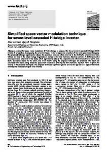
(b) Fig. 1. (a) Five-level CHB inverter.(b) SVD of a five-level inverter.

however, this method is more complex than others[9].Seo proposed a simplified SVPWM method for a three-level inverter. This method is based on the simplification of the space vector diagram (SVD) of a three-level inverter into that of a two-level inverter [10].Perales developed a 3D space vector algorithm for a multilevel converter to compensate for the harmonics and zero-sequence components of the system. This algorithm is useful in systems with or without neutrality, unbalanced load, and triple harmonics, as well as for generating 3D control vectors[11].Ahmed also developed a new simplified SVPWM technique for a seven-level inverter. This technique can reduce the complexity of an SVD [12]. The schematic structure of a five-level CHB inverter is shown in Fig. 1(a) and its SVD is shown in Fig.1(b). This inverter has five possible output voltage levels for each phase. The levels, which range from +2E (corresponding to P2) to −2E (corresponding to N2), result in 53 = 125 possible space

vectors for the inverter. The number of independent space vectors is(3n2−3n+1) = 61, where n = 5 for the five levels. (n − 1) = 4 layers and (n − 1)3 = 64 triangles are found in the SVD. This paper proposes an optimized technique for SVPWM (OSVPWM) of a five-level CHB multilevel inverter. This technique considerably reduces calculation time, complexity, and efforts involved in constructing the SVD of a five-level CHB inverter. Based on the geometric simplification of the SVD, the proposed method reduces the number of two–level hexagons that should be considered from 36 to 24 (18 outer + 6 inner) for a five-level inverter. A further OSVPWM (FOSVPWM) technique is also proposed in this paper which further reduces the number of two-level hexagons to 18.The simulation results of both techniques for a five-level CHB inverter are presented and compared with the results of the sinusoidal PWM technique (SPWM) to validate the proposed methods.

939

Optimized Space Vector Pulse-width Modulation Technique for…

II.

PROPOSED OSVPWM TECHNIQUE

The basic idea of OSVPWM is based on the concept of resolving a five-level SVD[Fig. 1(b)] into inner and outer two-level hexagons. The selectivity of the inner and outer regions depends on the magnitude of Vref. If Vref magnitude is less than 2E, then the inner region is selected; otherwise, the outer region is selected as shown in Fig. 2. The hexagons in the outer or inner region are selected based on the angle θ of the original reference voltage. When Vref is more than 2E, the outer region hexagons are selected. Selecting a particular hexagon in the outer region depends on angle θ as shown in Table I. When an outer hexagon is selected, a new reference vectorVrefo2 is generated, such that it originates from the center of the outer two-level hexagons. The tip of this new vector coincides with the tip of Vref5.Consider the case of hexagon I(OH1) shown in Fig.3.Vector Vrefo2 is related to Vref5based on the following relations: Vo2α = V5α – 3E, (1) Vo2β= V5β, (2) where V5α,V5β and Vo2α,Vo2β are the components of Vref5and Vrefo2along the real and imaginary axes, respectively. The mapping of all Vrefo2hexagons is described in Table II. Vector Vrefo2 for each of the outer hexagons has a modulation index ranging from zero to unity and an angle θo2 ranging from zero to 2π. Angle θo2 is also applied to each of the outer hexagons. When the inner two-level hexagons (IH) are selected, reference vector Vref5 is mapped to the inner two-level hexagon center reference vector Vrefi2 as shown in Fig. 4. The appropriate selection of IH depends on angle θ5. The process of selecting an appropriate inner two-level hexagon is described in Table III. Consider the case of selecting an inner two-level hexagon1 (IH1) as shown in Fig. 5. Reference vectors Vrefi2 and Vref5 are related as follows:

Vi2α = V5α – E, (3) Vi2β = V5β, (4) where V5α,V5β and Vi2α,Vi2β are the components of Vref5 and Vrefi2 along the α and β axes, respectively. The computation Vrefi2 of all six inner two-level hexagons is described in Table 4.

III. DWELL TIME CALCULATION AND SWITCHING SEQUENCE DESIGN Dwell time calculation and switching sequence generation for the selected two-level hexagon can be performed in a manner similar to that in the conventional two-level SVPWM technique. Each two-level hexagon is divided into six sectors. The sector in reference vector Vrefo2 depends on its angle θo2.Vrefo2 can then be synthesized by the three stationary vectors of that sector. Dwell time calculation for the stationary vectors is performed based on the “volt-second-balancing” principle. The outer region two-level

TABLEI SELECTION OF OUTER TWO-LEVEL HEXAGONS Range of θ Hexagon number −15°to +15° OH1 +15°to +30° OH2 +30°to +45° OH3 +45°to +75° OH4 +75°to +90° OH5 +90°to +105° OH6 +105° to +135° OH7 +135°to +150° OH8 +150° to +165° OH9 +165°to −165° OH10 −165°to −150° OH11 −150° to −135° OH12 −135°to −105° OH13 −105° to −90° OH14 −90°to −75° OH15 −75° to −45° OH16 −45°to −30° OH17 −30° to −15° OH18

hexagon OH1and reference voltage Vrefo2 lie in Sector I as shown in Fig.5. VectorsV1 (P2N2N2),V2 (P2N1N2) and P2N1N1,P2N2N2 are zero voltage vectorsV0. The volt-second-balancing equation for this sector is given as follows: Vrefo2Ts= V1Ta+ V2Tb+ V0T0, (5) where Ts is the sampling interval; and Ta, Tb, andT0 are the respective dwell times for vectors V1, V2, and V0. The values of Ta, Tb, and T0 are given as follows: Π

Ta = Ts×ma Sin ( − θ),

(6)

Tb = Ts×maSin θ, To = Ts – Ta−Tb,

(7) (8)



where ma is the modulation index defined as follows: Vref

(9) √3  . After calculating dwell time intervals, an appropriate design for the switching sequence is required. The typical seven-segment switching sequence is used in this scheme. The switching sequence should be designed, such that a change from one switching state to the next involves only one leg, and a change from one sector to the next involves zero or a minimum number of switching [1]. With these constraints, the seven-segment switching sequence for vector Vrefo2 Sector I shown in Fig.5 is given as follows: (P1N2N2),(P2N2N2),(P2N1N2),(P2N1N1),(P2N1N2), (P2N2N2), (P1N2N2). Similarly, the switching sequence for Sector II is given as follows: (P1N2N2), (P2N2N2), (P2N1N2), (P2N1N1), (P2N1N2), (P2N2N2), (P1N2N2). Ma=

940

Journal of Power Electronics, Vol. 14, No. 5, September 2014

Fig. 2. Selection of inner and outer regions.

Hexagon number OH1

TABLE II MAPPING OFVREFO2FROM VREF5 VO2α V5α – 3E 

VO2β V5β 

OH2

V5α – 2.598076211E cos

V5β− 2.598076211E sin

OH3

V5β− 2.598076211E sin

V5β− 2.598076211E sin

OH4

V5α – 3 E cos

OH5

V5α – 2.598076211E cos

V5β− 2.598076211E sin

OH6

V5α– 2.598076211E cos

V5β− 2.598076211E sin

OH7

V5α – 3E cos

OH8

V5α – 2.598076211E cos

V5β− 2.598076211E sin

OH9

V5α – 2.598076211E cos

V5β− 2.598076211E sin

OH10

  



  



V5β−3E sin

 

  



    



V5β− 3E sin

    

V5α + 3 E

    

V5β 



OH11

V5α – 2.598076211E cos

V5β− 2.598076211E sin

OH12

V5α – 2.598076211E cos

V5β− 2.598076211E sin

OH13

V5α – 3E cos

OH14

V5α – 2.598076211E cos

V5β − 2.598076211E sin

OH15

V5α – 2.598076211E cos

V5β− 2.598076211E sin

OH16

V5α – 3E cos

OH17

V5α – 2.598076211E cos

V5β− 2.598076211E sin

OH18

V5α – 2.598076211E cos

V5β− 2.598076211E sin

  



  



V5β− 3E sin

    



 

  



V5β− 3E sin

    

    

941

Optimized Space Vector Pulse-width Modulation Technique for…

OH7

OH6

OH5

OH4

OH3

OH 1

Vref5

OH2

Inner region

Vrefo2

Θ4

OH1

TABLE III SELECTION OF INNER TWO-LEVEL HEXAGONS Range of θ Hexagon number −30°to +30° IH1 +30°to +90° IH2 +90° to +150° IH3 +150° to −150° IH4 −150°to −90° IH5 −90°to −30° IH6

Θ o2

TABLE IV MAPPING OFVREFI2FROM VREF5

3E OH 18

OH 17

Fig. 3. Outer two-level hexagon reference point mapping.

Hexagon IH1 IH2

Vi2α V5α – E  V5α – E cos

Vi2β V5β  V5β−E sin

IH3 IH4 IH5

V5α – E cos  V5α + E  V5α – E cos

V5β−E sin  V5β  V5β −E sin

IH6

V5α – E cos

V5β −E sin

 

  

 

  

TABLE V SELECTION OF THE OUTER TWO-LEVEL HEXAGONS IN THE FOSVPWM TECHNIQUE Range of θ Hexagon number +0° to +30° OH2 +30° to +60° OH3 +60° to +90° OH5 +90° to +120° OH6 +120° to +150° OH8 +150° to +180° OH9 −180°to −150° OH11 −150° to −120° OH12 −120° to −90° OH14 −90° to −60° OH15 −60°to −30° OH17 −30°to −0° OH18 Fig. 4. Inner two-level hexagon reference point mapping.

IV.

Fig. 5. Outer region two-level hexagon OH1.

FOSVPWM

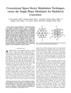
This technique further reduces the number of two-level hexagons that should be considered. Consequently, it decreases the complexity and efforts involved in the SVPWM of a five-level inverter. A five-level SVD for this technique is initially resolved into inner and outer regions, similar to in the OSVPWM technique. Thus, the number of two-level hexagons that should be considered for the FOSVPWM of a five-level inverter is reduced to 18. The modulation index Ma for SVM is defined as the maximum value(Ma = 1) that corresponds to the radius of the largest circle that can be inscribed in the SVD. The five-level SVD with such a circle is shown in Fig. 6. If only 12 OHs are considered (even for Ma = 1), then only the dark shaded portion of the SVD is left unattended. If this area is ignored, then the SVM of a five-level inverter involves only 18 two-level hexagons. Selecting the appropriate two-level hexagon depends on the magnitude and

942

Output line voltage(Vab)

Journal of Power Electronics, Vol. 14, No. 5, September 2014

2000 1000 0 -1000 -2000 0

0.01

0.02

0.03

0.04

0.05

0.06

0.07

0.08

TABLE VI SIMULATION PARAMETERS USED FOR FIVE-LEVEL CHB INVERTER H-bridge DC supply voltage E = 600 V System frequency f = 50 Hz Three-phase resistive load (star) RL = 100 Ω

angle of reference vector Vref5 described in Table V. The decrease in complexity is achieved at the cost of a slightly increased THD of the output voltage. This increase is only for Ma> 0.75, where Ma is the modulation index for the five-level SVD. If the tip of vector Vref5 lies in the dark unattended portion, then one of the OHs is selected depending on the angle θ5 of Vref5. A new reference vector Vrefo2 is then generated, as in the case of the OSVPWM technique, with its origin located at the center of the selected two-level hexagon.

V.

SIMULATION RESULTS

The proposed methods are simulated with MATLAB/SIMULINK. The simulation is conducted for a five-level CHB inverter at different values of the modulation index Ma. The results are compared with those of the conventional SPWM technique to validate the viability of the proposed techniques. The simulation parameters are shown in Table VI, and the simulation results are shown in Figs.7 and 8 for the modulation indices Ma= 1.0 and Ma=0.8, respectively. The sampling frequency for the SVM schemes is generally preferred as 6N times the output frequency, where N is an integer. The sampling frequency for the SVM schemes is fs = 1.5 kHz, assuming a value of N = 5. For the SPWM schemes, the sampling frequency should be [(2N + 1) × 3] times the output frequency [17], [18]. Thus, fs = 1.65 kHz for these

2000 1000 0 -1000 -2000 0

0.01

0.02

0.03

0.04

0.05

0.06

0.07

0.08

0.04

0.05

0.06

0.07

0.08

Time(s)

Output line voltage(Vab)

Fig. 6. Five-level SVD with an inscribing circle for Ma = 1.

Output line voltage(Vab)

Time(s)

2000 1000 0 -1000 -2000 0

0.01

0.02

0.03

Time(s)

Fig. 7. Output line voltage waveforms at Ma = 1 for SPWM, OSVPWM and FOSVPWM. (b) OSVPWM. (c) FOSVPWM. TABLE VII THD AND PEAK VALUE OF FUNDAMENTAL COMPONENT (V1M) OF OUTPUT LINE VOLTAGE Modulation SPWM OSVM FOSPWM Technique Ma = 1.0 THD,% 17.12 20.67 21.55 V1m, V 2106 2348 2265 Ma =0.8 THD, % 21.71 22.99 24.09 V1m, V 1708 2216 2172 Ma= 0.6 THD, % 25.61 29.2 29.2 V1m, V 1321 1824.6 1824.6 Ma= 0.4 THD, % 42.15 38.58 38.58 V1m, V 1184.3 1688 1688 Ma = 0.2 THD, % 91.87 49.96 49.96 V1m, V 718 1326 1326

schemes. Table VII shows the THD of the output line voltage and the peak magnitude of the fundamental components at various Ma values.

Optimized Space Vector Pulse-width Modulation Technique for…

943

Output line voltage(Vab)

2000 1000 0 -1000

-2000 0

0.01

0.02

0.03

0.04

0.05

0.06

0.07

0.08

0.05

0.06

0.07

0.08

(a) OSVPWM.

Output line voltag(Vab)

Time(s)

2000 1000 0 -1000 -2000 0

0.01

0.02

0.03

0.04

Output line voltage(Vab)

Time(s)

(b) FOSVPWM. Fig. 10. Output line voltage waveforms at Ma = 1 for OSVPWM and FOSVPWM.

2000 1000 0 -1000 -2000 0

0.01

0.02

0.03

0.04

0.05

0.06

0.07

0.08

Fig. 8. Output line voltage waveforms at Ma = 0.8 for SPWM, OSVPWM and FOSVPWM. (a) SPWM. (b) OSVPWM. (c) FOSVPWM. Time(s)

(a) OSVPWM.

(b) FOSVPWM. Fig. 11. Output line voltage waveforms at Ma = 0.8 for OSVPWM and FOSVPWM.

Fig. 9. Experimental setup of Five- level H-Bridge Inverter.

TABLE VIII EXPERIMENTAL PARAMETERS USED FOR FIVE-LEVEL CHB INVERTER H-bridge DC supply voltage E = 200 V System frequency f = 50 Hz Three-phase resistive load (star) RL = 1.5KW

944

Journal of Power Electronics, Vol. 14, No. 5, September 2014

These results show that the proposed optimized techniques are comparable with the established SPWM schemes. The proposed techniques exhibit satisfactory performance for all values of the modulation index Ma. The THD obtained with these techniques is slightly higher than that obtained with the SPWM scheme. In addition, the fundamental components of the output voltage obtained with these schemes are higher than those obtained with the SPWM scheme. The proposed schemes also exhibit significant improvement over the SPWM scheme for low values of Ma. In particular, for Ma ≤ 0.2, the FOSVPWM scheme presents remarkable improvement in performance over the SPWM scheme. This condition is advantageous in applications wherein the inverter may sometimes be required to operate at low modulation indices. Thus, the proposed techniques perform comparably with the previously proposed SVM techniques for multilevel inverters while considerably optimizing the control algorithm.

VI.

EXPERIMENT RESULTS

An experimental study was conducted to confirm the proposed control methods. Experimental set up as shown in Fig.9, in which two H-bridges are connected in series per phase. An XC3S400 field-programmable gate array (FPGA) from Xilinx, Inc. (California, USA) was used to realize the proposed control schemes. The experimental system parameters are listed in Table VIII.

VII.

CONCLUSIONS

This study presents the OSVPWM technique that optimizes the SVPWM of multilevel inverters. The proposed technique is based on resolving the multilevel inverter SVD into inner and outer region two-level hexagons. This technique is general and can be applied to the SVPWM of all three principal topologies for multilevel converters at any number of levels. The advantage of applying this technique increases as the number of levels increases. An FOSVPWM technique has also been presented for the SVM of a five-level inverter. This technique reduces the complexity and effort required for the SVPWM of a five-level inverter by nearly 50%. In particular, the OSVPWM technique reduces the five-level SVPWM to a SVPWM problem of 24 two-level hexagons. The FOSVPWM technique further reduces this number to 18. The simulation results for both techniques are presented for a five-level CHB inverter. The results are compared with those of the SPWM technique, which proves the validity of the proposed techniques for different values of the modulation index. The experiment results are then provided for the proposed methods to verify the correctness of the real-time simulation system. The FPGA-based real-time

emulation will be a popular component of real-time simulation. The application of these techniques significantly reduces the complexity and efforts involved in the SVPWM of higher level inverters.

REFERENCES [1] B. Wu, High-Power Converters and AC Drives, John Wiley & Sons, Chap. 7, 2006. [2] J. Rodriguez, J. Lai, and F. Z. Peng, “Multilevel inverters: a survey of topologies, controls, and applications,” IEEE Trans. Ind. Electron., Vol.4 9, No. 4, pp. 724-738, Aug. 2002. [3] E. Pouresmaeil, O. Gomis-Bellmunt, D. Montesinos-Miracle, and J. Bergas-Jane, “Multilevel converters control for renewable energy integration to the power grid,” Energy, Vol. 36, No. 2, pp. 950-963, Feb. 2011. [4] J. Holtz, “Pulse-width-modulation–A survey,” IEEE Trans. Ind. Electron., Vol. 39, No. 5, pp. 410-419, Dec.1992. [5] S. R. Bowesand and Y. S. Lai, “The relations hip between space-vector modulation and regular-sampled PWM,” IEEE Trans. Ind. Electronics,Vol. 44, No. 5 pp. 670-679, Oct. 1997. [6] S. K. Mondal, J. P. Pinto, and B. K. Bose, “A neural network- based space vector PWM controller for a three level voltage-fed inverter induction motor drive,” IEEE Trans. Ind. Electron., Vol. 38, No. 3, pp. 660-669, May/Jun. 2002. [7] M. M. Renge and H. M. Suryawanshi, “Five-level diode clamped inverter to eliminate common mode voltage and reduce dv/dt in medium voltage rating induction motor drives,” IEEE Trans. Ind. Electron., Vol. 23, No. 4, pp. 1598-1607, Jul.2008. [8] V. Blasko, “Analysis of a hybrid PWM based on modifiedspace-vector and triangle-comparison methods,” IEEE Trans.Ind.Appl., Vol. 33, No. 3, pp. 756-764, May/Jun. 1997. [9] N. Celanovic and D. Boroyevich, “A fast space-vector modulation algorithm for multilevel three-phase converters,” IEEE Trans. Ind. Appl., Vol. 37, No. 2, pp. 637-641, Mar./Apr. 2001. [10] J. H. Seo, C. H. Cho, and D. S. Hyun, “A new simplified space-vector PWM Method for three-level Inverters,” IEEE Trans.Power Electron., Vol. 16, No. 4, pp. 545-550, Jul. 2001. [11] M. M. Prats, L. G. Franquelo, R. Portillo, J. I. León, E. Galván, and J. M. Carrasco, “A 3-D space vector modulation generalized algorithm for multilevel converters,” IEEE Power Electronics Letters, Vol. 1, No. 4, pp. 110-114, Dec. 2003. [12] I. Ahmed and V. B. Borghate, “Simplified space vector modulation technique for seven-level cascaded H-bridge inverter,” IET Power Electron., Vol. 7, No. 5, pp. 604-613, Mar. 2014. [13] S. Wei, B. Wu, F. Li, and C. Liu, “A general space vector PWM control algorithm for multilevel inverters,” in Proc. 18th Annual IEEE APEC, Vol. 1, pp. 562-568, 2003. [14] A. S. A. Mohamed, A. Gopinath, and M. R. Baiju, “A simple space vector PWM generation scheme for any general n-level inverter,” IEEE Trans. Ind. Electron., Vol. 56, No. 5, pp. 1649-1656, May 2009.

Optimized Space Vector Pulse-width Modulation Technique for…

945

[15] D. Lalili, N. Lourci, E. M. Berkouk, F. Boudjema, J. Petzoldt, and M. Y. Dali, “A simplified space vector pulse width modulation algorithm for fivelevel diode clamping inverter,” in Proc. SPEEDAM, pp. 1349-1354, 2006. [16] R. Rabinovici, D. Baimel, J. Tomasik, and A. Zuckerberger, “Series space vector modulation for multi-level cascaded H-bridge inverters,” IETPower Electron., Vol. 3, No. 6, pp. 843-857, Mar.2010. [17] J. A. Houldsworth, and D. A. Grant, “The use of harmonic distortion to increase the output voltage of a three-phase PWM inverter,” IEEE Trans. Ind. Electron., Vol. 20, No. 5, pp. 1224-1228, Oct.1984.

Irfan Ahmed received his B.E. (Electrical Engineering) from Nagpur University, India, in 2001, and M.Tech (Power Electronics, machines, and drives) from the Indian Institute of Technology, Roorkee, India, in 2004. From 2004 to 2011, he worked as a faculty member at Anjuman College of Engineering and Technology, Nagpur, India. He is currently pursuing his Ph.D. at the Department of Electrical and Electronics Engineering, VNIT, Nagpur, India. His research interests include power electronics and its applications to power systems and drives

Amarendra Matsa was born in Andhra Pradesh, India on August 23, 1984. He received his B.Tech and M.Tech degrees from Jawaharlal Nehru Technological University, Hyderabad, India in 2006 and 2009, respectively. He is currently pursuing his Ph.D. at Visvesvaraya National Institute of Technology (VNIT), Nagpur, India. His current research interests include power electronics, new control algorithm techniques for grid-integrated distributed generation, and microgrids.

Madhuri A. Chaudhari was born in Maharashtra, India on January 28, 1968. She received her B.E. from Amaravati University, Amaravati, India; M.Tech from Visvesvaraya Regional College of Engineering, Nagpur University, Nagpur, India; and Ph.D. from VNIT, Nagpur, India (all in electrical engineering). She is currently an associate professor at the Department of Electrical Engineering, VNIT. Her research interests are in the areas of power electronics, FACTS, and AC–DC drives. Dr. Chaudhari is a member of the IEEE, the Institution of Engineers (India), and the Indian Society for Technical Education.