Using ASME format

Transactions Journal of of the ASME Dynamic Systems, ®

Dynamic Systems and Control Division Technical Editor, A. GALIP ULSOY Past Editors, W. BOOK M. TOMIZUKA D. M. AUSLANDER J. L. SHEARER K. N. REID Y. TAKAHASHI M. J. RABINS Associate Technical Editors, Y. CHAIT „2002… F. CONRAD „2001… E. FAHRENTHOLD „2001… S. FASSOIS „2001… Y. HURMUZLU „2001… R. LANGARI „2002… E. MISAWA „2002… S. NAIR „2001… N. OLGAC „2001… C. RAHN „2002… S. SIVASHANKAR „2002… J. TU „2002… P. VOULGARIS „2001…

Measurement, and Control Published Quarterly by The American Society of Mechanical Engineers

VOLUME 122 • NUMBER 1 • MARCH 2000

TECHNICAL PAPERS 1

Block Control Principle for Mechanical Systems Vadim I. Utkin, De-Shiou Chen, and Hao-Chi Chang

11

Passivity and Noncollocation in the Control of Flexible Multibody Systems Christopher J. Damaren

18

Fast Control of Linear Systems Subject to Input Constraints P. Tomas Larsson and A. Galip Ulsoy

27

A Simplified Cartesian-Computed Torque Controller for Highly Geared Systems and Its Application to an Experimental Climbing Robot David Bevly, Steven Dubowsky, and Constantinos Mavroidis

33

Control of a Class of Mechanical Systems With Uncertainties Via a Constructive AdaptiveÕSecond Order VSC Approach A. Ferrara and L. Giacomini

OFFICERS OF THE ASME Chairman, R. E. NICKELL Executive Director D. L. BELDEN Treasurer J. A. MASON

40

A Repetitive Learning Method Based on Sliding Mode for Robot Control T. S. Liu and W. S. Lee

49

Disturbance Rejection With Simultaneous Input-Output Linearization and Decoupling Via Restricted State Feedback A. S. Tsirikos and K. G. Arvanitis

PUBLISHING STAFF Managing Director, Engineering CHARLES W. BEARDSLEY Director, Technical Publishing PHILIP DI VIETRO Managing Editor, Technical Publishing CYNTHIA B. CLARK Managing Editor, Transactions CORNELIA MONAHAN Production Assistant MARISOL ANDINO

63

Robust Input Shaper Control Design for Parameter Variations in Flexible Structures Lucy Y. Pao and Mark A. Lau

71

Distributed-Parameter Modeling for Geometry Control of Manufacturing Processes With Material Deposition Charalabos Doumanidis and Eleni Skordeli

78

Modeling and Identification of Lubricated Polymer Friction Dynamics Geesern Hsu, Andrew E. Yagle, Kenneth C. Ludema, and Joel A. Levitt

89

Fractal Estimation of Flank Wear in Turning Satish T. S. Bukkapatnam, Soundar R. T. Kumara, and Akhlesh Lakhtakia

95

Experimental Identification of Dynamic Parameters of Rolling Element Bearings in Machine Tools D. M. Shamine, S. W. Hong, and Y. C. Shin

102

Error Analysis of the Cylindrical Capacitive Sensor for Active Magnetic Bearing Spindles Hyeong-Joon Ahn, Soo Jeon, and Dong-Chul Han

108

Robust Stabilization of Large Amplitude Ship Rolling in Beam Seas Shyh-Leh Chen, Steven W. Shaw, Hassan K. Khalil, and Armin W. Troesch

114

A Sliding Mode Control of a Full-Car Electrorheological Suspension System Via Hardware in-the-Loop Simulation S. B. Choi, Y. T. Choi, and D. W. Park

Book Review Editor A. GALIP ULSOY Executive Committee Chairman, G. MASADA Past Chairman, N. NATHOO Vice Chairman, C. RADCLIFFE Members, J. STEIN S. JAYASURIYA Secretary, C. DESILVA BOARD ON COMMUNICATIONS Chairman and Vice-President R. K. SHAH

Transactions of the ASME, Journal of Dynamic Systems, Measurement, and Control (ISSN 0022-0434) is published quarterly (Mar., June, Sept., Dec.) for $215.00 per year by The American Society of Mechanical Engineers, Three Park Avenue, New York, NY 10016. Periodicals postage paid at New York, NY and additional mailing offices. POSTMASTER: Send address changes to Transactions of the ASME, Journal of Dynamic Systems, Measurement, and Control, c/o THE AMERICAN SOCIETY OF MECHANICAL ENGINEERS, 22 Law Drive, Box 2300, Fairfield, NJ 07007-2300. CHANGES OF ADDRESS must be received at Society headquarters seven weeks before they are to be effective. Please send old label and new address. PRICES: To members, $40.00, annually: to nonmembers, $215.00. Add $40.00 for postage to countries outside the United States and Canada. STATEMENT from By-Laws. The Society shall not be responsible for statements or opinions advanced in papers or ... printed in its publications (B7.1, Para. 3). COPYRIGHT © 2000 by The American Society of Mechanical Engineers. Authorization to photocopy material for internal or personal use under those circumstances not falling within the fair use provisions of the Copyright Act, contact the Copyright Clearance Center (CCC), 222 Rosewood Drive, Danvers, MA 01923, tel: 978-750-8400, www.copyright.com. Request for special permission or bulk copying should be addressed to Reprints/Permission Department. Reprints from this publication may be made on condition that full credit be given the TRANSACTIONS OF THE ASME, JOURNAL OF DYNAMIC SYSTEMS, MEASUREMENT, AND CONTROL, and the author, and date of publication be stated. INDEXED by Applied Mechanics Reviews and Engineering Information, Inc. Canadian Goods & Services Tax Registration #126148048.

„Contents continued on inside back cover…

„Contents continued… Journal of Dynamic Systems, Measurement, and Control

MARCH 2000

Volume 122, Number 1 122

Control-Oriented Model for Camless Intake Process—Part I M.-S. S. Ashhab, A. G. Stefanopoulou, J. A. Cook, and M. B. Levin

131

Control of Camless Intake Process—Part II M.-S. S. Ashhab, A. G. Stefanopoulou, J. A. Cook, and M. B. Levin

140

Control of Deep-Hysteresis Aeroengine Compressors Hsin-Hsiung Wang, Miroslav Krstic´, and Michael Larsen

153

Fluid Transmission Line Modeling Using a Variational Method Jari Ma¨kinen, Robert Piche´, and Asko Ellman

163

Nonlinearity and Feedback Compensation Method in a Pneumatic Vibration Generator B. Kuzńiewski

168

Theoretical and Experimental Investigations of an Opto-Pneumatic Detector G. Belforte, T. Raparelli, V. Viktorov, G. Eula, and A. Ivanov

174

Instantaneous Flow Rate Measurement of Ideal Gases Kenji Kawashima, Toshiharu Kagawa, and Toshinori Fujita

179

A Linearized Electrohydraulic Servovalve Model for Valve Dynamics Sensitivity Analysis and Control System Design Dean H. Kim and Tsu-Chin Tsao

188

Adaptive Control With Asymptotic Tracking Performance and Its Application to an Electro-Hydraulic Servo System Zongxuan Sun and Tsu-Chin Tsao

196

Robust Speed Control of a Variable-Displacement Hydraulic Motor Considering Saturation Nonlinearity Chul Soo Kim and Chung Oh Lee

202

Position Control of a Cylinder Using a Hydraulic Bridge Circuit With ER Valves Seung-Bok Choi and Woo-Yeon Choi

210

Modeling of Digital-Displacement Pump-Motors and Their Application as Hydraulic Drives for Nonuniform Loads Md. Ehsan, W. H. S. Rampen, and S. H. Salter

216

Tipping the Cylinder Block of an Axial-Piston Swash-Plate Type Hydrostatic Machine Noah D. Manring

TECHNICAL BRIEFS 222

Modeling a Pneumatic Turbine Speed Control System Eric R. Upchurch and Hung V. Vu

226

Sonar-Based Wall-Following Control of Mobile Robots Alberto Bemporad, Mauro Di Marco, and Alberto Tesi

230

Finding Nonconvex Hulls of QFT Templates Edward Boje

232

Nonlinear ForceÕPressure Tracking of an Electro-Hydraulic Actuator Rui Liu and Andrew Alleyne

237

Minimizing the Effect of Out of Bandwidth Modes in Truncated Structure Models S. O. Reza Moheimani

240

Complex Dynamics in a Harmonically Excited Lennard-Jones Oscillator: Microcantilever-Sample Interaction in Scanning Probe Microscopes M. Basso, L. Giarre´, M. Dahleh, and I. Mezic´

Vadim I. Utkin Professor, Department of Electrical Engineering, The Ohio State University, Columbus, OH 43210 e-mail: [email protected]

De-Shiou Chen Software and Calibration Tools Dept., Powertrain Operations Engine Engineering, Ford Motor Company, Dearborn, MI 48121 e-mail: [email protected]

Hao-Chi Chang Graduate Research Associate, Department of Mechanical Engineering, The Ohio State University, Columbus, OH 43210 e-mail: [email protected]

1

Block Control Principle for Mechanical Systems In this paper, a generalized design procedure for sliding mode control of nonlinear mechanical systems is proposed. The design approach combines the essential idea of the block control principle, utilizing some of the components of the state vector as a virtual control, with the basic concept of zero dynamics. For mechanical systems governed by a set of interconnected second-order equations, the block control principle cannot be directly applied. To facilitate the controller design, we assume that control systems can be transformed into a regular form consisting of second-order equations. The proposed design approach consists of reducing the original plant into the regular form, constructing a switching manifold, and enforcing sliding mode in the manifold such that the reduced order system in sliding mode has desired dynamics. Stabilization of the mechanical system with unstable zero dynamics is taken into consideration. It is shown that the approach has the advantage of decomposing the original problem into subproblems of lower dimensions, and each of them can be handled independently. As an example, control of a rotational inverted pendulum system is examined. The performance of the proposed approach is validated by both numerical and experimental results. 关S0022-0434共00兲01601-4兴 Keywords: Block Control Principle, Regular Form, Mechanical Systems, Sliding Mode Control, Rotational Inverted Pendulum, Unstable Zero Dynamics

Introduction

The sliding mode control 共SMC兲 technique has long been recognized as a particularly suitable control method for handling nonlinear systems with uncertain dynamics and disturbances. The control design for nonlinear multivariable systems has been studied in many publications, while the design procedure of such high order nonlinear control systems may be complicated and varies from case to case. Among all of the approaches, Luk’yanov and Utkin 关1兴 suggested a decomposition design approach transforming the original plant into the so-called ‘‘regular form,’’ which facilitates the controller design. The SMC of the regular form has been well established for a class of linear systems. For a high order linear system, the block control principle 关2,3兴 may be incorporated into the design of the SMC. Recently, the control approach which combines the block control, sliding mode, and high gain robust control techniques 关4,5兴 has been proposed for optimal control and nonlinear systems with both matched and unmatched uncertainties, while the control approach requires complete information of the state variables. The modification of the control design approach with the newly introduced concept, ‘‘order of zero dynamics’’ 关6兴 based on the block control principle has been successfully applied to facilitate the control design for high order linear control systems. It is shown that knowledge of only certain system states and parameters, which is true for many real-life control applications, is required for feedback control. The objective of this paper is to develop generalized design procedures for controlling nonlinear mechanical systems governed by a set of interconnected second-order equations. In contrast to the conventional regular form approach, it is assumed that control systems can be transformed into a regular form composed of a set of second-order equations. The design procedures of the SMC for different types of mechanical systems will then be constructed

based on the block control principle and the concept of the zero dynamics. Thus, they can be directly applied to the nonlinear mechanical systems. The proposed design approach has already been applied to two special cases for control of a cart-pendulum system and a two-link rotational inverted pendulum system 关7兴. The selection of the switching manifold is the key point for stabilization of the pendulum system. This paper will further extend the original idea of the approach to a general form of the mechanical systems. Along with the development of the new theory, a rotational inverted pendulum system driven by a DC motor, will be examined. The results are complemented by experiments.

2

Methodology and Theoretical Background 2.1

Regular Form. Consider a nonlinear affine system, x˙ ⫽ f 共 x 兲 ⫹B 共 x 兲 u, n

m

(1)

n⫻m

where x苸R , u苸R , B苸R , and Rank(B)⫽m⬍n. Following the regular form design approach, a nonlinear transformation should be found such that the system is decoupled into two subsystems of lower dimensions (n⫺m) and m:

再

x˙ 1 ⫽ f 1 共 x 1 ,x 2 兲 x˙ 2 ⫽ f 2 共 x 1 ,x 2 兲 ⫹B 2 共 x 1 ,x 2 兲 u

(2)

where x 1 苸R n⫺m , x 2 苸R m , u苸R m , and det(B2)⫽0. The system 共2兲, where the dimension of the lower equation coincides with that of the control input u and the upper equation does not depend on the real control, is referred to as a ‘‘regular form’’ 关1兴. The idea of transformation is formulated in the following way: Let y T ⫽ 关 y T1 ,y T2 兴 be a vector of new state variables defined by the nonlinear transformation y 1⫽ ␾共 x 兲,

y 2 ⫽x 2 ,

(3)

where vector function ␾ (x) is continuous and continuously differentiable with respect to x. The equations with respect to y 1 ,

Contributed by the Dynamic Systems and Control Division for publication in the JOURNAL OF DYNAMIC SYSTEMS, MEASUREMENT, AND CONTROL. Manuscript received by the Dynamic Systems and Control Division November 2, 1998. Associate Technical Editor: Y. Hurmuzlu.

Journal of Dynamic Systems, Measurement, and Control Copyright © 2000 by ASME

y˙ 1 ⫽

⳵␾共 x 兲 ⳵␾共 x 兲 f 共 x 兲⫹ B 共 x 兲 u, ⳵x ⳵x

(4)

MARCH 2000, Vol. 122 Õ 1

will be independent of the control if the vector function ␾ (x) is a solution to the matrix partial differential equation (5)

Necessary and sufficient conditions for solving Eq. 共5兲 may be found based on the theory of Pfaffian’s form in the text book of Rashevskii 关8兴. It should be noticed that partial differential equations of this type need strong solvability conditions. Luk’yanov and Utkin 关1兴 have investigated this problem and proposed a design regularization algorithm. It is shown that the problem of the regularization is solvable only for one class of systems which recognizes the conditions of the Frobenius’ theorem. The reader is referred to 关9兴 for a complete overview of this approach applied to both single-input and multiple-input systems with explicit examples. According to system 共2兲, the sliding mode control approach assumes that u is a discontinuous control enforcing sliding mode in the manifold S(x)⫽0 with m selected switching surfaces denoted by the vector S(x)⫽ 关 s 1 (x),s 2 (x),...,s m (x) 兴 T . After sliding mode occurs on S(x)⫽0, m components of the state vector may be found as a function of the remaining (n⫺m) ones: x 2 ⫽S 0 (x 1 ). As a result, the sliding mode equation along the manifold S(x)⫽x 2 ⫺S 0 (x 1 )⫽0 is x˙ 1 ⫽ f 1 共 x 1 ,S 0 共 x 1 兲兲 .

(6)

In other words, the evolution of the upper subsystem in 共2兲 is determined by Eq. 共6兲. The desired dynamics of sliding mode may be designed by a proper choice of the function S 0 (x 1 ) which takes part of control in the reduced order system 共6兲. To confine the state trajectory to the preselected manifold S(x)⫽0, the discontinuous control u⫽⫺M sign共 S 共 x 兲兲

2.2 Block Control Principle. For a high order linear system, the block control principle may be adopted if the system can be transformed into the so-called ‘‘block control form’’ represented by

As can be seen, each equation 共or subsystem兲 of the control form 共7兲 is called a ‘‘block,’’ which is marked by a frame around it. The state of each block can be treated as a virtual control input to the preceding upper block. The state dimension of each block is equal to the dimension of its corresponding control inputs. Any linear controllable system may be reduced to the block control form 关11兴. A hierarchical design procedure based on the block control form is summarized as follows: Let ⌳ i , i⫽1,2, . . . ,r; ⌳ i ⫽ 兵 ␭ i j 其 , j⫽1,2, . . . ,d i , be the desired spectra. Step 1: Starting from the top of the block form 共r兲, the desired dynamical behavior may be obtained if the virtual control, x r⫺1 , can be assigned as x r⫺1 ⫽B r⫹ 共 ⫺A r x r ⫹⌳ r x r 兲 where B r⫹ is the pseudoinverse of B r . Then, x˙ r ⫽⌳ r x r . Step 2: Denote the deviation of virtual control from the desired one as s r⫺1 ⫽x r⫺1 ⫺B r⫹ 共 ⫺A r x r ⫹⌳ r x r 兲 .

(8)

Differentiating Eq. 共8兲 yields ˜ r⫺1˜S r⫺1 ⫹B r⫺1 x r⫺2 , s˙ r⫺1 ⫽A

(9)

T T where ˜S r⫺1 ⫽ 关 s rT ,s r⫺1 A r⫺1 can be found after 兴 ; s r ⫽x r , and ˜ differentiation. The desired dynamical behavior of the block (r⫺1),

s˙ r⫺1 ⫽⌳ r⫺1 s r⫺1 , ⫹ ˜ r⫺1˜S r⫺1 ⫹⌳ r⫺1 s r⫺1 兲 x r⫺2 ⫽B r⫺1 共 ⫺A

(10)

⫹ B r⫺1

where is the pseudoinverse of B r⫺1 . Step 3,4, . . . ,r⫺1: Consider the succeeding lower blocks. Since the matrices B i (i⫽r⫺2,r⫺3, . . . ,2), have pseudoinverse matrices B i⫹ (i⫽r⫺2,r⫺3, . . . ,2), there exist a sequence of desired virtual controls which are obtained in a similar fashion as for the block (r⫺1), ˜ i˜S i ⫹⌳ i s i 兲 x i⫺1 ⫽B i⫹ 共 ⫺A

(11)

⫹ ˜ i⫹1˜S i⫹1 ⫹⌳ i⫹1 s i⫹1 兲 , s i ⫽x i ⫺B i⫹1 共 ⫺A

(12)

and the deviations,

T where ˜S iT ⫽ 关 s rT ,s r⫺1 ,...,s iT 兴 for i⫽r⫺2, r⫺3, . . . ,2. Step r: For the lowest block, since

˜ ˜ s 1 ⫽x 1 ⫺B ⫹ 2 共 ⫺A 2 S 2 ⫹⌳ 2 s 2 兲 , the time derivative of s 1 is found as a function of the real control ˜ 1˜S 1 ⫹B 1 u. s˙ 1 ⫽A

x˙ r ⫽A r x r ⫹B r x r⫺1

To obtain zero deviation of the function s 1 ⫽0, a linear feedback control

T x˙ r⫺1 ⫽A r⫺1 关 x rT x r⫺1 兴 T ⫹B r⫺1 x r⫺2

⯗

(7)

T x˙ 2 ⫽A 2 关 x rT x r⫺1 ¯ x T2 兴 T

¯

i

can be obtained if the virtual control, x r⫺2 , is selected as

may be directly employed. If the existence condition of sliding mode 关10兴 is satisfied by proper selection of the input gain matrix M, the state trajectory is driven to reach the manifold S(x)⫽0 in finite time. Accordingly, sliding mode takes place in the switching manifold and follows the desired system dynamics. It can be seen that the order of the system has been reduced from n to (n ⫺m). In addition, due to the equal dimension of the control inputs and state vectors, the controller design for the lower subsystem is very simple. Therefore, a problem is decomposed into two independent subproblems of lower complexities, and both of them can be solved individually. Repeating the above control design procedure to the upper subsystem of 共2兲, and decoupling it into subsystems of lower dimensions is the core idea of the block control principle 关11,12兴. Details of this principle will be discussed in the following section.

T x r⫺1

兺 d ⫽n. i⫽1

⳵␾共 x 兲 B 共 x 兲 ⫽0. ⳵x

x˙ 1 ⫽A 1 关 x rT

r

x T2

x T1 兴 T

⫹B 2 x 1 ⫹B 1 u

where dimension d i ⫽Rank共 B i 兲 ⫽dim共 x i 兲 ; and 2 Õ Vol. 122, MARCH 2000

i⫽1,2, . . . ,r,

˜ ˜ u⫽B ⫹ 1 共 ⫺A 1 S 1 ⫹⌳ 1 s 1 兲 may be applied for stabilizing the linear system. On the other hand, the most distinguishing feature of the SMC methodology is an inherent insensitivity to parameter variations and external disturbances once in sliding mode. Based on the above hierarchical design approach, it is obvious that s 1 ⫽0 is the desired manifold for stabilization of the control system. The discontinuous control u⫽⫺B ⫹ 1 M sign共 s 1 兲 , Transactions of the ASME

can be employed by selecting M based on the design methodology of the SMC. 2.3 Sliding Mode Controller Design. When controlling mechanical systems, we deal with a set of interconnected secondorder nonlinear differential equations in the general form

sliding mode starts in s⫽0, the state y decays to zero as a solution to y˙ ⫹cy⫽0, and then due to stability of zero solution of Eq. 共17兲 z decays as well. Case 2: Now stability of the system zero dynamics with vector z as an output is checked. If z(t)⬅0 then the zero dynamics equation are obtained from the top block of Eq. 共16兲:

J 共 q 兲 q¨ ⫽ f 共 q,q˙ 兲 ⫹B 共 q,q˙ 兲 u

f 1 共 0,y,0,y˙ 兲 ⫽0.

n

(13)

m

where q苸R , u苸R is a vector of control forces and torques, elements of matrix B are equal to either 0 or 1, and Rank(B) ⫽m. In particular, for rotational mechanical systems, J(q) is an inertia matrix, and q¨ is the angular acceleration vector. The system may be underactuated 共i.e., it has fewer inputs than the degrees of freedom兲, and/or unstable. The system 共13兲 may be represented in the form of 2n equations of the first-order with respect to vectors q 1 ⫽q and q 2 ⫽q˙ 1 , and then the regular form approach can be applied. Here, we will generalize the approach for the systems consisting of blocks governed by second-order equations. Then, it can be applied directly to the nonlinear mechanical system 共13兲. Since the inertial matrix J(q) in mechanical systems is nonsingular and B is a full rank matrix, J ⫺1 (q)B is a full rank matrix as well. The components of vector q may be reordered such that in the motion equations

再

where

冋册

˜ 1共 q 兲 u q¨ 1 ⫽˜f 1 共 q,q˙ 兲 ⫹B ˜ 2共 q 兲 u q¨ 2 ⫽˜f 2 共 q,q˙ 兲 ⫹B

冋册

q1 ⫽q, q2

˜f 1 ⫽J ⫺1 f , ˜f 2

q 1 苸R n⫺m ,

冋册

˜B 1 ⫽J ⫺1 B, ˜B 2

q 2 苸R m ; det共 ˜B 2 兲 ⫽0.

According to the regular form technique as discussed in Sec. 2.1, the coordinate transformation z⫽ ␾ (q)苸R n⫺m , y⫽q 2 with continuously differentiable function ␾ (q) should be found such that the condition

⳵ ␾ 共 q 兲 ⫺1 J B⫽0 ⳵q

(15)

z¨ ⫽ ⳵ / ⳵ q 关 ( ⳵ ␾ (q)/ ⳵ q)q˙ 兴 q˙ holds. Then, z˙ ⫽( ⳵ ␾ (q)/ ⳵ q)q˙ , ⫹( ⳵ ␾ (q)/ ⳵ q)J ⫺1 ( f ⫹Bu), and the mechanical system equation is reduced to the regular form consisting of a set of second-order equations

再

z¨ ⫽ f 1 共 z,y,z˙ ,y˙ 兲 y¨ ⫽ f 2 共 z,y,z˙ ,y˙ 兲 ⫹B 2 共 z,y 兲 u,

det共 B 2 兲 ⫽0.

(16)

For the regular form consisting of the first-order blocks 共Sec. 2.1兲, the state of the lower block was handled as control in the upper one, then, the desired dependence between the two subvectors was provided due to enforcing sliding mode. In our case, the upper block equation in 共16兲 depends on both vectors y and y˙ . This fact introduces some peculiarities which should be taken into account when designing sliding mode control. Further, a stabilization task for different types of mechanical systems will be studied. It is assumed that the origin in a system state space is an equilibrium point of an open loop system: f 1 (0,0,0,0)⫽0 and f 2 (0,0,0,0)⫽0. Case 1: First, stability of the system zero dynamics with vector y as an output is checked. They are governed by the first equation in 共16兲 with y⫽0, y˙ ⫽0: z¨ ⫽ f 1 共 z,0,z˙ ,0兲

Note that the zero dynamics system 共18兲 is a set of first-order equations, while it was a set of second-order equations in case 1. If the zero dynamics are stable, then sliding mode is enforced in the manifold s⫽ f 1 ⫹c 1 z⫹c 2 z˙ ⫽0. After sliding mode occurs, we know f 1 ⫽⫺c 1 z⫺c 2 z˙ z¨ ⫽⫺c 1 z⫺c 2 z˙ .

Journal of Dynamic Systems, Measurement, and Control

(20)

For positive scalar parameters c 1 and c 2 the solution to Eq. 共20兲 tends to zero, and then y(t) as a solution to Eq. 共18兲 tends to zero as well if the origin is a unique equilibrium point. The stabilization method for the systems with zero dynamics is applicable if

冉

冊

⳵f1 B ⭓dim共 s 兲 ⫽dim共 z 兲 . ⳵ y˙ 2

(21)

Then, s˙ ⫽F(z,y,z˙ ,y˙ )⫹( ⳵ f 1 / ⳵ y˙ )B 2 u 共F is a function independent of the control兲 and sliding mode can be enforced 关10兴. Generally speaking this condition holds if dim(z)⭐dim(y). Case 3: Let us consider the case if f 1 in system 共16兲 does not depend on y˙ , i.e., f 1 ⫽ f 1 (z,y,z˙ ). If the condition 共19兲 holds, we know both z and z˙ tend to 0 if the origin is a unique equilibrium point. After z decays, y is found from the algebraic equations f 1 (0,y,0)⫽0. Since the origin of the state space is the equilibrium point, f 1 (0,0,0)⫽0, coordinate y tends to zero as well. To provide condition 共19兲, the switching manifold is selected as s⫽s˙ 1 ⫹ ␣ s 1 ,

␣ ⬎0

with s 1 ⫽ f 1 ⫹c 1 z⫹c 2 z˙ . Time derivative of s 1 and s are of form: s˙ 1 ⫽F 1 (z,y,z˙ )⫹( ⳵ f 1 / ⳵ y)y˙ where function F 1 depends neither on y˙ nor on control and s˙ ⫽F(z,y,z˙ ,y˙ )⫹( ⳵ f 1 / ⳵ y)B 2 u where function F does not depend on control. The same as for case 2, sliding mode can be enforced in the manifold s⫽0 if the condition 共21兲 holds. In sliding mode, s 1 (t) decays as a solution to the equation s˙ 1 ⫹ ␣ s 1 ⫽0. It means that the condition 共19兲 holds, and z(t), z˙ (t) and y(t) tend to zero. Case 4: Let us assume that the condition 共21兲 holds and consider the special case of function f 1 f 1 ⫽ f 11共 y 兲 y˙ ⫹ f 12共 z,y,z˙ 兲

(22)

which is linear with respect to y˙ and zero dynamics governed by f 11(y)y˙ ⫹ f 12(0,y,0)⫽0 is unstable 共otherwise, the design method of case 2 is applicable兲. Then, the first equation of 共16兲 with respect to new variables z 1 ⫽z˙ ⫺ ␸ 共 y 兲 ,

z 2 ⫽z;

z 1 ,z 2 苸R n⫺m

is transformed to

再

where

⬘ 共 z 1 ,z 2 ,y 兲 ⫹ f 11共 y 兲 y˙ ⫺ z˙ 1 ⫽ f 12

⳵␸ 共 y 兲 ˙y ⳵y

(23)

z˙ 2 ⫽z 1 ⫹ ␸ 共 y 兲

再冎

⳵␸ 共 y 兲 ⳵␸ i ⫽ ; ⳵y ⳵y j

(17)

If they are stable, then sliding mode is enforced in the manifold s⫽y˙ ⫹cy⫽0 with scalar parameter c⬎0. Since Rank(B 2 )⫽m, any method of enforcing sliding modes 关10兴 is applicable. After

(19)

and the equation for z in Eq. 共16兲 is of the form

Rank (14)

(18)

i⫽1,2, . . . ,n⫺m,

j⫽1,2, . . . ,m,

and f ⬘12共 z 1 ,z 2 ,y 兲 ⫽ f 12关 z 2 ,y,z 1 ⫹ ␸ 共 y 兲兴 . MARCH 2000, Vol. 122 Õ 3

If the function ␸ (y) is a solution to the partial differential equation

⳵␸ 共 y 兲 ⫽ f 11共 y 兲 , ⳵y the system is reduced to P˙ ⫽F 共 P,y 兲 ;

P⫽

冋册

z1 , z2

F⫽

冋

册

⬘ 共 z 1 ,z 2 ,y 兲 f 12 . z 1⫹ ␸共 y 兲

(24)

In the reduced order system 共24兲, the state of the second block in 共16兲 y is handled as (n⫺m)-dimensional control. For instance, it may be selected y⫽⫺S 0 共 P 兲 ,

(25)

such that the system P˙ ⫽F 关 P,⫺S 0 ( P) 兴 is asymptotically stable. The relationship 共25兲 is valid if sliding mode is enforced in the manifold s⫽y⫹S 0 ( P)⫽0. Similar to case 2, it can be done since condition 共21兲 holds by our assumption. Remark. The design procedures for cases 2–4 were developed under the assumption 共21兲. If this condition does not hold, the multistep procedure may be applied similar to that described in 关4兴 and 关5兴. To see how the proposed idea can be incorporated into the design of a sliding mode controller, two case studies for control of a rotational inverted pendulum system will be illustrated in the following section.

3

Rotational Inverted Pendulum System

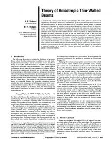
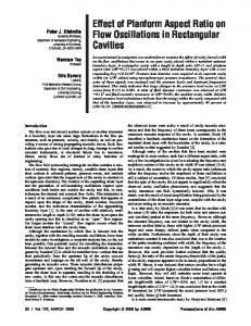
A rotational inverted pendulum system as described in 关12兴 is considered in this section. Figure 1 shows the physical model of the plant. The pendulum is composed of mass m 1 and inertia J 1 . l 1 is the distance to the center of gravity of the link from its pivot, g is the acceleration due to gravity, and C 1 is the frictional constant between the pendulum and the rotating base. The coordinate ␪ 0 represents the rotational angle of the base on the horizontal axis to a fixed point 共usually defined as the starting point兲 and ␪ 1 is the rotational angle of the pendulum to the vertical axis. ␪ 1 ⫽0 refers to the unstable equilibrium point. The dynamic equations of the system are represented by

再

␪¨ 0 ⫽⫺a p ␪˙ 0 ⫹K p u C1 m gl K ˙␪ 1 ⫹ 1 1 sin ␪ 1 ⫹ 1 ¨␪ 0 . ␪¨ 1 ⫽⫺ J1 J1 J1

K 1 ⬍0,

if ⫺ ␲ /2⬍ ␪ 1 ⬍ ␲ /2

K 1 ⬎0,

otherwise.

The applied armature voltage u is the only control input of the system. As addressed in 关12兴, the inverted pendulum system includes several control problems: swing-up, balancing, and both swing-up and balancing. In this paper, we will develop only a sliding mode controller for balancing control of the pendulum. The swing-up algorithm will be directly taken from 关12兴. First, we will try to stabilize the system such that the pendulum is in the unstable vertical position ␪ 1 ⫽0 and allow the base to be at an arbitrary fixed position. Then the design method will be generalized to drive both the pendulum and the rotating base to the equilibrium point ␪ 0 ⫽ ␪ 1 ⫽0 and maintain it there. 3.1 Control of the Inverted Pendulum. Notice, first, that in the system 共26兲 rewritten in the form 4 Õ Vol. 122, MARCH 2000

再

␪¨ 0 ⫽⫺a p ␪˙ 0 ⫹K p u ␪¨ 1 ⫽⫺

C1 m gl K K ˙␪ ⫹ 1 1 sin ␪ 1 ⫺ 1 a p ␪˙ 0 ⫹ 1 K p u, J1 1 J1 J1 J1 (27)

the control u is multiplied by constant coefficients. Since B(x) in this case is a constant matrix, a linear transformation is needed to reduce the system into a regular form. Let y⫽ ␪ 0 ⫺

J1 ␪ . K1 1

(28)

Differentiating Eq. 共28兲, one obtains y˙ ⫽ ␪˙ 0 ⫺

J1 ˙␪ K1 1

(29)

y¨ ⫽ ␪¨ 0 ⫺

J1 ¨␪ . K1 1

(30)

and

(26)

The upper equation is a simplified model of the permanent magnet DC motor used to drive the rotating base with constants a p and K p . The bottom part of system 共26兲 is the dynamics of the pendulum. K 1 is a proportionality constant. The sign of K 1 depends on the position of the pendulum, whether it is inverted or noninverted.

再

Fig. 1 The rotational inverted pendulum system

再

The motion equations are in the regular form C1 m gl ˙␪ 1 ⫺ 1 1 sin ␪ 1 K1 K1 a pK 1 m 1 gl 1 K 1K p C1 ␪¨ 1 ⫽⫺ ˙y ⫺ ⫹a p ␪˙ 1 ⫹ sin ␪ 1 ⫹ u. J1 J1 J1 J1 (31) y¨ ⫽

冉

冊

Let us first consider the lower subsystem of the regular form 共31兲 and try to stablize the system with respect to ␪ 1 ⫽0. For the discontinuous control u⫽⫺M sign共 s 兲 with s⫽ ␪˙ 1 ⫹c ␪ 1 ; c⬎0, both ␪˙ 1 →0 and ␪ 1 →0 as t→⬁ if sliding mode is enforced in the plane s⫽0. But, the zero dynamics of the pendulum 共from the upper equation of 共31兲兲 are given by y¨ ⫽0, hence y→⬁ as t→⬁, and the system is unstable. The conventional design approach 共case 1 in Sec. 2.3兲, therefore, does not work for the pendulum system if the control should stabilize the inverted pendulum in unstable vertical position with an arbitrary fixed position of the rotating base. Now, we try to design a sliding mode controller for the pendulum system based on the proposed design procedure of case 2, Sec. 2.3. Consider the upper equation of system 共31兲. According to Eq. 共19兲, the sliding manifold should be selected as Transactions of the ASME

m gl C1 ˙␪ ⫺ 1 1 sin ␪ 1 ⫽⫺c 1 y⫺c 2 y˙ , K1 1 K1

(32)

then the upper subsystem is stable,

s˙ ⫽cos ␪ 1 ␪¨ 1 ⫹ ␺ 1 共 x, ␪ 1 , ␪˙ 1 兲 ⫽

y¨ ⫽⫺c 1 y⫺c 2 y˙ , for positive parameters c 1 and c 2 . Both y→0 and y˙ →0 as t →⬁, however, as follows from the left-hand side of Eq. 共32兲, the zero dynamics of the reduced order system

␪˙ 1 ⫽

m 1 gl 1 sin ␪ 1 ; C1

m 1 gl 1 ⬎0 C1

C1 x⫽y˙ ⫺ ␪ K1 1

(33)

such that the right-hand side of the upper block in the motion equations would not depend on the time derivative of the state variable of the bottom block. Since x˙ ⫽y¨ ⫺(C 1 /K 1 ) ␪ 1 , substituting y¨ from system 共31兲, yields

冦

m 1 gl 1 sin ␪ 1 K1

␪¨ 1 ⫽⫺ ⫹

冉

冊

C1 a pK 1 a pC 1 x⫺ ␪ 1⫺ ⫹a p ␪˙ 1 J1 J1 J1

where ␺ 1 and ␺ ⬘1 are functions of the system states. Notice, that the function cos ␪1 is positive and parameter K 1 is negative for the pendulum angle ⫺ ␲ /2⬍ ␪ 1 ⬍ ␲ /2. The condition for existence of the sliding mode, s˙ s⬍0, is satisfied if

(34)

u 0⭓

(35)

3.2 Control of Both the Base Angle and Inverted Pendulum. We have just shown that the system can be stabilized with respect to ␪ 1 ⫽0 and ␪˙ 0 ⫽0 by introducing a new variable of x. Design of the control system for stabilizing both the pendulum and the rotating base at the equilibrium point ( ␪ 0 , ␪ 1 )⫽(0,0) is performed as follows. Step 1: The first equation of 共34兲 and Eq. 共33兲 constitute a system similar to Eq. 共24兲 in the design method of case 4

再

(36)

The derivative of s 1 does not depend on the control u

(40)

C1 ␪ . K1 1

(41)

再

x˙ ⫽⫺a 1 ␭ 1 共 x⫹y 兲 y˙ ⫽x⫹a 2 ␭ 1 h 共 ␪ 1 兲共 x⫹y 兲

(42)

where constants a 1 and a 2 for the inverted pendulum angle ⫺ ␲ /2⬍ ␪ 1 ⬍ ␲ /2 are positive defined as a 1 ⫽⫺

m 1 gl 1 ⬎0, K1

a 2 ⫽⫺

C1 ⬎0; K1

K 1 ⬍0,

(43)

and function h is a function of the pendulum angle ␪ 1 , h共 ␪1兲⫽

␪1 . sin ␪ 1

Stability of the system 共42兲 is analyzed using the Lyapunov function candidate

m 1 gl 1 sin ␪ 1 , K1

V⫽ 21 共 x⫹y 兲 2 ⫹ 21 x 2

but, it turns out to be a stable linear system of the first order s˙ 1 ⫽⫺ ␣ s 1

with V⫽0 at the origin (x,y)⫽(0,0). Taking the time derivative of the function and applying the system equations 共42兲, one obtains

if

␣ ⬎0.

(37)

Step 3: The condition 共37兲 is satisfied if sliding mode is enforced in the surface s⫽s˙ 1 ⫹ ␣ s 1 ⫽cos ␪ 1 ␪˙ 1 ⫺ ␣ 1

y˙ ⫽x⫹

with constant ␭ 1 , then the system is equivalent to

s 1 ⫽sin ␪ 1 ⫹ ␣ 1 x⫽0.

m 1 gl 1 sin ␪ 1 ⫽⫺ ␣ s 1 ; K1

m 1 gl 1 sin ␪ 1 K1

sin ␪ 1 ⫽⫺␭ 1 共 x⫹y 兲 ,

m 1 gl 1 a 1 ⫽⫺ K1

where a 1 ⬎0, since K 1 ⬍0 for ⫺ ␲ /2⬍ ␪ 1 ⬍ ␲ /2. It is a linear system and x→0 as t→⬁ for positive parameter ␣ 1 . In addition, since x decays exponentially, we can conclude from Eqs. 共29兲, 共33兲, and 共35兲 that functions ␪ 1 , y˙ , ␪˙ 1 , and ␪˙ 0 all exponentially decay as well. As a result, the desired system dynamics with ( ␪˙ 0 , ␪ 1 )→(0,0) as t→⬁ is obtained and the rotating base remains at a fixed position ( ␪ 0 ⫽const). Step 2: The condition 共35兲 holds if the function

cos ␪ 1 ␪˙ 1 ⫺ ␣ 1

x˙ ⫽⫺

The state component ␪ 1 in the system 共40兲 is handled as control. If the last term of the upper equation satisfies

holds, then the reduced order system becomes

s˙ 1 ⫽cos ␪ 1 ␪˙ 1 ⫺ ␣ 1

⫺J 1 兩 ␺ ⬘兩 . K 1 K p cos ␪ 1 1 ,max

Once the state trajectories of sliding mode are confined to the switching manifold s⫽0 after a finite time interval, s 1 →0 and x→0 as t→⬁. The desired dynamics behavior, ␪ 0 →const and ␪ 1 →0 as t→⬁, is guaranteed.

Now, it is obvious that the right-hand side of the upper equation in system 共34兲 does not depend on ␪˙ 1 . Following the approach of case 3, if the condition sin ␪ 1 ⫽⫺ ␣ 1 x

(39)

where

m 1 gl 1 K 1K p sin ␪ 1 ⫹ u. J1 J1

x˙ ⫽⫺a 1 ␣ 1 x;

K 1K p cos ␪ 1 u⫹ ␺ 1⬘ 共 x, ␪ 1 , ␪˙ 1 兲 J1

u⫽u 0 sign共 s 兲

are unstable. The case 2 in Sec. 2.3 is not applicable either. Try now to combine the ideas of cases 3 and 4 from Sec. 2.3. Step 1: Following the approach of case 4, we introduce a new variable

x˙ ⫽⫺

Since only the derivative of ␪˙ 1 depends on the control force u, one can obtain

m 1 gl 1 sin ␪ 1 ⫹ ␣ s 1 ⫽0. K1

V˙ ⫽ 共 x⫹y 兲共 x˙ ⫹y˙ 兲 ⫹xx˙ ⫽⫺ 关 a 1 ⫺a 2 h 共 ␪ 1 兲兴 ␭ 1 共 x⫹y 兲 2 ⫹x 共 x⫹y 兲 ⫺a 1 ␭ 1 x 共 x⫹y 兲 . (44) Thus, V˙ (t) is negative semi-definite

(38)


V˙ ⫽⫺ 关 a 1 ⫺a 2 h 共 ␪ 1 兲兴 ␭ 1 共 x⫹y 兲 2 ⭐0 MARCH 2000, Vol. 122 Õ 5

if ␭ 1⫽

1 ⬎0 a1

and the coefficient a 1 ⫺a 2 h 共 ␪ 1 兲 ⬎0.

(45)

The function h( ␪ 1 ) satisfies the inequalites 1⭐h 共 ␪ 1 兲 ⬍ ␲ /2

(46)

for pendulum angle ⫺ ␲ /2⬍ ␪ 1 ⬍ ␲ /2. Combining the inequalities 共45兲 and 共46兲 and substituting a 1 and a 2 from Eq. 共43兲, one obtains that the sufficient condition for the pendulum system to be stable is m 1 gl 1 ⬎ ␲ /2. C1

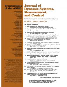
Fig. 2 Hardware setup configuration of the pendulum system

From a practical point of view, since the inverted pendulum is designed to rotate freely around its pivot 共no actuators are attached to the inverted pendulum兲, the frictional constant, C 1 , in general, is much less than the torque (m 1 gl 1 ) of the pendulum itself. Therefore, the condition 共45兲 holds for the pendulum system. Moreover, when V˙ ⫽0 or x⫹y⫽0, it follows from 共42兲 that x is a constant value, but y→⬁ as t→⬁ if this constant value is different from zero. Therefore, the system 共42兲 can maintain the V˙ ⫽0 condition only at the equilibrium point (x,y)⫽(0,0). It is shown that the equilibrium point is asymptotically stable in the large with x→0 and y→0 as t→⬁. Consequently, the control objective ( ␪ 0 , ␪ 1 )→(0,0) as t→⬁ is obtained from Eqs. 共28兲 and 共41兲. Step 2: Following the same procedure as described in the previous case, Eq. 共41兲 holds if the function

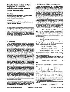
关6兴, special emphasis will be put on robustness by investigating the ability of the nonlinear controllers for significant plant parameter variations. The experimental setup used in this paper was developed, and it is currently available for both undergraduate and graduate control system laboratories at The Ohio State University. Figure 2 describes the complete hardware setup configuration of the inverted pendulum system. The real-time control system mainly consists of three parts: the controller, interface circuits, and the pendulum system. The controller is implemented as a C⫹⫹ program running on a 486 PC. Two optical encoders are used to measure the angular position of both the pendulum and the base. The sensor outputs are passed through a signal conditioning circuit before being acquired by the Lab Tender data acquisition board installed in the PC. A servo-amplifier is used to control the DC motor which applies a variable torque to the rotating base; this amplifier accepts control inputs from the DAS20’s D/A converter in the range of ⫾5 V. All parameters of the inverted pendulum system are listed in Table 1, and they are determined experimentally by identification techniques 共see 关12兴, for more details兲. The inverted pendulum system allows the user to change the system parameters, or add disturbances, by attaching containers of various size and contents to the end of the pendulum. A container of metal bolts and water will later be added to the pendulum in the set of experiments. The mass of the container and its contents significantly changes the system parameters, while the motion of the water within the container acts as a distributed disturbance to the system. Figure 3 shows the simulation results for stabilizing both the pendulum and the rotating base using the linear quadratic regulator 共LQR兲 technique: u⫽0.7␪ 0 ⫹1.0␪˙ 0 ⫹10.8␪ 1 ⫹0.7␪˙ 1 . The pendulum is first swung up with the swing-up algorithm, and then the LQR begins to take over the control when the rotational angle of the pendulum within the range of 兩 ␪ 1 兩 ⭐0.3 rad. The experimental results for nominal conditions by using the LQR has been provided both in 关12兴 and 关13兴. It has been observed that due to the unmodeled dynamics of the system 共e.g., sensor noise, sampling time, uncertainties, nonlinearities, etc.兲, the control input and some of the states do not ideally decay to zero.

s 1 ⫽sin ␪ 1 ⫹␭ 1 共 x⫹y 兲 ⫽0.

(47)

The function s 1 satisfies the linear first order differential equation s˙ 1 ⫽⫺␭s 1 ,

␭⬎0,

if cos ␪ 1 ␪˙ 1 ⫹␭ 1 共 x˙ ⫹y˙ 兲 ⫽⫺␭s 1 ,

(48)

since s˙ 1 ⫽cos ␪1␪˙ 1⫹␭1(x˙⫹y˙). Step 3: In order to satisfy Eq. 共48兲, sliding mode should be enforced in the switching manifold s⫽s˙ 1 ⫹␭s 1 ⫽cos ␪ 1 ␪˙ 1 ⫹␭ 1 共 x˙ ⫹y˙ 兲 ⫹␭s 1 ⫽0.

(49)

The time derivative of the function s is of the form s˙ ⫽cos ␪ 1 ␪¨ 1 ⫹ ␺ 2 共 x,y, ␪ 1 , ␪˙ 1 兲 ⫽

K 1K p cos ␪ 1 u⫹ ␺ ⬘2 共 x,y, ␪ 1 , ␪˙ 1 兲 J1

where ␺ 2 and ␺ ⬘2 are functions of the system states. The function cos ␪1 is positive and parameter K 1 is negative for the pendulum angle ⫺ ␲ /2⬍ ␪ 1 ⬍ ␲ /2. The condition for existence of the sliding mode 共the functions s and s˙ should have opposite signs兲 is satisfied if u⫽u 0 sign共 s 兲 ;

u 0⭓

⫺J 1 兩 ␺ ⬘兩 . K 1 K p cos ␪ 1 2 ,max

(50)

After sliding mode occurs on the surface s⫽0, s 1 →0 and (x,y) →(0,0) as t→⬁. Finally, the desired dynamics behavior, ( ␪ 0 , ␪ 1 )→(0,0) as t→⬁, is obtained.

4

Simulation and Experimental Results

Both simulation and experimental results for stabilizing the rotational inverted pendulum system will be presented in this section. Since simulation results of the sliding mode control for pendulum systems have been presented in the previous publication 6 Õ Vol. 122, MARCH 2000

Table 1 Parameters of the rotational inverted pendulum system Parameters/values

Parameters/values

l 1 ⫽0.113 m g⫽9.8066 m/s2 a p ⫽33.04

m 1 ⫽8.6184⫻10⫺2 kg J 1 ⫽1.301⫻10⫺3 N⫺m⫺s2 C 1 ⫽2.979⫻10⫺3 共N⫺m⫺s兲/rad ⫺1.9⫻10⫺3 , if ⫺ ␲ /2⬍ ␪ 1 ⬍ ␲ /2 K1⫽ 1.9⫻10⫺3 , otherwise

K p ⫽74.89

再

Transactions of the ASME

Fig. 3 Simulation results by LQR

Fig. 4 Simulation results by SMC for case 1: stabilizing the pendulum

Further, we will focus on the performance of the inverted pendulum system using our previously developed sliding mode controllers. Two case studies of the control objectives: case 1, stabilizing the pendulum at ␪ 1 ⫽0 with ␪˙ 0 ⫽0, and case 2, stabilizing both the pendulum and the rotating base with respect to the equilibrium point ␪ 0 ⫽ ␪ 1 ⫽0, will be presented.

and it is fixed for other experimental results in the later figures. The control law utilizing a continuous approximation by a sinusoidal function is designed as

4.1 Case 1: Stabilizing the Pendulum. The simulation results using the control law developed in Sec. 3.1 are shown in Fig. 4. The required information for calculating the control input are Eqs. 共29兲, 共33兲, 共36兲, 共38兲, and 共39兲. As can be seen, the pendulum angle is driven to zero, and the rotating base at the same time remains at a fixed position 共its angular velocity equals to zero兲 with the selected input gains ␣ 1 ⫽0.08, ␣ ⫽100, and u 0 ⫽3. The discontinuous controller was implemented for real-time control of the pendulum. We observed that due to the sampling issue of the discrete-time control system, in practice, the ideal sliding mode control cannot be implemented. Besides, as presented in many publications 关14–16兴, the chattering, which appears as a high-frequency oscillation at the vicinity of the desired manifold, may serve as a source to excite the unmodeled highfrequency dynamics of the system. In order to suppress the chattering problem, the saturating continuous approximation 关17,18兴 will be used in this paper to replace the ideal switching at the vicinity of the switching manifold. The problem of the tradeoff between accuracy and robustness are usually encountered after such substitution. Figures 5–7 are the experimental results of the SMC for stabilizing the pendulum with different loads attached at the end of the pendulum. Required system states ␪˙ 0 and ␪˙ 1 are obtained by taking the derivative of the rotational positions from the optical encoders. The sampling time for the control system is ⌬t⫽5 ms, Journal of Dynamic Systems, Measurement, and Control

u⫽

再

u 0 sin

冉冊

␲ s , 2␦

u 0 sign共 s 兲 ,

if 兩 s 兩 ⭐ ␦

(51)

otherwise.

where ␦ is the allowable maximum deviation of the continuous zone from the desired ideal sliding manifold s⫽0. It can be easily shown that the ideal discontinuous control is implemented when ␦ ⫽0. The larger the value of ␦, the less invariance of the system is anticipated; while, the less chattering in the system states is accomplished. The input gains of the SMC pendulum system are selected as: ␣ 1 ⫽0.08, ␣ ⫽400, and u 0 ⫽2.5. As can be seen in Fig. 5, for nominal plant the pendulum angle is stabilized close to zero. The control force input, as we expected, swings up the pendulum from the beginning, switches to the SMC at time around 1.5 s, and then stays in the ␦ zone 兩 u 兩 ⬍u 0 ⫽2.5 after 2 s. It should be noticed that since the control system with respect to the equilibrium point ( ␪˙ 0 , ␪ 1 )⫽(0,0) is marginally stable, the performance of the rotating base, because of the nonzero control input, presents slow drift 共␪ 0 is not constant兲. Similar results were obtained when the same controller 共51兲 is used to drive the pendulum with both the water 共Fig. 6兲 and the metal bolts 共Fig. 7兲. We observe that the controller can still manage the balance of the inverted pendulum quite well without saturation of the control input. The interesting differences are that small ripples are generated due to the distributed disturbance from the water in Fig. 6, average values of the control input in both cases gradually converge to zero when disturbances get settled at the final time 10 MARCH 2000, Vol. 122 Õ 7

Fig. 5 Experimental results by SMC: no weight „case 1…

Fig. 7 Experimental results by SMC: metal bolts „case 1…

s, and a smaller amplitude of the control input is observed at the steady-state when additional weight, the metal bolts, are added to the system as shown in Fig. 7.

Fig. 6 Experimental results by SMC: sloshing water „case 1…

8 Õ Vol. 122, MARCH 2000

4.2 Case 2: Stabilizing Both the Pendulum and the Base. The sliding mode control for stabilizing both the pendulum and the base will be designed following Eqs. 共28兲, 共29兲, 共33兲, 共47兲, 共49兲, and 共50兲. The simulation results by using the control law 共50兲 with the input gains of ␭ 1 ⫽0.08, ␭⫽800, and u 0 ⫽3 are shown in Fig. 8. Observe that the performance closely resembles that of the LQR in Fig. 3 in terms of the system states. The density of the discontinuous control input profile in some ranges is higher than that of the control input in Fig. 4. This is because additional control actions are applied for stabilizing the rotating base. Figure 9 shows the experimental results of the SMC for nominal pendulum using the modified controller 共51兲 with ␭ 1 ⫽0.08, ␭⫽800, and u 0 ⫽2.5. For a small value of ␦, we observe that the control input is still similar to the discontinuous function in Fig. 8, although its switching frequency is considerably reduced. As a result, the chattering exists in both of the state responses. The results for a larger value of ␦ are shown in Fig. 10. The control input is no longer saturated and it varies between the extreme values ⫾2.5. The most interesting experimental results are represented in Figs. 11 and 12. The controller is able to provide convergence under both the metal bolts and the sloshing water disturbances with the same gains in the control input. The system states are stabilized to the vicinity of the equilibrium point ( ␪ 0 , ␪ 1 ) ⫽(0,0). The low amplitude ripple similar to that in Fig. 6 under the effect of the sloshing water dynamics is still observed in Fig. 11, where the control input has an average value close to zero. We observe an underdamped system response in Fig. 12 for the pendulum with metal bolts. The control input oscillations are relaTransactions of the ASME

Fig. 8 Simulation results by SMC for case 2: stabilizing both the pendulum and the base

Fig. 10 Experimental results by SMC with larger ␦: no weight „case 2…

Fig. 9 Experimental results by SMC with small ␦: no weight „case 2…

Fig. 11 Experimental results by SMC: sloshing water „case 2…


MARCH 2000, Vol. 122 Õ 9

control approach which combines the regular form, block control principle, and sliding mode control techniques with the concept of zero dynamics, has been formulated for different configurations of the mechanical systems with either stable or unstable zero dynamics. Two case studies of the control objectives for stabilizing a rotational inverted pendulum system have been presented. It has been shown that the proposed design approach can be directly applied to mechanical systems governed by a set of second-order equations. Experimental results have demonstrated that the SMC approach has the advantages of invariance to both parameter variations and external disturbances.

Acknowledgments The authors would like to acknowledge The Control Systems Laboratory at The Ohio State University for experimental support of this research. They would also like to thank Professors K. Passino, V. Gazi, M. Moore, and Raul Ordonez for their assistance in hardware setup and helpful suggestions related to the research.

References

Fig. 12 Experimental results by SMC: metal bolts „case 2…

tively large at the beginning of the process compared with that of Fig. 7, but decrease to the same level after a couple of seconds when both the pendulum and the rotating base get settled.

5 Discussions We have just demonstrated the performance of the sliding mode control both in the simulation and experiment for the rotational inverted pendulum. We saw that the SMC using the proposed block control design principle is able to stabilize the nonlinear system at the equilibrium point from Section 4.2, and proves to be robust for unmodeled plant changes. Further investigations may be conducted to improve the discrepancy between the theoretical and experimental results. As mentioned in Section 4, nonlinearity was introduced to the system by the system states, ␪˙ 0 and ␪˙ 1 , which are both obtained by simply taking the derivative of the rotational positions from sensors. In addition, the approach, which has been applied to eliminate the chattering phenomenon caused by the nature of the discontinuous control input, is the saturating continuous approximation. Results from the experiment somewhat revealed the weakness of the continuous approach. The base angles for case 1 in Figs. 5–7 are unable to remain at a constant position with zero velocity, instead, move slowly to somewhat unbounded value. Also, the base angles in the case 2 oscillate within the ␦ zone of around 0.25 rad as seen in Figs. 10–12. One of the approaches, which has been proposed to suppress the chattering problem using the system knowledge with an asymptotic observer 关19兴, may be adopted to increase the accuracy of the control system states, while maintaining the robustness of the sliding mode control.

6

Conclusions

A generalized design procedure for the sliding mode control of nonlinear mechanical systems has been proposed. The proposed 10 Õ Vol. 122, MARCH 2000

关1兴 Luk’yanov, A. G., and Utkin, V. I., 1981, ‘‘Methods of Reducing Equations for Dynamic Systems to A Regular Form,’’ Autom. Remote Control 共Engl. Transl.兲, 42, pp. 413–420. 关2兴 Drakunov, S. V., Izosimov, D. B., Luk’yanov, A. G., Utkin, V. A., and Utkin, V. I., 1990, ‘‘The Block Control Principle I,’’ Autom. Remote Control 共Engl. Transl.兲, 51, pp. 601–608. 关3兴 Drakunov, S. V. Izosimov, D. B., Luk’yanov, A. G., Utkin, V. A., and Utkin, V. I., 1990, ‘‘The Block Control Principle II,’’ Autom. Remote Control 共Engl. Transl.兲, 51, pp. 737–746. 关4兴 Luk’yanov, A. G., 1993, ‘‘Optimal Nonlinear Block-Control Method,’’ Proc. of the 2nd European Control Conference, Groningen, pp. 1853–1855. 关5兴 Luk’yanov, A. G., and Dodds, S. J., 1996, ‘‘Sliding Mode Block Control of Uncertain Nonlinear Plants,’’ Proceedings of the 13th World Congress of the International Federation on Automatic Control (IFAC), San Francisco, CA, June 30–July 5. 关6兴 Utkin, V. I., Chang, H., Kolmanovsky, I., and Chen, D., 1998, ‘‘Sliding Mode Control Design based on Block Control Principle,’’ The Fourth International Conference on Motion and Vibration Control (MOVIC), Zurich, Switzerland, Aug. 25–28. 关7兴 Utkin, V. I., and Chen, D., 1998, ‘‘Sliding Mode Control of Pendulum Systems,’’ The Fourth International Conference on Motion and Vibration Control (MOVIC), Zurich, Switzerland, Aug. 25–28. 关8兴 Rashevskii, P. K., 1947, Geometrical Theory of Partial Differential Equations, Gostekhiiizdat, Moscow 共in Russian兲. 关9兴 Utkin, V. I., 1992, Sliding Modes in Control and Optimization, SpringerVerlag, Berlin. 关10兴 Utkin, V. I., 1977, ‘‘Variable Structure Systems with Sliding Modes,’’ IEEE Trans. Autom. Control, AC-22, pp. 212–222. 关11兴 Utkin, V. I., Drakunov, S. V., and Izosimov, D. B., 1984, ‘‘Hierarchical Principle of The Control System Decomposition Based on Motion Separation,’’ The 9th World IFAC Congress, Budapest, Hungary, July, 2–6. 关12兴 Widjaja, M., 1994, ‘‘Intelligent Control for Swing Up and Balancing of an Inverted Pendulum System,’’ Master’s thesis, The Ohio State University, Columbus, OH. 关13兴 Ordonez, R., Zumberge, J., Spooner, J. T., and Passino, K. M., 1997, ‘‘Adaptive Fuzzy Control: Experiments and Comparative Analyses,’’ IEEE Trans. Fuzzy Syst., 5, pp. 167–188. 关14兴 Utkin, V. I., 1978, Sliding Modes and Their Applications in Variable Structure Systems, Moscow, Mir. 关15兴 Kwatny, H. G., and Siu, T. L., 1987, ‘‘Chattering in Variable Structure Feedback Systems,’’ Proceedings of the 10th World Congress of the International Federation on Automatic Control (IFAC), Vol. 8, pp. 307–314. 关16兴 Bartolini, G., 1989, ‘‘Chattering Phenomena in Discontinuous Control Systems,’’ Int. J. Syst. Sci., 20, pp. 2471–2481. 关17兴 Slotine, J. J., and Sastry, S. S., 1983, ‘‘Tracking Control of Nonlinear Systems Using Sliding Surfaces, with Application to Robot Manipulators,’’ Int. J. Control, 38, pp. 465–492. 关18兴 Burton, J. A., and Zinober, A. S. I., 1986, ‘‘Continuous Approximation of Variable Structure Control,’’ Int. J. Syst. Sci., 17, pp. 875–885. 关19兴 Bondarev, S. A., Kostyleva, N. E., and Utkin, V. I., 1985, ‘‘Sliding Modes in Systems with Asymptotic State Observers,’’ Moscow, Translated from Automatika I Telemekhanika, pp. 5–11.


Christopher J. Damaren Associate Professor, Institute for Aerospace Studies, University of Toronto, 4925 Dufferin Street, Toronto, Ontario, M3H 5T6 Canada e-mail: [email protected]

1

Passivity and Noncollocation in the Control of Flexible Multibody Systems Collocation of actuation and sensing in flexible structures leads to the desirable inputoutput property of passivity which greatly simplifies the stabilization problem. However, many control problems of interest such as robotic manipulation are noncollocated in nature. This paper examines the possibility of combining collocated and noncollocated outputs so as to achieve passivity. An appropriate combination is shown to depend on the interplay between collocated and noncollocated mass properties. Tracking problems are also studied and a controller with adaptive feedforward elements is introduced. An experimental study using a simple flexible apparatus with one rigid degree of freedom and two vibration modes is used to validate the analysis. 关S0022-0434共00兲01701-9兴

Introduction

Many motion control problems are characterized by low mass structures which exhibit significant structural flexibility. There are often simultaneous requirements for control of rigid body motions coupled with active vibration suppression. Both problems are exacerbated by model uncertainty which necessitates the additional requirement of robustness. It has long been known that robust stabilization of both rigid and flexible structures can be readily achieved by collocating dual sets of 共rate兲 sensors and 共force兲 actuators. In this case, the inputoutput 共I/O兲 mapping is passive; in the linear time-invariant setting this manifests itself in the form of a positive real transfer function. Passivity and the positive real property were originally studied as characteristics of the driving point impedances of passive 共for example, RLC兲 circuits 关1兴. Stabilization of passive systems is readily achieved using strictly passive feedback as predicted by the passivity theorem 关2兴. This stability property is robust because the passivity of the I/O map is independent of the structural details, manner of spatial discretization, and number of modeled modes, but merely resides in the collocation assumption. One of the first to realize this was Gevarter 关3兴 who used simple proportional derivative 共PD兲 laws and eigenvalue perturbation arguments. Since then, many researchers have examined the collocated problem, but little research has investigated the exploitation of passivity for noncollocated inputs and outputs. Exceptions to this have typically focused on developing either static 关4兴 or dynamic 关5兴 output maps which yield a positive real system. In these cases, the required output transformation will be model dependent, but robustness can still be achieved by proper design of dynamic feedback compensation. The simplest compensator achieving stabilization for a passive plant is positive rate feedback, but this must be extended to proportional-integral 共PI or PD relative to position measurements兲 in the presence of rigid motions which lack stiffness. Benhabib et al. 关6兴 emphasized that compensation in the form of strictly positive real 共SPR兲 controllers could also furnish robust stability for passive systems and perhaps improve performance. Since then, many authors have established systematic procedures for SPR design 关7–10兴. Robotics problems, from the standpoint of joint-based control, furnish a class of systems exhibiting natural collocation and, although nonlinear, passivity has played an important role in the Contributed by the Dynamic Systems and Control Division for publication in the JOURNAL OF DYNAMIC SYSTEMS, MEASUREMENT, AND CONTROL. Manuscript received by the Dynamic Systems and Control Division September 22, 1999. Associate Technical Editor: N. Olgac.

development of controllers for setpoint regulation 关11兴 and both nonadaptive and adaptive tracking 关12兴. Space robotics has brought the problem of controlling flexible manipulators to the fore. In the archetypical form of the problem, one has a chain of flexible bodies with control inputs at the joints between bodies. However, the variables to be controlled are the position and orientation of the payload at the end of the manipulator. This represents a noncollocated problem requiring specialized approaches with serious limitations on achievable performance. It was in the study of that problem that the present author examined the ␮-output 关13兴. This is essentially a linear combination of collocated and noncollocated variables wherein ␮ ⫽0 yields the collocated case and ␮ ⫽1 gives the noncollocated one. The dependence of the passivity property on ␮ was studied in the asymptotic situation where the robot mass properties were negligible compared to those of the payload. Passivity was shown to be possible for ␮ ⬍1 and later work 关14兴 showed that this bound prevails for planar two- or three-link flexible manipulators with large payloads and/or large stators present at the end of each link. The present work serves to generalize the above by considering a finite noncollocated to collocated 共generalized兲 mass ratio. This incorporates other important mass effects such as the lumped rotor inertias associated with highly geared actuators. A critical value, ␮ 쐓 , is determined for which simple stabilization using the passivity theorem becomes possible for ␮ ⬍ ␮ 쐓 . In the case of multiple inputs and outputs, the analysis suggests the inclusion of a multiplier which defines the required spatial structure of the feedback controller. These enhancements greatly extend the applicability of the original ‘‘large payload’’ theory. For simplicity, linearized dynamics are introduced in Sec. 2 which affords access to modal analysis and the frequency domain. Passivity is studied in Sec. 3 as a function of ␮ and the interplay between collocated and noncollocated mass distributions. In addition, a controller containing feedforward elements is presented in Sec. 4 which provides adaptive tracking for prescribed trajectories of a certain output. Experimental results from an apparatus with a single rigid rotational degree of freedom and two dominant vibration modes will be used in Sec. 5 to validate the analysis.

2

Motion Equations and Input-Output Model

The motions of a flexible structure are assumed to be governed by the standard second-order motion equation Mq¨⫹Kq⫽Bf

(1)

where M, K, and B are the mass, stiffness, and input matrices, respectively. The N generalized coordinates q and these matrices are assumed be partitioned as


MARCH 2000, Vol. 122 Õ 11

M⫽

冋

Mrr

Mre

T Mre

Mee

册

,

K⫽

冋

O O

O Kee

册

,

B⫽

冋册

1 , O

q⫽

冋册

t

qr qe

(2)

Kee⫽KTee⬎O.

Hence, we identify qr with with M⫽M ⬎O and the N r rigid degrees of freedom, all of which are assumed to be actuated by N r generalized forces f. Rigid, as used here, denotes motions which are kinematically possible without storing any strain energy. The form of the input matrix B is consistent with the use of constrained 共also called appendage兲 modes or more general constrained shape functions for the N e elastic coordinates qe . That is, the elastic motions are kinematically subject to boundary conditions which are consistent with qr (t)⬅0. They correspond to motions which store strain energy in the system. The above description is sufficiently general to describe the linearized dynamics of an arbitrary elastic multibody system with complete actuation of the independent rigid degrees of freedom. The output of interest is assumed to be of the form ␳nc(t) ⫽ 关 Cr Ce 兴 q(t) where it is assumed that Cr is square and invertible. In the case of a flexible manipulator, ␳nc would be the generalized tip position 共relative to the linearization configuration兲 and Cr and Ce can be identified with the rigid and elastic Jacobian matrices. The subscript ‘‘nc’’ indicates ‘‘noncollocated’’ since, in general, the output of interest depends on qe and hence is not collocated with the control inputs f 共or u兲. Although there may be other configuration variables that are not collocated, the term noncollocated will be reserved for this special output. A more general output known as the ␮-rate can be identified: T

y共 t 兲 ⫽ ␳˙ ␮ ,Cr q˙r ⫹ ␮ Ce q˙e

(3)

where ␮ ⫽1 captures the true 共noncollocated兲 rates, ␳˙ nc , and ␮ ⫽0 constitutes an output ␳˙ co,Cr q˙r which is the natural dual of u(t),Cr⫺T f(t), an input more useful for our purposes. It is ˙ (q,q˙)⫽uT ␳˙ co⫽fT q˙r where H(q,q˙) straightforward to show that H is the Hamiltonian corresponding to Eq. 共1兲. Hence, f/q˙r and u/ ␳˙ co form collocated I/O pairs. For control purposes, it is assumed that ␳nc and ␳co 共via qr 兲 can be measured so that ␳␮ ⫽ ␮ ␳nc⫹(1 ⫺ ␮ ) ␳co can be formed. The eigenproblem corresponding to Eq. 共1兲 can be written as ⫺ ␻ ␣2 Mq␣ ⫹Kq␣ ⫽0,

␣ ⫽1,2,3,...

(4)

where ␻ ␣ are the unconstrained vibration frequencies and the q␣ ⫽col兵 qr ␣ ,qe ␣ 其 provide the corresponding modes shapes. There are N r zero-frequency rigid modes collectively of the form Qr ⫽ 关 1 O兴 T . The modes enjoy standard orthonormality relations with respect to M and K. Expanding the solution of Eq. 共1兲 and the output in Eq. 共3兲 in terms of eigenvectors, q(t)⫽Qr ␩r (t) Ne ⫹ 兺 ␣ ⫽1 q␣ ␩ ␣ (t), it is relatively straightforward to obtain the modal equations ¨ r ⫽f共 t 兲 ⫽CrT u, Mrr␩

␩¨ ␣ ⫹ ␻ ␣2 ␩ ␣ ⫽ 共 Cr qr ␣ 兲 T u共 t 兲 ,

(5)

␣ ⫽1,...,N e ,

(6)

兰 0f uT u dt⬍⬁. The system is passive if ⑀ ⫽0. For linear timeinvariant systems, this is equivalent to positive realness of the corresponding transfer function G(s), i.e., G(s) is analytic and G(s)⫹GH (s)⭓O for s in the open right-half plane. The transfer matrix in Eq. 共9兲 represents a linear combination of the positive real functions s ⫺1 and s/(s 2 ⫹ ␻ ␣2 ). It is known 关1兴 that such a function is positive real if and only if the coefficients, in this case Cr Mrr⫺1 CrT and c␣ b␣T , are positive-semidefinite. Clearly the first of these is always so and the entire issue resides in identifying situations where b␣ c␣T ⭓O for all modes. It occurs here for collocated feedback, i.e., ␮ ⫽0 so that b␣ ⫽c␣ ⫽Cr qr ␣ . The next section serves to enlarge the range of ␮ leading to passivity which has the further advantage of introducing the noncollocated output into the feedback.

3

Perturbation Analysis, Multipliers, and Passivity

Let us explicitly indicate the portion of the mass distribution associated with the noncollocated motion, ␳nc : M⫽

兺共C q

␣ ⫽1

˙␣ r r ␣ ⫹ ␮ Ce qe ␣ 兲 ␩

.

Using Laplace transforms, the dynamics of the system can be captured by the input-output description: y共 s 兲 ⫽G共 s 兲 u共 s 兲 ,

(8)

The ␦ notation is used to indicate quantities that are small to first order; Mnc⬎O is O(1) and assumed to be the dominant contribution to the mass distribution. It is representative of a massive manipulated object such as a large payload at the end of a lightweight robotic manipulator. The eigenvectors q␣ are decomposed as q␣ ⫽q ¯ ␣ ⫹ ␦ q␣

s 1 C M⫺1 CT ⫹ c bT , s r rr r ␣ ⫽1 s 2 ⫹ ␻ ␣2 ␣ ␣

兺

c␣ ⫽Cr qr ␣ ⫹ ␮ Ce qe ␣ ,b␣ ⫽Cr qr ␣ .

(9) (10)

Recall that a general square system is strictly passive if t t 兰 0f yT u dt⭓ ⑀ 兰 0f uT u dt for some ⑀ ⬎0, ᭙t f ⭓0, and ᭙u such that 12 Õ Vol. 122, MARCH 2000

(12)

where ¯q␣ is O(1) and ␦ q␣ denotes the first order perturbation due to ␦ M which we seek to uncover. Both ¯q␣ and ␦ q␣ can be partitioned analogously to q␣ . The ensuing analysis is equivalent to taking ␦ M 共M less the Mnc contribution兲 to be O(1) and taking Mnc to be O( ␦ ⫺1 ). In this light, ¯q␣ corresponds to the modes of the system with ␳nc⫽0 since as ␦ →0, the infinite contribution of Mnc acts as a clamping boundary condition for ␳nc . The first row in eigenequation 共4兲 implies that Mrrqr ␣ ⫹Mreqe ␣ ⫽0 or, upon substitution of the relevant partitions in Eqs. 共11兲 and 共12兲, 共 CrT MncCr ⫹ ␦ Mrr兲共 ¯qr ␣ ⫹ ␦ qr ␣ 兲 ⫹ 共 CrT MncCe ⫹ ␦ Mre兲共 ¯qe ␣ ⫹ ␦ qe ␣ 兲

⫽0.

(13)

Expanding and collecting terms of like order gives to

O共 ␦ 兲 :

CrT Mnc共 Cr¯qr ␣ ⫹Ce¯qe ␣ 兲 ⫽0;

CrT Mnc共 Cr ␦ qr ␣ ⫹Ce ␦ qe ␣ 兲 ⫹ ␦ Mrr¯qr ␣ ⫹ ␦ Mre¯qe ␣ ⫽0.

These imply that to O共 1 兲 : O共 ␦ 兲 :

Cr¯qr ␣ ⫽⫺Ce¯qe ␣ ;

(14)

⫺T Ce ␦ qe ␣ ⫽⫺ 关 Cr ␦ qr ␣ ⫹M⫺1 qr ␣ ⫹ ␦ Mre¯qe ␣ 兲兴 . nc Cr 共 ␦ Mrr¯

(15)

Ne

G共 s 兲 ⫽

(11)

T⫽ 21 ␳˙ TncMnc␳˙ nc⫹ 21 q˙T ␦ Mq.

O共 1 兲 : (7)

CrT Mnc关 Cr Ce 兴 ⫹ ␦ M CTe

where it is understood that ␦ M can be partitioned analogously to M in Eq. 共2兲. In other words, it is assumed that the kinetic energy can be written as

Ne

˙ r⫹ y共 t 兲 ⫽Cr ␩

冋册

The first of these implies that the noncollocated output is ‘‘clamped’’ in each vibration mode to O(1) in keeping with the assumption that Mnc forms the dominant contribution to the mass distribution. This follows from the definition of ␳nc which implies that Cr¯qr ␣ ⫹Ce¯qe ␣ is the relevant modal amplitude. Using these expressions in Eq. 共10兲, we can write Transactions of the ASME

c␣ bT␣ ⫽

再

共 1⫺ ␮ 兲共 Cr¯qr ␣ 兲共 Cr¯qr ␣ 兲 T , O共 1 兲 ; 共 1⫺ ␮ 兲 Cr 共 ¯qr ␣ ⫹ ␦ qr ␣ 兲共 ¯qr ␣ ⫹ ␦ qr ␣ 兲 T CrT ⫺T ⫺ ␮ M⫺1 qr ␣ ⫹ ␦ Mre¯qe ␣ 兲共 ¯qr ␣ ⫹ ␦ qr ␣ 兲 T CrT , nc Cr 共 ␦ Mrr¯

where the second of these is correct to the indicated order. The O(1) result shows that G(s) in Eq. 共9兲 is passive for ␮ ⬍1, but clearly ignores the correction stemming from ␦ M. The inclusion of the ␦ M effects in Eq. 共16兲 can improve the estimate on the range of ␮ leading to passivity. However, the term containing ␦ Mre presents an obstacle to further analytical progress but can be neglected in some cases. Using Eq. 共14兲, the bracketed expression in Eq. 共16兲 containing ␦ Mre can be written as

␦ Mrr¯qr ␣ ⫹ ␦ Mre¯qe ␣ ⫽ 关 ␦ Mre⫺ ␦ Mrr Cr⫺1 Ce 兴¯qe ␣ The term containing ␦ Mre can be neglected if 储 ␦ MrrCr⫺1 Ce 储 Ⰷ 储 ␦ Mre储 . This will happen when lumped rigid components associated with qr alone dominate ␦ Mrr . For example, rigid rotor inertias amplified by the use of large gear ratios contribute to ␦ Mrr but not ␦ Mre . The ensuing expression in 共16兲 can be simplified by defining Mco,Cr⫺T ␦ MrrCr⫺1 ,

Mt ,Mnc⫹Mco ,

(17)

⌼␮ , 关共 1⫺ ␮ 兲 1⫺ ␮ M⫺1 nc Mco兴 ,

(18)

cr ␣ ,Cr 共 ¯qr ␣ ⫹ ␦ qr ␣ 兲 .

(19)

Notice that the collocated mass matrix Mco represents the part of the mass distribution, less the Mnc contribution, associated with ␳co , assuming rigid bodies. Hence c␣ b␣T ⫽⌼␮ cr ␣ crT␣ , Mrr ⫽CrT (Mnc⫹Mco)Cr , Cr Mrr⫺1 CrT ⫽Mt⫺1 , and using Eq. 共9兲 Ne

G共 s 兲 ⫽s ⫺1 Mt⫺1 ⫹⌼␮

兺c

␣ ⫽1

T r ␣ cr ␣ 2

s

s ⫹ ␻ ␣2

.

(20)

In general, G is not positive real but the first term is and ⌼␮ premultiplies a summation which also is. The Single-Input Single-Output „SISO… Case „NrÄ1…. this case note that ⌼ ␮ ⫽1⫺

␮ , ␮쐓

␮ 쐓,

M nc ⬍1. M nc⫹M co

In

(21)

Therefore G(s) is passive if and only if ␮ ⬍ ␮ 쐓 When ␮ ⫽ ␮ 쐓 , the summation over the vibration modes vanishes 共all vibration modes become unobservable兲 and the output ␳˙ ␮ 쐓 ⫽Cr ␩ ˙ r becomes proportional to the rigid body modal rate. It is instructive to consider a small negative rate feedback u(t)⫽⫺ ⑀ ␳˙ ␮ . Using a simple eigenvalue perturbation argument, it is readily shown that the closedloop eigenvalues of each vibration mode are given by ⫺ ⑀ ⌼ ␮ crT␣ cr ␣ ⫾ j ␻ ␣ . All modes are stabilized when ␮ ⬍ ␮ 쐓 (⌼ ␮ ⬎0) and all of them are destabilized when ␮ ⬎ ␮ 쐓 (⌼ ␮ ⬍0) assuming controllability and observability, i.e., cr ␣ ⫽0.

(16)

O共 ␦ 兲 ,

In Sec. 4, the tracking problem will be considered and one must decide which output is to be prescribed. On the basis of the above, ␳␮ 쐓 is selected given the simple rigid nature of the I/O map. For ␮ ⬍ ␮ 쐓 , the I/O map is passive, hence minimum phase and causal inversion is possible. For ␮ ⬎ ␮ 쐓 , one expects nonminimum phase behavior and causal inversion would be impossible. In a certain sense, ␳˙ ␮ 쐓 is the closest output to ␳˙ nc whose I/O map can be inverted in a causal fashion. This will be further elucidated in Sec. 4. The Multivariable Case „NrÌ1…. In the multivariable case, it is helpful to consider the 共generalized兲 eigenproblem associated with the mass matrices: ␭ ␣ 共 Mnc⫹Mco兲 e␣ ⫽Mnce␣ ,

␣ ⫽1,...,N r .

(22)

Defining ⌳␮ ,diag兵␭␣其 and E,row兵 e␣ 其 , then with suitable normalization, ET (Mnc⫹Mco)E⫽1 and ET MncE⫽⌳␮ . Clearly ␭ ␣ ⬎0 and the eigenmatrix E will also diagonalize Mco . Using these ⫺1 ⫺1 and from Eq. 共18兲 relations, M⫺1 nc Mco⫽E(⌳␮ ⫺1)E ⌼␮ ⫽E⌬␮ E⫺1 ,

再

⌬␮ ,1⫺ ␮ ⌳␮⫺1 ⫽diag 1⫺

冎

␮ . ␭␣

(23)

If ␮ is chosen to satisfy eT Mnce ⬍1 T e⫽0 e Mt e

␮ ⬍ ␮ 쐓 ,min ␭ ␣ ⫽ inf ␣

(24)

then ⌬␮ is positive-definite. This definition of ␮ 쐓 generalizes that in Eq. 共21兲. ˆ ⫽G⌼␮T and G ¯ ⫽⌼␮⫺1 G are Lemma 1. The transfer matrices G positive real if ␮ ⬍ ␮ 쐓 . ˆ and G ¯ are of the Proof. Given the expression in Eq. 共20兲 both G form A0 s ⫺1 ⫹⌺ ␣ A␣ s/(s 2 ⫹ ␻ ␣2 ). It remains to show that A0 and ˆ , A␣ the A␣ are positive-semidefinite in each case. For G ¯ , A␣ ⫽cr ␣ crT␣ ⭓O. Now, note that ⫽⌼␮ cr ␣ crT␣ ⌼␮T ⭓O and for G Cr Mrr⫺1CrT ⫽(Mnc⫹Mco) ⫺1 ⫽EET . Using this in conjunction with ¯ , A0 ˆ , and for G Eq. 共23兲, A0 ⫽Cr Mrr⫺1 CrT ⌼␮T ⫽E⌬␮ ET for G ⫽⌼␮⫺1 Cr Mrr⫺1 CrT ⫽E⌬␮⫺1 ET . Both versions of A0 are positivedefinite when ␮ ⬍ ␮ 쐓 on account of ⌬␮ ⬎O. 䊐 Application of the Passivity Theorem. Using the notion of multipliers 关2兴, the feedback systems shown in Fig. 1 are equivalent from the point of view of stability. The passivity theorem states that if G is passive and H is strictly passive then r 苸L2 ⇒y苸L2 . Using Lemma 1 and the passivity theorem, the ˆ ⫽⌼␮⫺T H or H ¯ ⫽H⌼␮ is strictly original system is stable if either H passive. A possible design strategy would select Hsp , a strictly

Fig. 1 Equivalent feedback loops


MARCH 2000, Vol. 122 Õ 13

passive feedback, and then one would use either H⫽⌼␮T Hsp or H⫽Hsp⌼␮⫺1 . Either approach requires accurate knowledge of Mnc and Mco in forming ⌼␮ . Alternatively, if H(s)⫽(K d ⫹K p /s)Mco or H(s)⫽(K d ⫹K p /s)Mnc where K p ⬎0, K d ⬎0, it is readily shown using the ¯ are strictly passive ˆ and H previous eigendecompositions that H since ⌼␮⫺T Mco and Mnc⌼␮ are positive-definite matrices. The first of these is robust if Mnc is poorly known and the second is robust if Mco is poorly known. Both statements presuppose that ␮ is selected small enough. Other possibilities for H exist if the eigenstructure of Mnc and Mco is assumed known. In summary, stabilization is possible using a PD law whose spatial structure mirrors that of Mnc or Mco . This controller will be robust if ␮ ⬍ ␮ 쐓 where ␮ 쐓 could be determined using an upper bound for Mco or a lower bound for Mnc , respectively. The stability result is robust against variations in the stiffness properties and their manner of description but requires that 储 ␦ MrrCr⫺1 Ce 储 Ⰷ 储 ␦ Mre储 .

4

Feedforward Design and Adaptive Tracking

The development of a tracking controller is most readily accomplished in the time domain. A realization of the transfer matrix in Eq. 共20兲 is given by

¯ Te ud . ␩¨ d ⫹⍀2e ␩d ⫽C

(28)

This allows us to define the desired version of the ␮-output, ¯ e ␩d . ␳␮ d , ␳d ⫹⌼␮ C

(29)

Setting ˜␰r ⫽ ␰r ⫺ ␳d , ␩ ˜ e ⫽ ␩e ⫺ ␩d , ˜u⫽u⫺ud , and ˜␳␮ , ␳␮ ⫺ ␳␮ d , it is clear that the dynamics relating ˜u to ˜␳˙ ␮ are identical in form to those given by Eqs. 共25兲–共27兲 which relate u to y. Thus, ˜␳˙ ␮ (s)⫽G(s)u ˜ and is governed by the passivity results of the previous section. Stabilization of the error dynamics is then possible by taking ˜u⫽⫺⌼␮T Hsp˜␳˙ ␮ so that u共 t 兲 ⫽Mt ␳¨ d ⫺⌼␮T Hsp˜␳˙ ␮ .

(30)

Note that Hsp can simply be a PI law and ␳␮ (t) can be formed from ␮ ␳˙ nc⫹(1⫺ ␮ ) ␳˙ co , thus avoiding measurements of ␩e . Adaptive Case. In the case where Mt as needed in Eq. 共30兲 is poorly known but we have a lower bound on ␮ 쐓 , an adaptive tracking strategy can be established. The key resides in the notions of virtual trajectory and filtered error as originally introduced in a robotics context 关12兴. The desired feedforward is factored as ud ⫽Mt ␳¨ d ⫽W( ␳¨ d )a where the unknown, but assumed constant, parameters in Mt are contained in the column a and W is called the regressor matrix. Next, the virtual trajectory is defined by vr ⫽ ␳˙ d ⫺⌳˜␳␮ ,

⌳⬎O

(31)

Mt ␰¨ r ⫽u共 t 兲 ,

(25)

¯ Te u, ␩¨ e ⫹⍀2e ␩e ⫽C

(26)

ud ⫽W共 v˙r 兲 a⫽Mt 共 ␳¨ d ⫺⌳˜␳˙ ␮ 兲 ,

¯ e␩ y共 t 兲 ⫽ ␳˙ ␮ ⫽ ␰˙ r ⫹⌼␮ C ˙e ,

(27)

while ␩d continues to be defined by Eq. 共28兲. Subtracting Eq. 共32兲 from Eq. 共25兲 and Eq. 共28兲 from Eq. 共26兲, the error dynamics can be written as

and the feedforward is modified to read

¯ e ⫽row兵 cr ␣ 其 . Ideally, where ␩e ⫽col兵 ␩ ␣ 其 , ⍀e ⫽diag兵⍀␣其, and C we would like to find a control input u so that ␳nc tracks a desired trajectory ␳d which is prescribed along with ␳˙ d and ␳¨ d . To understand the difficulties associated with assigning ␳d to the desired behavior of ␳nc , let us adopt a quasistatic approximation for the elastic coordinates in Eq. 共26兲, i.e., neglect ␩¨ e . Such an approximation was shown to be highly effective in approximating the flexible motions produced by a complex simulation of the Space Shuttle Remote Manipulator System 关13兴. On this basis, ⫺2 ¯ T ¯T ¨ ␩e ⫽⍀⫺2 e Ce u⫽⍀e Ce Mt ␰r

where Eq. 共25兲 has been used for u. Substituting this into the integral of Eq. 共27兲 gives ¯ e ⍀⫺2 ¯T ¨ ␳␮ ⫽ ␰r ⫹⌼␮ C e Ce Mt ␰r If ␳d is assigned to the desired value of ␳␮ 共␳nc when ␮ ⫽1兲, then the above ODE can be used to determine the desired trajectory for ␰r . Assuming that ␳d begins at t⫽0, a causal trajectory for ␰r 共i.e., one that also begins at t⫽0兲, depends on the stability of the ODE. To keep things simple, consider the SISO case and recall that ⌼ ␮ ⫽1⫺( ␮ / ␮ 쐓 ). Stability 共causality of the I/O map from ␳d to ␰r 兲 requires that the coefficient of ␰¨ r above be positive which implies that ␮ ⬍ ␮ 쐓 . In general, a causal solution will not exist if ␮ ⫽1⬎ ␮ 쐓 , i.e., ␳␮ ⫽ ␳ nc . However, for ␮ ⫽ ␮ 쐓 , ␳␮ ⫽ ␰r since ⌼ ␮ ⫽0, so that the ␳ d can be identified with the desired behavior of the rigid 共modal兲 coordinate ␰r (t). Note that as ␮ 쐓 →1, so that ␮ can be taken close to 1, ␳␮ (t)⬟ ␰r (t)⬟ ␳nc(t) and hence ␳d is close to being the prescribed trajectory for ␳nc . Nonadaptive Case. Since ␳d (t) is the desired trajectory for ␰r (t), the nominal feedforward is selected to be ud ⫽Mt ␳¨ d according to Eq. 共25兲. The desired behavior for the elastic coordinates, ␩d , is determined using Eq. 共26兲: 14 Õ Vol. 122, MARCH 2000

¯ e␩ ˜␳␮ ⫽˜␰r ⫹⌼␮ C ˜e ,

再

(32)

Mt 共 ˜␰¨ r ⫹⌳˜␳˙ ␮ 兲 ⫽u ˜, ¯ Te ˜u. ␩ ˜¨ e ⫹⍀2e ␩ ˜ e ⫽C

(33)

Consider the following Lyapunov-like function: V⫽ 12 共 ˜␰˙ r ⫹⌳˜␳␮ 兲 T ⌼␮⫺T Mt 共 ˜␰˙ r ⫹⌳˜␳␮ 兲 ⫹ 21 ␩ ˜˙ Te ␩ ˜˙ e ⫹ 21 ␩ ˜ Te ⍀2e ␩ ˜ e ⭓0 (34) where ⌼␮⫺T Mt ⬎O since Mt⫺1 ⌼␮T ⬎O from the proof of Lemma 1. Using the error dynamics, its time derivative is V˙ ⫽( ˜␳˙ ␮ ⫹⌳˜␳␮ ) T ⌼␮⫺T˜u. Integration of this relationship establishes passivity between ⌼␮⫺T˜u and s␮ , ˜␳˙ ␮ ⫹⌳˜␳␮ which is termed the filtered error. If ⌼␮⫺T˜u is a strictly passive function of ⫺s␮ then s␮ 苸L2 . Using a well-known result, so are ˜␳˙ ␮ and ˜␳␮ . Hence, ␳¨ d can be replaced with v˙r and ˜␳˙ ␮ with s␮ in Eq. 共30兲 in the known parameter case: u共 t 兲 ⫽Mt v˙r ⫺⌼␮T Hsps␮ . In the case where a is poorly known, an estimate aˆ(t) can be employed: u⫽W共 v˙r 兲 aˆ⫹u ¯

(35)

where ¯u is the feedback portion of u. Subtracting Eq. 共32兲 from Eq. 共35兲 and defining ã,a ˜ ⫺a gives ⌼␮⫺T˜u⫽⌼␮⫺T 关 W(v˙r )aˆ⫹u ¯兴, which we would like to be a strictly passive function of ⫺s␮ , i.e., ⫺

冕

tf

0

冕冕

s␮T ⌼␮⫺T˜u dt⫽⫺ ⭓⑀

tf

0

tf

0

ãWT 共 v˙r 兲 T ⌼␮⫺1 s␮ dt⫺

s␮T s␮ dt.

冕

tf

0

s␮T ⌼␮⫺T¯u dt (36)

To this end, select Transactions of the ASME

ˆ t 关 ␳¨ d ⫺⌳共 ␳˙ ␮ ⫺ ␳˙ d 兲兴 ⫺Kd s␮ , u共 t 兲 ⫽Cr⫺T f⫽M

(38)

ˆ WT 共 v˙r 兲 s␮ , ⌫ ˆ ⫽ 共 1⫺ ␮ 兲 ⌫, aˆ˙⫽⫺⌫

(39)

where s␮ ⫽ ˜␳˙ ␮ ⫹⌳˜␳␮ with ˜␳␮ ⫽ ␳␮ ⫺ ␳d .

5

Fig. 2 Adaptive controller

¯u⫽⫺⌼␮T Kd s␮

共 Kd ⬎O兲 ,

ã˙ ⫽aˆ˙⫽⫺⌫WT 共 v˙r 兲 ⌼␮⫺1 s␮

共 ⌫⬎O兲 .

(37)

The first of these is strictly passive and the second represents a passive map (⌫s ⫺1 ) from WT ⌼␮⫺1 s␮ to ã. The overall system is shown in Fig. 2 and represents the negative feedback interconnecˆ and tion of a passive system 共the feedback interconnection of G the bottom adaptive loop, both of which are passive兲 and a strictly passive system Kd . Hence, s␮ 苸L2 and therefore ˜␳␮ , ˜␳˙ ␮ 苸L2 so that ˜␳␮ (t)→0 as t→⬁. Further arguments can be used to show ˜ e vanish as t→⬁. that ˜␳˙ ␮ , ˜␰r , and ␩ Implementation Issues. In the adaptive case, Mnc is assumed unknown and therefore so is ⌼␮ ⫽1⫺ ␮ (1⫺M⫺1 nc Mco) which is required to form the feedback and adaptation laws in Eq. 共37兲. However, if ⌼␮T Kd ⫽KMco (K⬎0) which does not require Mnc then Kd is positive-definite. The problem with the adaptation law can only be circumvented in certain cases. In the SISO situation, WT ⫽W and ⌼ ␮⫺1 commute so that ⌼ ␮⫺1 can be absorbed into the positive gain ⌫. A similar possibility exists in the multiple input multiple output 共MIMO兲 case if Mnc and Mco are diagonal so that W and ⌼␮ can be taken to be diagonal. Otherwise, it is proposed to approximate ⌼␮ by (1⫺ ␮ )1 and absorb it into ⌫. Another drawback is the calculation of ␩d in Eq. 共28兲 which requires ud based on the true parameters. We propose to take ␳␮ d ⬟ ␳d , an approximation which improves as ␮ → ␮ 쐓 . The final form of the controller incorporating these modifications is

Experimental Results

The control strategy developed in the previous section was implemented on the Torsional Control System apparatus developed by Educational Control Products. It consists of three concentric disks which are separated by two thin steel wires of length 305 and 310 mm 共see Fig. 3兲. The wires are effectively modeled as massless lumped torsional stiffnesses k 1 and k 2 . Each of the three disks can be removed or augmented with brass masses of variable position which allows one to systematically vary the axial moment of inertia of each disk (J 1 ,J 2 ,J 3 ). The base disk is free to rotate and is driven by a brushless DC motor. Angular encoders 共4000⫻4 counts per revolution兲 are used to sense the rotational motion of each disk ( ␪ 1 , ␪ 2 , ␪ 3 ). Torque control of the motor is accomplished with a high gain PI current loop which has a bandwidth of 500 Hz. The apparatus is interfaced to a DSP which resides on the PC backplane and user written control algorithms can be developed on the PC and downloaded to the DSP. If q r ⫽ ␪ 1 , q e1 ⫽ ␪ 2 ⫺ ␪ 1 , and q e2 ⫽ ␪ 3 ⫺ ␪ 2 are selected as generalized coordinates and f (t) as the motor torque, the matrices defined in Eq. 共2兲 are given by M⫽

冋

册冋

J 1 ⫹J 2 ⫹J 3

J 2 ⫹J 3

J3

J 2 ⫹J 3

J 2 ⫹J 3

J3 ,

J3

J3

J3

冋册

册

0

0

0

K⫽ 0

k1

0 ,

0

0

k2

1 B⫽ 0 . 0

(40)

The noncollocated degree of freedom is taken to be ␳ nc⫽ ␪ 3 ⫽ ␪ 1 ⫹ 关 1 1 兴 qe so that Cr ⫽1, Ce ⫽ 关 1 1 兴 . The collocated degree of freedom is ␳ co⫽ ␪ 1 and ␳ ␮ ⫽ ␮␪ 3 ⫹(1⫺ ␮ ) ␪ 1 . Nominally, disks 1 and 2 were removed reducing J 1 and J 2 to their minimum values and the maximum number of masses 共4兲 were placed on disk 3 in their most outboard position. The corresponding parameter values are given in Table 1. The calculated

Fig. 3 Torsional control system apparatus „reprinted courtesy of Educational Control Products…


MARCH 2000, Vol. 122 Õ 15

Table 2 Measured values of ␮ cr at stability-boundary

Table 1 Torsional apparatus parameter values k 1 ⫽2.8 N•m/rad, k 2 ⫽2.7 N•m/rad J 1 ⫽0.508 g•m2, J 2 ⫽0.008 g•m2, J 3 ⫽18.725 g•m2

J 1 共g•m2兲

J 2 共g•m2兲

J 3 共g•m2兲

␮쐓

␮ cr

0.508 2.408 6.233 9.083 14.283 19.233 2.408 19.233 7.083 17.483

0.008 0.008 0.008 0.008 0.008 1.908 0.008 0.008 0.008 0.008

18.725 18.725 18.725 18.725 18.725 18.725 1.900 9.438 1.900 1.900

0.973 0.886 0.750 0.673 0.567 0.470 0.440 0.329 0.211 0.098

0.973 0.889 0.772 0.688 0.584 0.563 0.462 0.370 0.277 0.135

Fig. 4 Tracking errors „␮ 쐓 Ä0.973, ␮ Ä0.96…

Fig. 6 Tracking errors and parameter estimates „␮ 쐓 Ä0.567, ␮ Ä0.55…

Fig. 5 Parameter estimates „␮ 쐓 Ä0.973, ␮ Ä0.96…

natural frequencies for this configuration were ␻ 1 ⫽8.3 Hz and ␻ 2 ⫽113 Hz, both of which were validated experimentally to within 1%. For this structure M nc⫽J 3 and M co⫽J 1 ⫹J 2 so that ␮ 쐓 ⫽M nc /(M nc⫹M co)⫽0.973 for the parameter values in Table 1. All controllers were implemented with a sampling period of T s ⫽0.003536 s and the derivatives ␪˙ 1 and ␪˙ 3 required to form ␳˙ ␮ were obtained by simple differencing of the encoder measurements. Initially a PD law of the form f (t)⫽⫺K d s ␮ , s ␮ ⫽˜␳˙ ␮ ⫹⌳˜␳ ␮ , ˜␳ ␮ ⫽ ␳ ␮ ⫺ ␳ d was employed with K d ⫽0.605 N•m•s/rad/s, ⌳⫽11.3 s⫺1, and ␳ d ⫽0. This places the eigenvalues of the rigid mode at ⫺15.7⫾ j10.4 rad/s when ␮ ⫽ ␮ 쐓 . The stability boundary was found to occur experimentally at ␮ cr⫽0.973 which is identical to the calculated value of ␮ 쐓 . For analysis of the tracking problem, the desired trajectory ␳ d (t) was a quintic polynomial taking ␳ d from 0 to 180 deg in T⫽1 s with ␳˙ d (0)⫽ ␳˙ d (T)⫽ ␳¨ d (0)⫽ ␳¨ (T)⫽0. For 1 s⭐t⭐2 s, a similar maneuver takes ␳ d from 180 deg back to 0 and for t ⭓2 s, the entire maneuver repeats itself with a period of 2 s. The use of the simple PD law for tracking is shown in Fig. 4 ( ␮ ⫽0.96) and the tracking error is on the order of ⫾4 deg. If this is augmented with the feedforward given in Eq. 共30兲, i.e., f (t) ⫽M t ␳¨ d ⫺K d s ␮ , M t ⫽J 1 ⫹J 2 ⫹J 3 , the tracking performance is greatly improved as shown in Fig. 4. Setting W( ␳¨ d )⫽ ␳¨ d , a⫽M t , the adaptive form f 共 t 兲 ⫽W 共 v˙ r 兲 aˆ ⫺K d s ␮ , aˆ˙ ⫽⌫W 共 v˙ r 兲 s ␮ 16 Õ Vol. 122, MARCH 2000

(41)

Fig. 7 Experimental and theoretical stability regions

was implemented with ⌫⫽12.4 g•m2•s2, which yields an average time constant for the adaptation of 0.63 s. The tracking performance for aˆ (0)⫽0 is also given in Fig. 4 and is nearly as good as the fixed parameter case. This is excellent considering the speed of the maneuver and the flimsy nature of the structure separating the control input and the manipulated inertia. The behavior of the estimate aˆ (t) is shown in Fig. 5. Notice that it oscillates about the true value on account of unmodeled effects such as drive and support joint friction. If this is modeled in the regressor by taking ˆ t ,D ˆ t 其 where D ˆ t is interpreted as an effecW⫽ 关v˙ r v r 兴 , aˆ⫽col兵 M Transactions of the ASME

ˆ t improves to that tive viscous damping constant, the estimate M given in Fig. 5. The tracking error in Fig. 4 showed little change but further improvement is possible by attributing separate damping constants to ␪˙ 1 and ␪˙ 3 . Next, the controller in Eq. 共41兲 was implemented for various values of J 1 , J 2 , and J 3 which were achieved by varying the location of the masses on J 3 and/or J 1 . The critical value of ␮ 쐓 is tabulated in Table 2 along with the observed values of ␮, ␮ cr , which led to instability. In each case, stability was achieved for values of ␮ ⬍ ␮ cr . The agreement is quite good despite the fact that ␮ 쐓 was determined using first order perturbation theory which assumes that M ncⰇM co . The worst case occurs for ␮ 쐓 ⫽0.470 which corresponds to including disk 2. This is not surprising since ␦ Mre⫽ 关 J 2 0 兴 which was neglected in the analysis. The tracking and adaptation performance are shown in Fig. 6 for the case where ␮ 쐓 ⫽0.567 and a value of ␮ ⫽0.55 was used. Notice that ␪ 3 tracks ␳ d to within 12 deg in the steady state, but one must bear in mind that ␳ d is the prescribed behavior of ␳ ␮ 쐓 . The error ˜␳ ␮ is also shown in Fig. 6 and is considerably smaller. The information conveyed by Table 2 in conjunction with Eq. 共21兲 is summarized by the stability diagram in Fig. 7. Here, ‘‘stable’’ and ‘‘unstable’’ refer to the use of a strictly passive feedback and the values of ␮ cr refer more specifically to the adaptive PD law used here. The most important feature of the diagram aside from the closeness of ␮ cr and ␮ 쐓 is the conservative nature of the prediction from Eq. 共21兲, i.e., ␮ 쐓 ⭐ ␮ cr in all cases.

6

Concluding Remarks

A theory of control for flexible structures performing rigid body motions with noncollocated outputs and inputs has been presented. By judiciously combining collocated and noncollocated measurements, it has been shown that passivity can be achieved in the appropriate I/O map. Provided a lower bound on ␮ 쐓 is known, robust stabilization and tracking are possible using simple PD controllers. An adaptive form of the tracking controller performed excellently for an experimental system with one rigid degree of freedom and all theoretical predictions were validated. The multivariable form of the control laws was established here and suggests the use of a PD controller whose feedback gains mirror the spatial


structure of either the noncollocated or collocated mass matrix. Multibody problems with large rigid motions bring significant nonlinearities into play. Future work will address experimental implementation of the proposed controllers on flexible manipulators carrying large payloads.

Acknowledgment The author gratefully acknowledges financial support provided by the University of Canterbury in the form of Research Grant 2201999.

References 关1兴 Newcomb, R. W., 1966, Linear Multiport Synthesis, McGraw-Hill, New York. 关2兴 Desoer, C. A., and Vidyasagar, M., 1975, Feedback Systems: Input-Output Properties, Academic Press, New York. 关3兴 Gevarter, W. B., 1970, ‘‘Basic Relations for Control of Flexible Vehicles,’’ AIAA J., 8, pp. 666–672. 关4兴 Hughes, D., and Wen, J. T., 1996, ‘‘Passivity Motivated Controller Design for Flexible Structures,’’ AIAA J. Guid. Control Dynam., 19, pp. 726–729. 关5兴 Lee, F. C., Flashner, H., and Safonov, M. G., 1995, ‘‘Positivity-Based Control System Synthesis Using Alternating LMIs,’’ Proceedings of American Control Conference, Seattle, WA, American Automatic Control Council, Evanston, IL, pp. 1469–1473. 关6兴 Benhabib, R. J., Iwens, R. P., and Jackson, R. L., 1981, ‘‘Stability of Large Space Structure Control Systems Using Positivity Concepts,’’ AIAA J. Guid. Control, 4, pp. 487–494. 关7兴 McLaren, M. D., and Slater, G. L., 1987, ‘‘Robust Multivariable Control of Large Space Structures Using Positivity,’’ AIAA J. Guid. Control Dynam., 10, pp. 393–400. 关8兴 Lozano-Leal, R. and Joshi, S. M., 1988, ‘‘On the Design of Dissipative LQGType Controllers,’’ Proc. 27th IEEE Decision and Control Conference, Dec., 2, pp. 1645–1646. 关9兴 Haddad, W. M., Bernstein, D. S., and Wang, Y. W., 1994, ‘‘Dissipative H 2 /H ⬁ Controller Synthesis,’’ IEEE Trans. Autom. Control., 39, pp. 827– 831. 关10兴 Damaren, C. J., 1996, ‘‘Gain Scheduled SPR Controllers for Nonlinear Flexible Systems,’’ ASME J. Dyn. Syst., Meas., Control, 118, pp. 698–703. 关11兴 Takegaki, M. and Arimoto, S., 1981, ‘‘A New Feedback Method for Dynamic Control of Manipulators,’’ ASME J. Dyn. Syst., Meas., Control, 103, pp. 119– 125. 关12兴 Ortega, R. and Spong, M. W., 1989, ‘‘Adaptive Motion Control of Rigid Robots: A Tutorial,’’ Automatica, 25, pp. 877–888. 关13兴 Damaren, C. J., 1995, ‘‘Passivity Analysis for Flexible Multilink Space Manipulators,’’ AIAA J. Guid. Control Dynam., 18, pp. 272–279. 关14兴 Damaren, C. J., 1998, ‘‘Modal Properties and Control System Design for Two-Link Flexible Manipulators,’’ Int. J. Robot. Res., 17, pp. 667–678.

MARCH 2000, Vol. 122 Õ 17

P. Tomas Larsson A. Galip Ulsoy Department of Mechanical Engineering and Applied Mechanics, University of Michigan, Ann Arbor, MI 48109-2125

1

Fast Control of Linear Systems Subject to Input Constraints Efficient design of high performance automatic control systems is extremely important for high technology systems. To get the best hardware cost-to-performance ratio, it is desirable to design a controller that takes full advantage of actuator capabilities, but this can lead to nonlinear behavior due to actuator saturation. The saturation nonlinearities in the system may have severe effects on system performance due to, for example, integrator windup. In this paper, a new design method is presented based on Lyapunov stability theory. By incorporating the actuator constraints directly in the design method, better utilization of the available control effort can be ensured in achieving desired system behavior. 关S0022-0434共00兲01801-3兴

Introduction

Every physical control system has some kind of actuator limitation or nonlinearity 共e.g., a motor can only supply limited torque and limited power兲. The actuator limitation ultimately limits the achievable closed-loop performance. Often, actuator constraints impose more severe performance limitations than other sources such as modeling uncertainties 关1兴. The effects of amplitude saturation have been extensively studied for decades, but it is not the only type of actuator saturation. Recently, increasing work has been done on the control of systems where the output rate of change of the actuator is limited 共e.g., 关2–4兴.兲 Power saturation depends on the product of two states 共e.g., voltage and current兲. Other constraints are internal to the plant. A plant state variable could, for example, be limited for safety reasons. The design method presented in this paper deals with the design of linear systems with input amplitude saturation. However, it can be extended to handle other types of constraints. The traditional design approach for systems with amplitude saturation has two-steps: A linear controller is designed first, ignoring the effects of actuator saturation, and then an ad hoc antiwindup 共AW兲 scheme is designed to reduce the problems that arise due to saturation nonlinearities. Since the constraints are not considered in the linear design it may not take full advantage of the available actuator capacity. Since the most severe wind-up problems often come from integral control, that is where much attention has been focused. See, e.g., the research on proportionalintegral-derivative 共PID兲 controllers in 关5–9兴. Another approach is to use guaranteed domains of attraction 共GDA兲共invariant sets兲 to design a reference governor that restricts the reference signal to avoid saturation, see 关10兴. See also 关11兴, which uses GDA:s to avoid saturation by switching between increasingly ‘‘faster’’ controllers as the states approaches the set point. The design procedure presented in this paper can be applied to both full-state feedback and full-state feedback plus integral control for single-input single-output 共SISO兲 systems. When integral control is used, a simple AW scheme is added to improve system performance. First, the general design concept will be described. Second, several design examples are presented. They include simulation and experimental results that support the design approach. Additional examples that support the feasibility of the design method can be found in 关12兴. The ideas presented in this paper are closely related to work presented in 关13兴 and 关14兴, where the goal is to design a saturating controller that fully utilizes available control effort while optimizContributed by the Dynamic Systems and Control Division for publication in the JOURNAL OF DYNAMIC SYSTEMS, MEASUREMENT, AND CONTROL. Manuscript received by the Dynamic Systems and Control Division July 14, 1998. Associate Technical Editor: T. R. Kurfess.

18 Õ Vol. 122, MARCH 2000

ing performance. See 关15兴 for a method that results in a guaranteed cost in the presence of saturation. The design method presented in this paper differs in that the emphasis is on achieving a desired linear behavior, instead of robustness to saturation.

2

Assumptions The plant is given by the discrete-time system x共 t⫹1 兲 ⫽Ax共 t 兲 ⫹Bsat共 u 共 t 兲兲 ,

(1)

y共 t 兲 ⫽C1 x共 t 兲 ,

(2)

z 共 t 兲 ⫽C2 x共 t 兲 ,

(3)

n

with state x苸R , controlled output z苸R, output measurement y苸Rn , and actuator output u苸R. The saturation function is defined by sat共 u 兲 ⫽

再

u,

if abs共 u 兲 ⭐u max

sign共 u 兲 u max ,

if abs共 u 兲 ⬎u max

(4)

It is assumed that u max , is known. C1 is the identity matrix so that full state feedback, u⫽⫺Kx⫽⫺Ky

(5)

can be used. The reference input is assumed to be zero. If C1 ⫽I, the design method can still be used by designing a state observer. See 关16兴 for a discussion on the effect of the design of the observer on the proposed design method.

3

The Design Concept

In most research on saturating control it is assumed that a good linear design already exists, and the emphasis is on finding a method to minimize the effect of the saturation element on the system performance. The emphasis here is different, in that there is no a priori linear design. The goal of the design is to come up with a linear controller that with saturation minimizes the settling time of the system. A key idea is the scaling of the linear design by a parameter ␤⬎0 which is chosen so that the system performance improves as ␤ increases. It was shown in 关17兴 how such a dependency on ␤ can be achieved using linear quadratic regulator 共LQR兲 design. To make things specific, let the performance be measured by the settling time and choose the scaling parameter by pole placement. Specifically, suppose ␤ is determined by the following procedure: 1 Define vector of complex pole locations pb that results in a desirable system behavior. 2 Introduce a real scalar scaling parameter ␤ such that the final

Copyright © 2000 by ASME


Fig. 1 Scaling of poles

pole locations pc are defined by pc ⫽ ␤ pb 共see Fig. 1兲, or if discrete time control is used pc ⫽e ⫺ ␤ pb ⌬T , where ⌬T is the sampling time. This way of scaling maintains the damping of the poles, while changing the speed of the response. 3 Choose the feedback gains K( ␤ ), so that the closed loop poles are given by pc . This simple scaling idea is fine for many plants. Indeed, the performance cost 共settling time兲 will often be reduced as ␤ increases. In general, though, a more advanced form of scaling will be needed, such as the LQR based method in 关17兴. For example, if the plant transfer function has poorly placed zeros, the overshoot and hence the settling time might increase as ␤ is increased. The vector pb is assumed given and the nontrivial problem of how to choose it are not addressed here. The method of scaling is not critical to the design method as long as the performance cost is a monotone decreasing function of ␤. Clearly, if the control signal does not saturate, it is desirable to increase ␤. In the presence of saturation there will be a limit to the achievable performance, but that limit is generally not given by the onset of saturation. Figure 2 shows the 1 percent settling time, as a function of ␤, for the digital state feedback control of a double integrator plant: pb ⫽ 关 ⫺1,⫺1 兴共i.e., a critically damped design兲, for an initial position displacement of 1, and a sampling time of 0.01 s. From Fig. 2 it is clear that the performance can be improved by increasing ␤ outside the interval (0,␤ lin) where the control does

not saturate. However, as ␤ is increased beyond ␤ opt the behavior of the system starts to deteriorate due to saturation effects. Similar results can be obtained using other performance measures, such as the integral of the squared error. The extent to which the behavior can be improved relative to the nonsaturating case are highly dependent on the dynamics of the open loop plant. The success of a controller designed in this manner may vary. The 1 percent settling time for the time optimal bang-bang control for the above example is 1.8 s, and, as can be seen from Fig. 2, it is possible to get quite close to that time by just using a linear feedback and letting it saturate. Of course, the time-optimal control reaches the set-point in finite time, whereas the linear saturating controller asymptotically approach the set-point. Similar conclusions have been drawn in 关18兴 for the proportional-derivative 共PD兲 control of second order systems. They show it is possible to increase the closed-loop bandwidth and decrease the root mean square 共RMS兲 error by choosing PD feedback gains so that the controller saturates. Since the design has been parameterized by a single design parameter ␤ it is easy to do a search over ␤ to find the optimal value for a particular initial condition 共or step input size兲. In general, it is desirable to have a good response for a set of initial conditions, not just one particular initial condition. In this case, it is natural to minimize the worst case settling time, i.e.,

␤ opt⫽arg min共 max t s 兲 , ␤

(6)

x 0 傺IC

where IC is the specified set of initial conditions. While the optimal solution to Eq. 共6兲 may be achieved numerically for systems of very low order by repeated simulation, it is generally intractable. Another disadvantage of trying to solve Eq. 共6兲 is that nothing is known about the robustness of the design. Another approach, which circumvents Eq. 共6兲 is to construct a guaranteed domain of attraction, ⍀ s ( ␤ ). The ‘‘size’’ of ⍀ s ( ␤ ) generally becomes smaller as ␤ increases. The idea is to maximize ␤ under the constraint that IC傺⍀ s ( ␤ ). The resulting value of ␤ is

␤ sat⫽ max ␤ .

(7)

IC傺⍀ 共 ␤ 兲

While it is generally true that ␤ sat is less than ␤ opt , solving for ␤ sat is numerically feasible and it can produce efficient designs. Moreover, designs can also be made robust to disturbances and parameter uncertainties 共see 关16兴兲. A method for constructing ellipsoidal GDA’s is described in the following section. Notice that as long as a monotone dependence between a scalar design parameter and a performance cost can be identified any linear design technique 共state space or frequency domain兲 can be used to do the scaling. In this paper, pole placement is used to perform the scaling for the initial examples, and LQR design is used to do the scaling for the experimental setup.

4

A Guaranteed Domain of Attraction

First, we state a theorem that for fixed K determines an ellipsoidal domain of attraction for the saturated feedback system determined by Eqs. 共1兲–共5兲. The proof depends on a simple application of the discrete-time Lyapunov equation. The proof for the continuous-time case can be obtained by using the continuoustime Lyapunov equation instead of the discrete time Lyapunov equation. Given an m⫻m, positive definite symmetric matrix P, and a feedback gain K that stabilizes the system x(t⫹1)⫽(A ⫺BK)x(t), let 0⬍ ␣ min⬍1, be a number such that the matrix inequality 共 A⫺ ␣ BK兲 T P共 A⫺ ␣ BK兲 ⫺P⬍⫺ ⑀ I

Fig. 2 Scaling design for PD control of a double integrator plant


(8)

is satisfied for all ␣ 苸关 ␣ min,1兴 , for a fixed P, and for an arbitrarily small constant ⑀ ⬎0. Note that ␣ min will depend on K and P. A necessary condition for the existence of a matrix P that satisfies Eq. 共8兲 for all ␣ 苸关 ␣ min,1兴 is that all the eigenvalues of the matrix A⫺ ␣ BK are placed inside the unit disk for ␣ 苸关 ␣ min,1兴 . MARCH 2000, Vol. 122 Õ 19

Theorem 4.1. Define

␥ , 共 KP

⫺1

2 ⫺2 KT 兲 ⫺1 u max ␣ min

(9)

and ⍀ s 共 K,P兲 , 兵 x苸Rn 兩 xT Px⭐ ␥ 其

(10)

x共 t⫹1 兲 ⫽A⫺Bsat共 Kx共 t 兲兲

(11)

Then the system has an asymptotically stable equilibrium point at x⫽0 and ⍀ s is a guaranteed domain of attraction. Specifically, x(0)苸⍀ s implies x(t)苸⍀ s for all t⬎0 and x共 t 兲 →0 as t→⬁

(12)

Proof: First we show that x苸⍀ s implies sat(Kx)⫽ ␣ (x)Kx where ␣ min⭐␣(x)⭐1. It is clear that ␣共x兲⫽1 when 兩 Kx兩 ⭐u max and ␣共x兲 is minimum when 兩Kx兩, x苸⍀ s , is maximum. The condition ␣ min⭐␣(x) is achieved by choosing ␥ appropriately. The maxx苸⍀ s Kx exists since ⍀ s is compact. Moreover, a maximizing state x* must satisfy the multiplier rule for inequality constraints: ␭ⵜKx⫽ⵜ(xT Px⫺ ␥ ) at x⫽x*, ␭⭓0. Equivalently x* ⫽⫺(1/2␭)P⫺1 KT . Substituting x* ⫽⫺(1/2␭)P⫺1 KT into x* T Px* ⫽ ␥ and ␣ minKx* ⫽u max and solving for ␥ results in Eq. 共9兲. Now let V(x)⫽xT Px and form V 共 x共 t⫹1 兲兲 ⫽xT 共 t⫹1 兲 Px共 t⫹1 兲 .

(13)

Since x„0…苸⍀ s , ␣ (x„0…)⭓ ␣ min is guaranteed to hold. Consequently, the inequality in Eq. 共8兲 holds and V 共 x共 1 兲兲 ⭐V 共 x共 0 兲兲 ⫺ ⑀ 兩 x共 0 兲兩 2 ⭐ ␥ .

(14)

Repeating the argument for increasing t shows that V 共 x共 t 兲兲 ⭐ ␥

᭙t⭓0.

(15)

Thus, x(t)苸⍀ s , t⭓0, also, V 共 x共 t⫹1 兲兲 ⫺V 共 x共 t 兲兲 ⭐⫺ ⑀ 兩 x共 t 兲兩 2

᭙t⭓0.

(16)

Result 共12兲 is true if x(t)⫽0 for some t⭓0. Thus, suppose 兩 x(t) 兩 ⬎ ⑀ ᭙t⭓0. Since V(x(t)) is strictly decreasing, and bounded from below it has to converge to a limit, say V * . Using V 共 x共 t 兲兲 ⫺V 共 x共 t⫺1 兲兲 ⭓ ⑀ 兩 x共 t 兲兩 2

᭙t⭓0

(17)

it follows that 兩 x(t) 兩 →0. 䊐 Theorem 4.1 is illustrated schematically for a second order example in Fig. 3. Theorem 4.1 does not say anything about how to obtain the matrix P. Any choice of P that satisfies Eq. 共8兲 for ␣ ⫽1 can be used; it then follows that there exists an ␣ min⬍1.

However, the ‘‘size’’ and ‘‘shape’’ of the GDA ⍀ s will depend on the choice of P. In the design procedure a search will be made to find a matrix P, that results in IC傺⍀ s . The stability result obtained in Theorem 4.1 is sufficient, but not necessary to guarantee asymptotic stability, and therefore the obtained GDA will be conservative. A similar method was used by 关11兴 to define domains of attraction, but they wanted to avoid saturation. In 关19兴 the use of higher order Lyapunov functions were investigated to obtain a less conservative estimate of the set for which it can be guaranteed that the controller will not saturate. In 关12兴 it was shown how the obtained GDA can be made robust to bounded input disturbances and parameter uncertainties that satisfies the matching condition. If the inequality in Eq. 共8兲 holds for all ␣ 苸(0,1兴 , then the system in Eq. 共11兲 is globally asymptotically stable 共GAS兲. This was used in 关20–22兴 to ensure global stability for systems with no right-hand poles or repeated poles on the imaginary axis. Since the GDA is bounded, there is more freedom in changing the feedback gains compared to when global stability is required. The method can also be applied to open-loop unstable systems. Different P will result in different values for ␣ min , and different ‘‘sizes’’ for the set ⍀ s . It is desirable to find a Lyapunov function that results in a sufficiently large ⍀ s , which in general means a small ␣ min 共see Eq. 共9兲兲. Satisfaction of the criterion IC傺⍀ s depends on K( ␤ ), and the matrix P. As discussed in Section 3 it is desirable to maximize ␤ to improve performance, while being able to guarantee stability. By defining

␣ min⫽

␣,

inf 共 A⫺ ␣ BK兲 T P共 A⫺ ␣ BK兲 ⫺P⬍⫺ ⑀ I

(18)

᭙ ␣ 苸关 ␣ min,1兴

the problem of finding the ‘‘best’’ controller for a given P can be formulated as

␤ sat⫽

max IC傺⍀ s 共 P,K共 ␤ 兲兲

␤.

(19)

Thus, ⍀ s (P,K( ␤ )) replaces ⍀共␤兲 in Eq. 共7兲. Since ⍀ s is convex it follows that IC傺⍀ s ⇒coIC傺⍀ s . In addition, since ⍀ s is symmetric around the origin IC傺⍀ s ⇒co共IC艛⫺IC兲傺⍀ s , where ⫺IC⫽ 兵 x苸Rn 兩 ⫺x苸IC其 . Consequently, it is sufficient to define a set IC* consisting of a finite number of points, where IC* is chosen so that IC傺co共IC* 艛⫺IC* ). Then, IC* 傺⍀ s ⇒IC傺⍀ s will hold. This means that the condition in Eq. 共19兲 only has to be checked for a finite number of points, IC* , even if the set of initial conditions, IC, has an infinite number of possible initial conditions. A software that performs the design has been developed in Matlab. In the developed software a numerical search is performed to find the matrix P that results in the largest ␤ sat . The basic structure of the algorithm is described informally by the following five steps: 1 Choose an initial ␤. 2 Repeat steps 3–5 until ␤ is determined within a specified tolerance. 3 Search for a P that satisfies IC傺⍀ s (P,K( ␤ )). 4 If a P can be found such that IC傺⍀ s (P,K( ␤ )), then increase ␤ and go to 3. 5 If a P cannot be found such that IC傺⍀ s (P,K( ␤ )), then reduce ␤ and go to 3. The key step is step 3 where the P matrix is obtained. The P matrix is obtained by defining the function S 共 P, ␤ 兲 ⫽ ␥ 共 P,K共 ␤ 兲 ,u max兲 ⫺1 max xT Px.

(20)

x苸IC

Fig. 3 Two-dimensional example

20 Õ Vol. 122, MARCH 2000

When S(P, ␤ )⬍1 holds, it follows from Eq. 共10兲 that IC傺⍀ s (P,K( ␤ )) holds. Since any S(P, ␤ )⬍1 guarantees the stability, it is desirable to minimize S(P, ␤ ) with respect to P⫽PT ⬎0. Since S(P, ␤ ) is a well-defined objective function, any Transactions of the ASME

Table 1 Comparison of design methods, full state feedback

of a number of numerical optimization techniques can be used to minimize S(P, ␤ ) for a fixed ␤, and thereby find a P such that IC傺⍀ s 共 P,K共 ␤ 兲兲 .

(21)

There is no guarantee that there exists a pair P, ␤ such that Eq. 共21兲 is satisfied for an open-loop unstable system, in fact, if a system is open-loop unstable and the input control is bounded, there exists initial states from which it is impossible to stabilize the system. To reduce the computation time, the search for the matrix P that minimizes the function S(P, ␤ ), can be interrupted as soon as S(P, ␤ )⬍1 holds, since that is sufficient to guarantee that IC傺⍀ s (P,K␤ )). Most of the computation time is spent on searching for the matrix P, and, in general, the higher ␤ is the harder it is to find a P such that IC苸⍀ s (P,K( ␤ )).

5

Example 1 In this example a controller is designed for the plant x˙⫽

冋

⫺2

⫺1

1

0

0

1 z⫽ 关 0

0

册冋册

1 0 x⫹ 0 sat共 u 兲 0 0 0

(22)

1兴 x.

The plant has open-loop eigenvalues 关⫺1, ⫺1, 0兴, and u max ⫽1. A sample time of 0.01 s is used, and a critically damped pole structure (pb ⫽ 关 ⫺1,⫺1,⫺1 兴 ) is used for the scaling of the design. The set of initial conditions IC are chosen to be seven points on the unit sphere (xTx⫽1), given by IC

再冋册冋册冋册冋册冋册冋册冋册冎 1 0 0 0.71 0.71 0 0.58 0 , 1 , 0 , 0.71 , 0 , 0.71 , 0.58 0 0 1 0 0.71 0.71 0.58

. (23)

Notice that even if just a few points on the unit sphere were chosen, by using the stability based design, the stability will also be guaranteed for the much larger set given by co共IC艛⫺IC). By choosing the set IC to be just a few points in state space, the numerical solution to Eq. 共6兲 can be computed approximately without too much effort. Thus, making it possible to compare the result obtained using the stability based design to the optimal design. However, when the optimal solution is obtained numerically the result will only hold for the set of initial conditions that were used in the optimization, and not for the larger set defined by co共IC艛⫺IC). Table 1 shows the result of using the stability based design approach, compared to the case when the controller is not allowed to saturate, and to the optimal simulation based solution to the min/max problem in Eq. 共6兲. P and ␥ resulting from the stability based design are given by ␥⫽8.09, and

冋

册

1.0000

2.0761

1.2067

P⫽ 2.0761

5.3015

3.6290 .

1.2067

3.6290

3.1865

(24)

The values for V(x0 ) for the seven initial conditions are: 1.0, 5.3, 3.2, 5.2, 3.3, 7.9, and 7.8, i.e., all of them satisfy the condition V(x0 )⭐ ␥ , and are contained in the set ⍀ s . The optimal solution is obtained numerically and, consequently, is only approximate. However, since the set of initial Journal of Dynamic Systems, Measurement, and Control

Fig. 4 Simulation results for x„0…Ä†0 ␤Ä0.79, 2.29, and 3.23

0.71

0.71‡ T and

conditions is a limited number of points in state space, it is possible to obtain ␤ opt quite accurately. The accuracy is determined by the size of the change in the parameter ␤ used when searching for ␤ opt . Figure 4 shows the simulation results for x(0) ⫽关0 0.71 0.71兴 for the different designs. The computational effort required to find an approximate solution to Eq. 共6兲 is not insignificant 共about 400 simulations were made to find an approximation to ␤ opt兲, even though there are only seven initial conditions. For this example it took 2 min 18 s to find ␤ sat , using a Pentium 166 processor, compared to 6 min 30 s to find ␤ opt . 1 As can be seen from the simulations the stability based design resulted in improved performance relative to the controller that was designed to avoid saturation, and the result was relatively close to the optimal, with ␤ sat⬍ ␤ opt .

6

Integral Control

It is often desirable to use integral control to reduce steady-state errors, due to disturbances or model uncertainty, but integral control leads to integrator windup. Integrator windup may have severe effects on the system performance and can even render the system unstable. To reduce this effect an anti-windup 共AW兲 scheme can be used. There are many different AW schemes available in the literature, here a relatively simple AW method will be used, that is not necessarily better than other available AW methods, but is effective and has a simple structure suitable for the following analysis. The AW scheme, which is used here, was first suggested in 关23兴. Later, it was shown in 关8兴 that for a second order plant with no right-hand poles, the suggested AW method achieves global stability. To keep the equations simple no reference input are considered. The basic idea behind this AW scheme is to always ensure that the value of the integral state is consistent with the output generated from the saturated controller. This is done by resetting the integral state so that sat(u(t))⫽u(t)⫽⫺Kx(t) ⫺K i x i (t) holds after the AW is applied, i.e., if (u(t)⬎u max) the integral state is reset to x i 共 t 兲 ⫽ 共 ⫺u max⫺Kx共 t兲兲 /K i

(25)

and, u(t) updated. This is equivalent to the control implemented by ˜u 共 t 兲 ⫽⫺Kx共 t 兲 ⫺K i x i 共 t 兲 1 The programs used to find ␤ opt and ␤ sat are still in their early stages and improvements can definitely be made in terms of the required computation time. These results are cited for comparison purposes only.

MARCH 2000, Vol. 122 Õ 21

then the describing function technique will be used to argue that the system is not only stable, but asymptotically stable inside the set, ⍀ s . As mentioned earlier during saturation the integral state depends only on the state x. The following Lemma expresses the form of this result. Lemma 6.1. Suppose the control strategy in Eq. (26) is applied and KB⬎0. If u(t)⫽u(t⫹1)⫽umax or u(t)⫽u(t⫹1)⫽⫺umax , then u 共 t 兲 ⫽sat共 ⫺Kex共 t 兲兲

(31)

Ke⫽⫺ 共 K⫺KA⫺K i C2兲共 KB兲 ⫺1

(32)

with Fig. 5 Block diagram of AW

Proof: If u(t)⫽umax holds it follows that ˜u 共 t 兲 ⫽⫺Kx共 t 兲 ⫺K i x i 共 t 兲 ⭓u max

u 共 t 兲 ⫽sat共 ˜u 共 t 兲兲

˜u 共 t⫹1 兲 ⫽⫺K„Ax共 t 兲 ⫹Bu max)⫺K i 共 C2x共 t 兲

x i 共 t⫹1 兲 ⫽x i 共 t 兲 ⫹z 共 t 兲 ⫹ 共 ˜u 共 t 兲 ⫺sat共 ˜u 共 t 兲兲兲 /K i ,

(26)

with plant state x苸Rn , integral state x i 苸R, and controlled output z苸R. The AW is shown in block diagram form in Fig. 5, where q denotes the unit delay operator. This structure is very typical for many AW methods; what is special about this method is the special choice of the AW gain that results in the integral state becoming a function of the state x during saturation. Assuming that ⫺Kx(t)⫺K i x i (t)⬎u max and applying Eq. 共25兲 to reset the integral state results in x i 共 t⫹1 兲 ⫽C2x共 t 兲 ⫹ 共 ⫺u max⫺Kx共 t兲兲 /K i .

(27)

If the control strategy in Eq. 共26兲 is used for the same case the integral state at time t⫹1 is given by (28) In the above equation the state x i can be eliminated and the equation reduces to Eq. 共27兲. In other words, the two control strategies applied the same control to the plant at time t, and they result in the same states x(t⫹1) and x i (t⫹1). The same result holds for Kx(t)⫹K i x i (t)⬍⫺u max , and in both cases the control are not affected by the AW if 兩 Kx(t)⫹K i x i (t) 兩 ⬍u max , i.e., the two methods results in exactly the same control. Later, a slightly modified version of this AW method will be used, where the modification makes it possible to find a GDA, ⍀ s , similar to what was done for the full state feedback controller without integral control in Sec. 4. The closed-loop system with the controller given by Eq. 共26兲 can be written in the form of a single linear plant with a single nonlinearity sat(u ˜ ) in the feedback path according to

册冋

A x共 t⫹1 兲 ⫽ x i 共 t⫹1 兲 C2⫺K/K i

册冋册冋册

x共 t 兲 B ⫹ sat共 ˜u 共 t 兲兲 ⫺1/K i 0 x i共 t 兲

0

˜u 共 t 兲 ⫽⫺ 关 KK i 兴

冋册

x共 t 兲 . x i共 t 兲

(29) (30)

The system is now in a form where Theorem 4.1 could be applied to find a GDA. However, doing that will, in general, result in very conservative results. This is because during saturation x i (t⫹1) is a function only of the state x共t兲, and therefore behaves very differently compared to when the control does not saturate and x i (t⫹1) depends on both x i (t) and x(t). This fact means that it is hard to find a Lyapunov function that is valid both when the controller saturates, and when it doesn’t. Using Theorem 4.1 often results in ␣ min⬇0.99, which means that hardly any saturation can be tolerated. Instead of directly applying Theorem 4.1 a combination of describing function and Lyapunov function analysis will be used to obtain a GDA. First, a Lyapunov function will be used to obtain a set ⍀ s inside which it can be shown that the system is stable, and 22 Õ Vol. 122, MARCH 2000

⫹ 共 ⫺u max⫺Kx共 t 兲兲 /K i 兲

(34)

⫽ 共 K⫺KA⫺K i C2兲 x共 t 兲 ⫹ 共 1⫹KB兲 u max . (35) For ˜u(t⫹1)⭓umax to hold K⫺KA⫺K i C2)x共 t 兲 ⫹KBu max⭓0

(36)

has to be satisfied. If KB⬎0 then the above condition is equivalent to KB⫺1 共 K⫺KA⫺K i C2兲 x共 t 兲 ⭓u max .

(37)

The above condition can be restated as ⫺Kex共 t 兲 ⭓u max ,

x i 共 t⫹1 兲 ⫽x i 共 t 兲 ⫹C2x共 t 兲 ⫹ 共 ⫺Kx共 t 兲 ⫺K i x i 共 t 兲 ⫺u max兲 /K i .

冋

(33)

(38)

where Ke is given by Eq. 共32兲. Since Kex(t)⬎umax is a condition for saturation to occur at time t⫹1, the control u(t) has to be given by Eq. (31). Exactly the same result holds for ⫺Kex(t)⭐⫺umax . 䊐 The condition KB⬎0 is restrictive, however, it is satisfied for most designs. In particular, as will be shown, it is satisfied when LQR design is used to obtain K and K i for a continuous timecontroller. The fact that KB⬎0 holds for a continuous-time controller implies that it is likely to hold for a discrete time controller obtained using sufficiently small sampling time. Let A⬘ ⫽

冋册 A

0

C2

0

(39)

and B ⬘ ⫽ 关 BT 0 兴 T be the augmented plant matrices obtained by including the integral state in the plant dynamics of a continuous time plant. The augmented matrices can be used to solve the continuous time Ricatti equation and obtain K⬘ ⫽ 关 KK i 兴 ⫽R ⫺1 B⬘P, where P is the positive definite solution to the continuous time Ricatti equation. Partitioning the matrix P according to P⫽

冋

P1

P2

P3

P4

册

,

(40)

KB can be obtained as KB⫽R ⫺1 BTP1B⬎0

(41)

since P1⬎0 follows from P⬎0. Lemma 6.1 states that during saturation, the control applied to the plant is equivalent to the control that would be applied by a full state feedback controller with feedback gain Ke. Notice that Ke is the result of a particular choice of K and K i , it is not a feedback gain being chosen by some design method. The Lemma means that, provided that the matrix A⫺BKe has all its eigenvalues inside the unit disk, it is possible to use Theorem 4.1 to Transactions of the ASME

obtain a positive definite Lyapunov function that will be strictly decreasing whenever the plant state is inside ⍀ s and the controller saturates. In other words, if the initial state are inside ⍀ s and the controller saturates it is guaranteed that the controller will be brought out of saturation and stay inside ⍀ s while it is saturating. The condition that A⫺BKe has all its eigenvalues inside the unit disk is crucial in obtaining the set ⍀ s , this condition should be checked before using this AW method. However, this is not sufficient to guarantee stability since it does not guarantee that the states stay inside the set ⍀ s once the controller no longer saturates. To overcome this the AW method in Eq. 共26兲 is slightly modified according to ˜u 共 t 兲 ⫽⫺Kx共 t 兲 ⫺K i x i 共 t 兲 if

V 共 Ax共 t 兲 ⫹Bsat共 ˜u 共 t 兲兲兲 ⭐ ␥ then u 共 t 兲 ⫽sat共 ˜u 共 t 兲兲

x i 共 t⫹1 兲 ⫽x i 共 t 兲 ⫹z 共 t 兲 ⫹ 共 ˜u 共 t 兲 ⫺sat共 ˜u 共 t 兲兲兲 /K i if

(42)

V 共 Ax共 t 兲 ⫹Bsat共 ˜u 共 t 兲兲兲 ⬎ ␥ then u 共 t 兲 ⫽sat共 ⫺Ke x共 t 兲兲

x i 共 t⫹1 兲 ⫽x i 共 t 兲 ⫹z 共 t 兲 ⫹ 共 ˜u 共 t 兲 ⫹sat共 Ke x共 t 兲兲兲 /K i where P and ␥ are the parameters that defines the set ⍀ s (Ke , P) in Theorem 4.1. P and ␥ are obtained in exactly the same manner as if the control were given by a full state feedback controller with feedback gain Ke. The above modification to the AW scheme ensures that the states will stay inside the set ⍀ s , and that the integral state will always be consistent with the control applied to the plant. If a set ⍀ s is obtained using Theorem 4.1 using state feedback gain Ke from Eq. 共32兲 the following theorem holds. Theorem 6.1. A plant given by Eq. (1) being controlled by the control strategy in Eq. (42) with initial conditions inside the set ⍀ s will stay inside the set ⍀ s for all times. Proof: Suppose, the theorem is not true. Then there exists x(t)苸⍀ s and x(t⫹1)苸⍀ s . Thus,

Lemma 6.1 together with the fact that ⍀ s is obtained as for a full state feedback controller with feedback gain Ke ensures that V(Ax(t)⫹Bu(t))⬍ ␥ holds. The set ⍀ s determines an invariant set for the plant state, x(t), regardless of x i (0). This follows from the fact that even if x i (0) 苸R, and hence is unbounded, x i (t),t⬎0 belongs to a bounded set since once the AW is applied the integral state x i (t) is bounded by ⫺u max⫺Kx共 t 兲 ⭐x i 共 t 兲 ⭐u max⫺Kx共 t 兲 ᭙t⬍0

(43)

and x(t) belongs to the bounded set ⍀ s . The fact that x i (t) for t⬎0 is bounded means that an invariant set for x and x i can be obtained from ⍀ s . Using this approach we have not been able to show rigorously that the system is asymptotically stable, i.e., that x苸⍀ s implies x(t)→0 and x i (t)→0. However, this result can be supported strongly by describing function analysis. As long as V(Ax(t) ⫹Bu(t))⬍ ␥ holds, the proposed AW is the same as the original AW in Eq. 共26兲. By using the describing function technique the possibility of a nonconvergent oscillation will be made highly unlikely. A rigorous result cannot be obtained because the describing function approach is based on sinusoidal approximations of the oscillating motion. The linear system used for the describing function analysis that relates u(t) to ˜u (t) is given by

冋

册冋

A x共 t⫹1 兲 ⫽ x i 共 t⫹1 兲 C2⫺K/K i

册冋册冋册

x共 t 兲 B ⫹ u共 t 兲 ⫺1/K i 0 x i共 t 兲

0

˜u 共 t 兲 ⫽⫺ 关 KK i 兴

冋册

x共 t 兲 . x i共 t 兲

(44) (45)

The equivalent gain ␩ obtained using the describing function for the saturation function is given in 关24兴

␩共 ␦ 兲⫽

再

共 2/␲ 兲共 sin⫺1 共 ␦ 兲 ⫹ ␦ 冑1⫺ ␦ 2 兲

if ␦ ⭐1

1

if ␦ ⬎1

冎

,

(46)

which is a contradiction. 䊐 Figure 6 schematically illustrates Theorem 6.1 for a second order example. Notice that the modification to the AW scheme never affects the control when the controller saturates since

where ␦ is the ratio between the saturation limit and the largest amplitude of the sinusoidal signal, ˜u . For details on describing function analysis see 关24兴. Assuming that the linear design is stable when the control does not saturate the Nyquist path will encircle the ⫺1 point as many times as there are open loop poles in ˜u ⫽G(s)u, where G(s) is the continuous time approximation of the system in Eq. 共44兲. Figure 7 shows a sample Nyquist plot for a system G(s). The value of ␩ that results in ⫺1/␩ ( ␦ ) being equal to largest value where the Nyquist path intersects the real axis in the interval 共⫺⬁, ⫺1兲 will be referred to as ␩ lim . If ␩ ⬎ ␩ lim the number of encircle-

Fig. 6 Two-dimensional example with AW

Fig. 7 Nyquist plot of u˜ Ä G „ s … u

V 共 x共 t⫹1 兲兲 ⫽V 共 Ax共 t 兲 ⫹Bu 共 t 兲兲 ⬎ ␥ ⇒u 共 t 兲 ⫽⫺sat共 Ke x兲 ⇒V 共 x共 t⫹1 兲兲 ⬍ ␥ ⇒x共 t⫹1 兲苸⍀ s


MARCH 2000, Vol. 122 Õ 23

ments of the ⫺1 point will not have changed compared to the stable design. Consequently, a sinusoidal signal with ␩ ⬎ ␩ lim cannot exist and the system will be asymptotically stable. On the other hand, if ␩ ⬍ ␩ lim the number of encirclements will have changed and the system will not be asymptotically stable. If it will grow exponentially or exhibit a limit cycle behavior will depend on if there are additional intersections between the Nyquist path and the negative real axis that will change the number of encirclements of the point ⫺1/␩共␦兲 when the amplitude of the sinusoidal signal ˜u increases, and thereby changes the value of ⫺1/␩共␦兲. For open-loop unstable systems with a stabilizing feedback there will always exist an intersection between the Nyquist path and the interval 共⫺⬁, ⫺1兲, therefore describing function analysis alone can never be sufficient to conclude closed-loop stability for an open-loop unstable system in the presence of saturation. However, given the invariant set ⍀ s the amplitude of any sinusoidal ˜u that can exist can be bounded. The maximum amount of saturation 共ratio between the saturation limit, u max and the amplitude of ˜u 兲 for any sinusoidal signal ˜u that can exist when x苸⍀ s ᭙t can be expressed as

␦ min⫽ min x苸⍀ s

u max ⫽ min ˜u x苸⍀ &u⭐u s

u max 共 K⫺KA⫺K i C2兲 x⫹u 共 1⫹KB兲 max (47)

since ˜u (t⫹1) can be obtained from Eq. 共35兲. The value of ␦ can easily be obtained from Eq. 共47兲, since x belongs to the compact set ⍀ s and u belongs to compact set 关 ⫺u max ,umax兴. If ␩ ( ␦ min)⬎␩lim the describing function indicates that any periodic sinusoidal signal ˜u will result in an asymptotically stable closed-loop response if x(0)苸⍀ s . This means that the same procedure as for the full state feedback control can be used to obtain the GDA, ⍀ s , with the additional condition that

␩ 共 ␦ min兲 ⬎ ␩ lim

(48)

has to be satisfied. It has been found that the inequality in Eq. 共48兲 is, in general, satisfied with a ‘‘large’’ margin 共so far this has always been the case兲. If the above inequality does not hold, the set ⍀ s has to be reduced by reducing ␥ in Eq. 共10兲. The obtained GDA for the case with integral control can now be used in exactly the same way as for the case of full state feedback to find the solution to Eq. 共19兲.

7

Example 2

In this example a controller is designed for the same plant and the same initial conditions of the plant as in Section 5 and with, but with integral control, AW, and x i (0)⫽0 共the value of x i (0) does not matter in the design since the GDA is expressed in terms of the plant state only兲. A sample time of 0.01 s was used with a critically damped pole structure 共Pb⫽关⫺1,⫺1,⫺1,⫺1兴兲. During the design it turned out that the constraints imposed by Eq. 共48兲 never limited the choice of ⍀ s . For the particular IC set used in the simulation the modification to the AW was never activated and the response is, therefore, identical to the response that would

Table 2 Comparison of design methods, full state feedback plus integral control

Fig. 8 Simulation results for ␤ Ä0.93, 3.2, and 4.0

have been obtained with the original AW scheme in Eq. 共26兲. The results are shown in Table 2 and Fig. 8. To evaluate the performance the 1 percent settling time are compared for the different designs as well as the velocity error constant, K v , with respect to a disturbance input. P and ␥ resulting from the stability based design are given by ␥ ⫽7.5, and P⫽

冋

册

1.0000

1.899

1.0506

1.899

4.9604

3.2859 .

1.0506

3.2859

3.3001

(49)

The initial value for V(x0 ) for the seven initial conditions are 1.0, 5.0, 3.3, 4.9, 3.20, 7.4, and 7.2, i.e., all of them satisfy the condition V(x0 )⭐ ␥ .

8

Experiment

The design method presented in this paper has also been applied to the position control of a 1 d.o.f robot arm with a DC motor. The equations of motion for the robot arm are given by x˙⫽

冋

⫺4.2039

0

1

0

册冋册 x⫹

9.681 sat共 u 兲 , 0

(50)

⍜⫽ 关 0 0.63兴 x where u is the input in voltage to the DC motor and ⍜ is the output in rad measured using a variable potentiometer. The plant has open loop eigenvalues at ⫺4.2039 and 0. The plant has dynamics which are not modeled by Eq. 共50兲. They exist somewhere in the frequency range 120⫺140 rad/s. Actuator saturation is introduced by the amplifier that can supply voltages between ⫺8 and ⫹8 V, i.e., the input voltage to the DC motor is limited by ⫾8 V. The controller is implemented using a sample time of 0.001 s. Since not all the states are measured an observer is used to obtain estimates of the states. See 关12兴 for a discussion about the effect of using an observer rather than full state feedback, as assumed ˙, a when obtaining ⍀ s . Instead of using an observer to obtain ⍜ ˙ differentiator could also have been used to obtain ⍜ . Notice that it is important to include the saturation when the observer is implemented to get correct estimates of the states. To do the scaling of the design, the method based on LQR design described in 关16兴 are used, with the scaling parameter ␤ being given by the inverse of the cost on the control in the quadratic cost function. The set of initial conditions is defined by

␪2 ␪˙ 2 ⭐1, 2⫹ 1.9 11.82

(51)

or equivalently 24 Õ Vol. 122, MARCH 2000


Table 3 Comparison of design methods for experiment

x 21

x 22 ⫹ ⭐1. 3.02 18.72

(52)

Table 3 shows the settling times for the optimum, the nonsaturating, and the stability based designs. P and ␥ resulting from the stability based design are given by ␥⫽840, P⫽

冋

1.0000

4.99

4.99

74.34

册

.

(53)

Figure 9 shows the set ⍀ s resulting from the design and the set of initial conditions IC. Figure 10 shows the simulation and the experimental result of using the stability based design method. Finally, the stability based method is applied to the case of full state feedback plus integral control for the same plant as in the previous example. In this case it turns out that the limiting factor is not the saturation, but the unmodeled dynamics. This means that the design parameter ␤ has to be limited to avoid exiting the

Fig. 9 Guaranteed domain of attraction ⍀ s

Fig. 11 Experimental and simulation result for full state feedback plus integral control

unmodeled dynamics. However, improved performance compared to a linear nonsaturating design is obtained. The simulation and experimental results are shown in Fig. 11. The feedback gains used are given by K⫽关3.38 68.8兴 and K i ⫽0.499. Preliminary results for how to incorporate the unmodeled dynamics directly into design are available 关12,16兴.

9

Conclusions

In this paper, a new design method that directly incorporates the actuator constraints into the design procedure has been presented. Even though the controller saturates, the stability of the closed-loop system is guaranteed by finding a GDA such that all initial conditions are contained in the GDA. The design procedure can be applied to both full state feedback control, and full state feedback plus integral control for single input systems. Simulation and experimental results show that significant improvements in performance relative to a nonsaturating linear design can be achieved. In this paper, it was assumed that the controller has access to all the plant states; in general, that will not be the case. When not all the states are measured, the proposed design method can still be applied by designing a state observer; this was successfully done for the experiment included in this paper. The effects on the proposed design method when using an observer to obtain the states are discussed in 关16兴. Preliminary results on robustness to unmodeled dynamics, parameter uncertainty, and disturbances are also available in 关16兴 and 关12兴. A Matlab based design software package has been developed that implements the design approach presented in this paper.

Acknowledgments We would like to acknowledge the financial support from The Swedish Research Council for Engineering Sciences that made the research presented in this paper possible. We would also like to thank Professor Elmer Gilbert for the considerable amount of time he spent reviewing this paper and providing us with very useful feedback.

References

Fig. 10 Experimental and simulation result for full state feedback control


关1兴 Tyan, F., and Bernstein, D. S., 1994, ‘‘Antiwindup Compensator Synthesis for Systems with Saturating Actuators,’’ Proceedings of the 33rd Conference on Decision and Control, 1, pp. 150–155. 关2兴 Nicolao, D. G., Scattolini, R., and Sala, G., 1996, ‘‘An Adaptive Predictive Regulator with Input Saturations,’’ Automatica, 32, pp. 597–601. 关3兴 Feng, T., 1995, ‘‘Robust Stability and Performance Analysis for Systems with Saturation and Parameter Uncertainty,’’ Ph.D. thesis, University of Michigan, Ann Arbor. 关4兴 Teel, A. R., and Kapoor, N., 1997, ‘‘Uniting Local and Global Controllers for

MARCH 2000, Vol. 122 Õ 25

the Caltech Deducted Fan,’’ Am. Control Conference, 3, pp. 1539–1543. 关5兴 Peng, Y., Vrancic, D., and Hanus, R., 1996, ‘‘Anti-Windup, Bumpless, and Conditioned Techniques for PID Controllers,’’ IEEE Control Syst. Mag., 16, pp. 48–57. 关6兴 Khayyat, A. A., Heinrichs, B., and Sepehri, N., 1996, ‘‘A Modified RateVarying Integral Controller,’’ Mechatronics, 6, pp. 367–376. 关7兴 Yang, S., and Leu, M. C., 1989, ‘‘Stability and Performance of a Control System with an Intelligent Limiter,’’ Proceedings of the 1989 American Control Conference, pp. 1699–1705. 关8兴 Yang, S., and Leu, M. C., 1993, ‘‘Anti-Windup Control of Second-Order Plants with Saturation nonlinearity,’’ ASME J. Dyn. Syst., Meas., Control, 115, pp. 715–720. 关9兴 Fertik, H. A., and Ross, S. W., 1967, ‘‘Direct Digital Control Algorithm with Anti-Windup Feature,’’ ISA Trans., 6, pp. 317–328. 关10兴 Gilbert, E. G., and Kolmanovsky, I., 1995, ‘‘Discrete-Time Reference Governers for Systems with State and Control Constraints and Disturbance Inputs,’’ Proceedings of the 34th Conference on Decision and Control, pp. 1189–1194. 关11兴 Wredenhagen, G. F., and Belanger, P. R., 1994, ‘‘Piecewice-Linear LQ Control for Systems with Input Constraints,’’ Automatica, 30, pp. 403–416. 关12兴 Larsson, P. T., ‘‘Controller Design for Linear Systems Subject to Actuator Saturation,’’ Ph.D. thesis, University of Michigan. 关13兴 Gutman, P.-O., and Hagander, P., 1985, ‘‘A New Design of Constrained Controllers for linear systems,’’ IEEE Trans. Autom. Control., 30, Jan, pp. 22–33. 关14兴 Bernstein, D. S., 1995, ‘‘Optimal Nonlinear, but Continuous, Feedback Control of Systems with saturating actuators,’’ Int. J. Control, 62, pp. 1209–1216.

26 Õ Vol. 122, MARCH 2000

关15兴 Kazunoba, Y., and Kawabe, H., 1992, ‘‘A Design of Saturating Control with a Guaranteed Cost and its Application to the Crane Control System,’’ IEEE Trans. Autom. Control., 37, pp. 121–127. 关16兴 Larsson, P. T., 1999, Controller Design for Linear Systems Subject to Actuator Constraints, Ph.D. thesis, University of Michigan. 关17兴 Larsson, P. T., and Ulsoy, A. G., 1998, ‘‘Scaling the Speed of Response Using LQR Design,’’ Proceedings of the Conference on Decision and Control, Vol. 1, pp. 1171–1176. 关18兴 Goldfarb, M., and Sirithanapipat, T., 1997, ‘‘Performance-Based Selection of PD Control Gains for Servo Systems with Actuator Saturation,’’ Proc. ASME J. Dyn. Syst., Meas., Control Division, 61, pp. 497–501. 关19兴 Kamenetskiy, V. A., 1996, ‘‘The Choice of a Lyapunov Function for Close Approximation of the set of Linear Stabilization,’’ Proceedings of the 35th Conference on Decision and Control, Vol. 1, pp. 1059–1060. 关20兴 Tarbouriech, S., and Burgat, C., 1992, ‘‘Class of Globally Stable Saturated State Feedback Regulators,’’ Int. J. Systems Sci., 23, pp. 1965–1976. 关21兴 Burgat, C., and Tarbouriech, S., 1992, ‘‘Global Stability of Linear Systems with Saturated Controls,’’ Int. J. Syst. Sci., 23, pp. 37–56. 关22兴 Gyugyi, P. J., and Franklin, G., 1993, ‘‘Multivariable Integral Control with Input Constraints,’’ Proceedings of the 32nd Conference on Decision and Control, 3, pp. 2505–2510. 关23兴 Phelan, R. M., 1977, Automatic Control Systems, Cornell University Press, Ltd. 关24兴 Hsu, J. C., and Meyer, A. U., 1968, Modern Control Principles and Applications, McGraw-Hill.


David Bevly Steven Dubowsky Department of Mechanical Engineering, Massachusetts Institute of Technology, 77 Massachusetts Avenue, Cambridge, MA 02139

Constantinos Mavroidis Department of Mechanical and Aerospace Engineering, Rutgers University, The State University of New Jersey, 98 Brett Road, Piscataway, NJ 08854

1

A Simplified Cartesian-Computed Torque Controller for Highly Geared Systems and Its Application to an Experimental Climbing Robot A simplified Cartesian computed torque (SCCT) control scheme and its application to an experimental climbing robot named LIBRA is presented. SCCT control is developed exploiting some of the characteristics of highly geared mobile robots. The effectiveness of the method is shown by simulation and experimental results using the LIBRA robot. SCCT control is shown to have improved performance, over traditional Jacobian transpose control, for the LIBRA multilimbed robot. 关S0022-0434共00兲03501-2兴

Introduction

There is an increasing need for mobile robots to perform tasks such as space exploration, nuclear site clean-up, bomb disposal, and infrastructure inspection and maintenance 关1–3兴. To function in these unstructured environments, the capabilities of multilimbed robots are desirable. However, the use of multilimbed robotic systems has been limited for a number of reasons including the fact that multilimbed systems can be difficult to control in unknown or partially known rugged environments. Effective control techniques must be developed in order to fully utilize the capabilities of these systems. Much research has been done to develop control methods for multilimbed robotic systems in unstructured environments 关4–11兴. Conventional control methods such as joint PD are not suitable for such situations, since the important interactive forces or compliance with the environment can not be easily controlled. The importance of setting the stiffness in Cartesian space of a manipulated object has been shown 关4兴. The use of passive compliance, implemented with pneumatic actuators, was found beneficial for the control of a wall-climbing robot 关5兴. Many Cartesian space controllers utilize direct force feedback to control the forces applied to unknown terrain for walking in uncertain or partially known environments as in 关6兴. One method, called sky-hook suspension, utilizes Cartesian control of the body, but with the addition of force feedback for walking on rough terrain 关7兴. A more complicated hybrid position/force control scheme was applied to a walking robot in 关8兴. Another control scheme for walking on difficult terrain uses levels of control, including a force compliance level with force feedback 关9兴. However, direct force feedback of all the robot-environment forces and moments may not always be possible for a multilimbed robot. Also, incorporation of a six-axes force-torque sensor in every possible interaction point of the robot with its environment would increase the cost, complexity, and weight of the system. Cartesian space controllers that do not require contact force sensors have been developed. One effective such controller, called Coordinated Jacobian transpose control, specifies the Cartesian stiffness between the robot’s body and ground, as well as the Cartesian stiffness between its limbs and the environment, in orContributed by the Dynamic Systems and Control Division for publication in the JOURNAL OF DYNAMIC SYSTEMS, MEASUREMENT, AND CONTROL. Manuscript received by the Dynamic Systems and Control Division June 3, 1998. Associate Technical Editor: Y. Hurmuglu.

der to control the positions and applied forces of a multilimbed robot 关10,11兴. A similar method tries to control the forces acting on the body of a biped walking robot by virtual model control 关12兴. These methods set a desired Cartesian impedance or Cartesian stiffness in order to control general forces and positions, without direct measurement of contact forces for feedback, by extending the traditional form of Jacobian transpose control developed for manipulators. These methods are attractive due to their ease of implementation and ability to implicitly control forces against their environment. However, they can be sensitive to unknown compliance and geometry of the environment. They are also based on the assumption that the system is static and their performance can be reduced considerably in systems that need to develop fast motions. However, this latter factor is not an important issue for most multilimbed robotic systems. Computed torque schemes, such as operational space control, have been used in manipulators to overcome the limitations of Jacobian transpose control and improve position and implicit force control 关13,14兴. These inverse dynamic schemes were applied to cooperative manipulation that used a Cartesian impedance to improve performance and occasionally applied to walking robots 关4,15兴. A number of other diverse methods have been applied to the control of walking robots, such as optimal state feedback and ␮-synthesis control 关16,17兴. Adaptive control/walking techniques have been used to try to adapt the robot to its terrain or environment 关18兴. However, these methods can be difficult to implement on multilimbed mobile robots, because full dynamic models of the robot and environment are needed. Additionally, small mobile platforms with limited computational capabilities may not be able to implement these computationally expensive controllers 关19兴. In this paper, a simplified Cartesian computed torque 共SCCT兲 control algorithm is developed for a highly geared climbing robot. Mobile robots that are designed to be lightweight by having highly geared transmissions have disadvantages such as high joint friction and large backlash. However, for systems with high gear ratios, it can be assumed that the actuator inertia will dominate the system dynamics. With this assumption a computed torque control can be developed that provides a computationally simple control algorithm with increased performance over Jacobian transpose control. The SCCT control scheme does not require force sensing and complex models or good knowledge of the robot and environment. The controller also allows choice of a Cartesian stiffness that permits the system to operate in partially known environ-


MARCH 2000, Vol. 122 Õ 27

ments and control the interactions with the environment. The SCCT control is compared with Jacobian transpose control in theory, simulation and experimentation using the highly geared laboratory climbing robot, LIBRA, that has nonactuated end effectors and climbs on arrays of pegs. LIBRA presents some unique multilimbed control problems, since it can not actively attach to its environment. Also, uncertainties in the pin location mandates the need for a control strategy that is robust to environmental uncertainties.

2

Cartesian Control of Manipulators

A number of Cartesian space controllers have been developed for manipulators. They have the advantage of being able to set the compliance of the endpoint in Cartesian space, so that the manipulator can be made stiff in one direction and soft in another direction. The Cartesian controllers developed for manipulators can also be applied in multilimbed robotic systems. In multilimbed robots, Cartesian controllers are needed to control the interactions of the limbs with the environment, as well as the position of the system. This could enable a robot to behave compliantly on the uneven terrain in order to allow it to traverse on a difficult terrain. There are two main Cartesian space controllers: Jacobian transpose control and computed torque control. Jacobian transpose control is a model-free controller, which uses a static transformation to transform a desired end-point force/moment F into a desired joint torque ␶:

␶ ⫽J T F

(1)

where J is the robot Jacobian matrix. The desired force F is calculated from a function of the Cartesian error such as in impedance control and stiffness control 关19–21兴. A simple Cartesian PD controller for a serial manipulator can be written as F⫽K p 共 X des⫺X act兲 ⫹K d 共 X˙ des⫺X˙ act兲

(2)

where X des and X act are the desired and actual end-point position/ orientation, respectively; X˙ des and X˙ act are the desired and actual manipulator end-point velocities, respectively; and K p and K d are the controller proportional and derivative gain matrices. A limitation of the static transformation is that it does not result in a motion of the endpoint in the direction of the desired force. As shown in Section 5, this can lead to poor performance of the Jacobian transpose control in both step responses and trajectory tracking. Cartesian computed torque control schemes such as Operational Space control 关13兴 and resolved acceleration control 关22兴 specify a desired acceleration at the endpoint as opposed to a force. The control scheme uses the dynamic model of the manipulator to calculate the desired joint torques ␶ based on the desired acceleration X¨ d of the endpoint:

␶ ⫽H 共 ␪ 兲 J ⫺1 关 X¨ d ⫺J˙ ␪˙ 兴 ⫹h 共 ␪ , ␪˙ 兲 ⫹g 共 ␪ 兲

model the manipulator dynamics. Developing an accurate inverse dynamic model of a multilimbed robot operating in an unknown environment can be very difficult, and in some cases it is not feasible. Further, real-time evaluation of such models can be computationally impractical, for the small control computers carried by mobile robots. Because of the limitations of conventional Jacobian transpose control and the difficulties of implementing conventional computed torque methods, this study focused on developing an improved performance, yet practical, control method for multilimbed robotic systems.

3

Simplified Cartesian Computed Torque Control

The Cartesian computed torque control described by Eqs. 共3兲 and 共4兲 can be simplified in the case of highly geared robots by neglecting the centrifugal and coriolis terms and the term J˙ ␪˙ . For highly geared motors, the robot inertia matrix H is primarily dominated by the actuator and transmission inertia and can be considered configuration independent. Then the joint torques ␶ are obtained by the equation:

␶ ⫽HJ ⫺1 关 K p 共 X des⫺X act兲 ⫹K d 共 X˙ des⫺X˙ act兲兴 ⫹J T F ext

(5) 䊐

where F ext are external forces and moments applied at the robot endpoint. The term F ext includes also the effect of the system gravity at the robot end-effector. The block diagram of the SCCT control is shown in Fig. 1. The SCCT control scheme is applied to a multilimbed robot, such as the robot shown in Fig. 2 as follows. The various limbs of the robot are viewed as manipulators, each doing a different task. Some limbs support and position the robot body, some carry and manipulate objects, and some apply forces to the environment. Each limb is under SCCT control and the desired reference inputs are appropriately selected for its task. For example, for free limbs that move in space, the controller shown in Figure 1 can be applied with X des and X act being the desired and actual position/ orientation of the tip of the limb with respect to the body. For limbs that are in contact with the ground and are used to position the body, the variant of SCCT control shown in Fig. 3 can be used. In this case, X des and X act are the body’s desired and actual

Fig. 1 Simplified Cartesian computed torque „SSCT… control

(3)

where H( ␪ ) is the manipulator inertia matrix in joint space, h( ␪ , ␪˙ ) are the centripetal and coriolis torques and g( ␪ ) represents gravity, friction and other external torques. The desired end-point acceleration X¨ d is calculated from a function of the Cartesian error and, as in Eq. 共2兲, a simple Cartesian PD control has the form X¨ d ⫽K p 共 X des⫺X act兲 ⫹K d 共 X˙ des⫺X˙ act兲 .

(4)

Specifying the acceleration at the endpoint ensures that the endpoint of the manipulator moves in the desired direction, assuming the model is correct. Additionally, computed torque controllers, which use the manipulator’s dynamic models, can be tuned at higher bandwidths to improve tracking. The Jacobian transpose controller has been found, under some conditions, to exhibit unstable behaviors at higher bandwidths 关14兴. The increase in position tracking performance of such Cartesian computed torque schemes comes at the expense of needing to 28 Õ Vol. 122, MARCH 2000

Fig. 2 Schematic of a multilimbed robot


Fig. 3 Block diagram for the control of a multilimbed robot

position/orientation which then result in a desired acceleration for each limb with respect to the center body using the geometric transformation T. In computing ␶, such factors as estimates of the limb’s contact compliance with the environment need to be made. Also, any closed kinematic loops formed by the robot and the environment need to be resolved 关10,11兴. In the following section, the effectiveness of the method as applied to the LIBRA robot is presented.

4

LIBRA: A Laboratory Climbing Robot

The laboratory climbing robot LIBRA 共Limbed Intelligent Basic Robot Ascender兲, shown in Fig. 4, is a planar, three-legged climbing robot 关10,11,23,24兴. Each 32-cm limb of the 40-N robot consists of two joints driven by highly geared motors. Each gearhead has 2 deg of backlash at each joint, which can result in as much as a half-inch of error at the endpoint of each limb. Table 1 shows the values of the mechanical parameters of LIBRA limbs where I i is the inertia of the ith joint, d i is the viscous joint damping, and ␶ f is the joint Coulomb friction torque. Details of the design and properties of LIBRA can be found in 关23,24兴. In this work, each leg on LIBRA was fitted with nonactuated hooks to allow the system to climb on pegs mounted to a wall. The Cartesian-based controller allowed LIBRA to act compliantly on the pegs through the interactions of the hooks with the pegs. The overall experimental setup including the peg board, LIBRA, power sources and computing, is shown in Fig. 5. Seven encoder signals measure the six joints and the body’s angle with respect to the vertical. The 200 Hz control cycle updates commands to the power amplifiers which drive LIBRA.

Fig. 5 Experimental setup

5 Experimental Results of SCCT Control Applied to One Limb The SCCT control scheme was implemented on one LIBRA limb, which is modeled as a two-link planar manipulator. With LIBRA in horizontal position, the effects of gravity are negligible. The inertia matrix H of this highly geared leg is approximated by a 2-by-2 constant diagonal matrix whose diagonal elements are the joint inertias. Hence, neglecting the coriolis and centripetal terms, the resulting limb dynamic model takes the form

冋册冋

I1 ␶1 ⫽ ␶2 0

0 I2

册冋册冋

d1 ␪¨ 1 ⫺ 0 ␪¨ 2

0 d2

册冋册冋册 ␪˙ 1 ␶f1 ⫺ ␶f2 ␪˙ 2

(6)

Experiments were performed to verify the basic assumption of SCCT control, that in highly geared systems the joint inertias dominate the system. Figure 6 shows a comparison of the system response predicted by the simplified model of Eq. 共6兲 and experimentally measured response to a sinusoidal torque input to each joint. A small offset torque was added to insure a positive joint velocity. Figure 6 shows that the simple model matches the experimental system quite well. Experiments were performed to compare the Jacobian transpose and SCCT control schemes for simple endpoint under position control of one limb. Figure 7 compares the two controllers for a step input. The tip of the limb is commanded to move 2 cm in the Y direction: from point A to point B in the figure. The SCCT controller is able to hold the limb’s X position essentially constant

Fig. 4 LIBRA Table 1 Model parameters of LIBRA’s joints

I i 共kgm 兲 d i 共Nms/rad兲 t ប 共Nm兲 Ni 2

Joint 1

Joint 2

Joint 3

Joint 4

Joint 5

Joint 6

0.4020 1.1128 0.6124 574

0.4020 0.7143 0.4505 574

0.4020 0.5263 0.5118 574

0.7652 0.5706 0.1207 792

0.7652 0.2697 0.2656 792

0.4020 0.5564 0.5861 574


Fig. 6 Comparison of experimental system and simplified model

MARCH 2000, Vol. 122 Õ 29

Fig. 9 Stiffness selection in Cartesian space Fig. 7 Step response of two Cartesian controllers

6

while moving in the Y direction. However, the Jacobian transpose control introduces a relatively large undesired motion during the commanded step. This is because the transformation contains J T F that are essentially disturbances to the system. Figure 8 compares the two controllers tracking a circle. For slow motion 共about 6 s per circle兲, the Jacobian transpose controller tracks the circle with some error. However, the Jacobian transpose controller error increases substantially for a fast command 共about 3 s per circle兲. The SCCT control 共with approximately the same effective stiffness兲 tracks the circle almost perfectly at either speed. Figure 9 shows the greater ability of the SCCT control compared with Jacobian transpose control to produce stiff endpoint control in one Cartesian direction, while maintaining a very soft Cartesian stiffness in another. In this experiment, the tip of LIBRA’s limb is pushed away from its commanded center position of 共0.00, 0.22兲 by about 0.04 meters. The Cartesian stiffness is set very high in the Y direction; it is set to be very compliant in the X direction. Once the disturbance is removed, the limb moves back to its center position. As seen in the figure, the SCCT controller maintains the desired Y position of 0.22 m very well, while allowing the limb to be ‘‘pushed away’’ from its desired X position of 0.0 m. It returns to its commanded position of X equal to 0.0 with a single overshoot in the x direction. During this time Y is kept close to its commanded valve of 0.00 m. The Jacobian transpose control does not perform as well. While it returns the leg to its final position, it is not able to keep the leg tip at the Y value of 0.22 m.

Fig. 8 Experimental path tracking of the two Cartesian controllers

30 Õ Vol. 122, MARCH 2000

Application of SCCT Control to Full LIBRA System

Experiments were performed to study the effectiveness of SCCT control for the full LIBRA. The results were compared with the performance obtained with Jacobian transpose control. Figure 10 shows the gait of LIBRA climbing a ladder that was selected for the results presented below. The two legs holding pegs were used to control the body position and orientation while the free leg was moving to grasp a new peg. Leg accelerations were limited in order to ensure that the legs did not pull away from the hooks at any time. Path trajectories were created for the legs and the body between discrete gait positions. A simple virtual potential was placed around the body to keep the limbs a safe distance from the body 关25兴. Gains for the body were experimentally determined and were made soft in order to allow the body to act compliantly on the pegs. Figure 11 shows experimental data for LIBRA climbing two consecutive steps of a ladder task using SCCT control. Numbers illustrate the order of the actions on the plot. The climb begins with leg 1 moving from peg G to peg F. The vertical motion of the leg paths near the pins insure the hoops properly release and grasp the pins. Small errors occur at the body position as the legs pull away from hooks to grab new hooks. This is due to the selection control compliance of the body to ensure that the hooks never leave the pegs. In the experiments, the SCCT-controlled LIBRA was able to consistently climb the ladder successfully. Figure 12 shows the compliance of the body in the X direction, while maintaining hook contact in the presence of an external disturbance. In this experiment, LIBRA is placed on the pegs 共in a configuration similar to Fig. 4兲, and an arbitrary 共magnitude and direction兲 disturbance force applied to the body. The experiment demonstrates the ability to make the body stiffness soft in one direction and stiff in the other Cartesian directions. The compli-

Fig. 10 One complete step in a LIBRA climbing gait


Fig. 11 Two steps of LIBRA’s climb

ance in the y direction was set 10 times stiffer than in the x direction. As expected, the motion in the x direction is substantially smaller than in the y direction. As seen in Fig. 12, the position of leg #2 moved inward about 3 cm, when the Cartesian controller is initiated, from its initialized position, taking up clearance in the peg hooks and uncertainties in the peg position. Leg #1 remains at exactly the peg position 共0.457 m, 0.152 m兲 because the body is measured in reference to that peg. As the body is pushed, both legs continue to maintain contact with the peg by constantly pulling the hook toward the peg. This ensures that the legs never leave the pegs, even when an unknown external force is exerted on the body. Figure 13 shows a comparison experiment of Jacobian transpose control and the SCCT control. The body of LIBRA commanded to track a 5 cm in radius circle. The SCCT controller tracks the circle almost perfectly. However, the Jacobian transpose controller exhibits tracking errors for both fast tracking 共about 6 s per circle兲 and slow tracking 共about 12.5 s per circle兲. A comparison of the two controllers moving LIBRA’s body upwards, following a 7.5 cm 共3 in.兲 step vertical path in 0.5 s is shown in Fig. 14. The SCCT controller is able to maintain the desired X position of 22.8 cm 共9 in.兲 with less error than the Jacobian transpose controller.

7

Fig. 12 Body compliance

Summary and Conclusions

This paper presented the development of a simplified Cartesian computed torque 共SCCT兲 control scheme for robots with high gear ratio transmissions. The method requires a greatly simplified dynamic computation compared with conventional torque control methods. Experimental results on a multilimbed climbing robot show the validity of the assumptions and the effectiveness of the SCCT controller. The SCCT control method permits the LIBRA to climb with nonactuated end effectors due to its ability to maintain compliance with a partially known environment. The results also show that improved positioning performance is obtained by the SCCT controller over conventional Jacobian transpose control.

Acknowledgments This work was supported by the NASA Jet Propulsion Laboratory under Contract No. 960456. The authors would like to acknowledge the support and encouragement of this work by Dr. Paul Schenker and Dr. Guillermo Rodriguez of JPL.

References

Fig. 13 Body path tracking

Fig. 14 Body push-up


关1兴 Meieran, H. B., and Gelhaus, F. E., 1986, ‘‘Mobile Robots Designed for Hazardous Environments,’’ Robots and Engineering, 8, pp. 10–16. 关2兴 Wilcox, B., et al., 1992, ‘‘Robotic Vehicles for Planetary Exploration,’’ IEEE International Conference on Robotics and Automation, pp. 175–80. 关3兴 Woodbury, R., 1990, ‘‘Exploring the Ocean’s Frontiers Robots and Miniature Submarines Take Oil Drillers to New Depths.’’ Time, 17. 关4兴 Schneider, S. A., and Cannon, R. H., Jr., 1992, ‘‘Object Manipulation Control for Cooperative Manipulation: Theory and Experimental Results,’’ IEEE Trans. Rob. Autom., 8, No. 3, pp. 383–394. 关5兴 Luk, B., Collie, A., and Bingsley, J., 1991, ‘‘Robug II: An Intelligent Wall Climbing Robot,’’ Proceedings of the IEEE International Conference on Robotics and Automation, Sacramento, CA, Vol. 3, pp. 2342–2347. 关6兴 Gorinevsky, D., and Schneider, A., 1990, ‘‘Force Control in Locomotion of Legged Vehicles over Rigid and Soft Surfaces,’’ Int. J. Rob. Res., 9, No. 2, pp. 4–23. 关7兴 Yoneda, K., Iiyama, H., Hirose, and Shigeo, S., 1994, ‘‘Sky Hook Suspension Control of a Quadruped Walking Vehicle,’’ Proceedings of the IEEE International Conference on Robotics and Automation, San Diego, CA, Vol. 2, pp. 999–1004. 关8兴 Fujimoto, Y. and Kawamura, A., 1996, ‘‘Proposal of Biped Walking Control Based on Robust Hybrid Position/Force Control,’’ Proceedings of the IEEE International Conference on Robotics and Automation, Minneapolis, MN, Vol. 4, pp. 2724–2730. 关9兴 Celaya, E. and Porta, J., 1996, ‘‘Control of a Six-Legged Robot Walking on Abrupt Terrain,’’ Proceedings of the IEEE International Conference on Robotics and Automation, Minneapolis, MN, Vol. 4, pp. 2731–2736. 关10兴 Sunada, C., Argaez, D., Dubowsky, S., and Mavroidis, C., 1994, ‘‘A Coordinated Jacobian Transpose Control for Mobile Multilimbed Robotic Systems,’’

MARCH 2000, Vol. 122 Õ 31

关11兴关12兴关13兴关14兴

关15兴关16兴关17兴关18兴

Proceedings of the IEEE International Conference on Robotics and Automation, San Diego, CA, Vol. 3, pp. 1910–1915. Dubowsky, S., Sunada, C., and Mavroidis, C., 1999, ‘‘Coordinated Motion and Force Control of Mobile Multi-Limb Robotic Systems,’’ J. Auton. Robots, 6, No. 1, pp. 7–20. Pratt, J., 1997, ‘‘Virtual Model Control of a Biped Walking Robot,’’ Proceedings of IEEE International Conference on Robotics and Automation, Albuquerque, NM, Vol. 1, pp. 193–198. Khatib, O., 1997, ‘‘A United Approach for Motion and Force Control of Robot Manipulators: Operations Space Formulation,’’ IEEE J. Rob. Autom., RA-3, No. 1, pp. 43–53. Plumet, F., Morel, G., and Bidaud, P., 1995, ‘‘Shall We Use a Dynamic Model to Control the Motions of Industrial Manipulators,’’ Proceedings of the Ninth World Congress on Theory of Machines and Mechanisms, Milano, Italy, pp. 235–240. Shih, C., Gruver, A., and Lee, T., 1993, ‘‘Inverse Kinematics and Inverse Dynamics for Control of a Biped Walking Machine,’’ J. Rob. Syst., 10, No. 5, pp. 531–555. Channon, P. H., Hopkins, S. H., and Pham, D. T., 1996, ‘‘Optimal Control of an N-Legged Robot,’’ J. Syst. Control Eng., 210, No. 1, pp. 51–63. Pannu, S., Kazerooni, H., Becker, G., and Packard, A., 1996, ‘‘␮-Synthesis Control for a Walking Robot,’’ IEEE Control Syst. Mag., 16, No. 1, pp. 20– 25. Ilg, W., and Berns, K., 1995, ‘‘Learning Architecture Based on Reinforcement

32 Õ Vol. 122, MARCH 2000

关19兴关20兴关21兴关22兴关23兴

关24兴关25兴

Learning for Adaptive Control of the Walking Machine LAURON,’’ Rob. Auton. Syst., 15, No. 4, pp. 321–334. Schenker, P., et al., 1997, ‘‘Lightweight Rovers for Mars Science Exploration and Sample Return,’’ SPIE Proceedings, Intelligent Robots and Computer Vision XVI, Pittsburgh, PA. Hogan, N., 1995, ‘‘Impedance Control: an Approach to Manipulation: Part I—Theory, Part II—Implementation, Part III—Applications,’’ ASME J. Dyn. Syst., Meas., Control, 107, pp. 1–24. Salisbury K., 1980, ‘‘Active Stiffness Control of a Manipulator in Cartesian Coordinates,’’ Proceedings of the 19th IEEE Conference on Decision and Control, Albuquerque, NM, Vol. 1, pp. 95–100. Luh, J., Walker, M., and Paul, R., 1980, ‘‘Resolved-Acceleration Control of Mechanical Manipulators,’’ IEEE Trans. Autom. Control., AC-25, No. 3, pp. 468–474. Argaez, D. A., 1993, An Analytical and Experimental Study of the Simultaneous Control of Motion and Force of a Climbing Robot, M.S. thesis, Department of Mechanical Engineering, Massachusetts Institute of Technology, Cambridge, MA. Sunada, C., 1994, Coordinated Jacobian Transpose Control and its Application to a Climbing Machine, M.S. thesis, Department of Mechanical Engineering, Massachusetts Institute of Technology, Cambridge, MA. Khatib, O., 1986, ‘‘Real-Time Obstacle Avoidance for Manipulators and Mobile Robots,’’ Int. J. Rob. Res., 5, No. 1, pp. 90–98.


A. Ferrara Department of Computer Engineering and Systems Science, University of Pavia, Via Ferrata 1, 27100 Pavia, Italy e-mail: [email protected]

L. Giacomini Department of Electronic Engineering and Computer Science. Aston University, Aston Triangle, B4 7ET, Birmingham, United Kingdom e-mail: [email protected]

1

Control of a Class of Mechanical Systems With Uncertainties Via a Constructive Adaptive/Second Order VSC Approach A wide class of mechanical systems with uncertainties can be modeled through a state equation in parametric-pure-feedback form. Thus, in principle, the well-known backstepping design procedure can be applied to solve a regulation or a tracking problem. Yet, this is no more possible if a clear parametric dependence on the control signal (torque or force) cannot be established. Systems to which this happens can be efficaciously controlled via the proposed approach which inherits n⫺1 steps of the classical backstepping procedure. This latter procedure is used to attain a partial system state transformation, completed with the construction of a suitable sliding manifold upon which a second order sliding mode is enforced. 关S0022-0434共00兲01901-8兴

Introduction

For the control of nonlinear systems with parametric uncertainties an adaptive procedure has been proposed, named backstepping, capable of guaranteeing global regulation and tracking in the case of systems in the parametric-strict feedback form. Moreover, an estimate of the region of attraction in the case of systems in the parametric-pure feedback forms can be reckoned 关1–5兴. The backstepping approach is characterized by a step-by-step procedure that interlaces a coordinate transformation with the definition of an incremental tuning function. At the last step, the true control expression and the actual update law are obtained 关2兴. The so-called variable structure control 共VSC兲 is one among other different approaches to cope with uncertain nonlinear systems. A VSC strategy is designed through a couple of steps: 共1兲 the choice of an appropriate sliding manifold such that, if the system trajectory lies on it, then the system exhibits the desired behavior; 共2兲 the determination of a control law, discontinuous on the manifold, capable of forcing the uncertain system trajectory to reach the manifold and remain on it. The resulting movement is a regime named sliding mode 关6,7兴. Numerous combined adaptive/VSC schemes have appeared for both linear 共see, among others 关8,9兴兲 and nonlinear systems 关10– 12兴. In particular, in 关10兴, the authors have investigated the possibility of combining the parametric backstepping procedure not with a standard VSC strategy 共as in Zinober and Rios-Bolivar 关12兴兲, but with a VSC strategy enforcing a sliding mode of the second order. The reason for this is that second order sliding mode control 共see 关13,14,11兴兲 enables one to overcome the limit of conventional VSC: the need of complete availability of the system state. This fact allows one to enlarge the class of systems to which the combined control scheme can be applied or to design a chattering-free control. Specifically, the proposed adaptive/VSC design procedure is characterized by n⫺1 steps of the basic backstepping technique. The (n⫺1)-th step consists of a modified transformation aimed at constructing a suitable sliding surface S. The derivative of S is not available since it depends on unmeasurable quantities. Yet, a second order sliding mode control can be organized relying only on S, such that S, S˙ are steered to zero in finite time. Once in sliding

mode, the transformed subsystem obtained through the first n ⫺1 backstepping-like steps can be proved to be stable and the parameter convergence feature is the same as that of the standard backstepping adaptive control scheme. In this paper, the previous work 关10兴 is revisited and applied to systems in pure-feedback form. In this new context, the feasibility region topic gains relevance. Furthermore, an application example is considered to show the effectiveness of the proposal in a crucial context such as the robotic one. Indeed, it can be observed that a wide class of mechanical systems affected by uncertainties can be expressed in a triangular structure of parametric-pure feedback type. If, the degree of uncertainty is higher, one can imagine that the lack of knowledge makes it difficult to precisely model, in terms of the parameters, the dependence on the control signal. In this case the system can only be expressed in a partial parametricpure feedback form. To this class of mechanical systems the proposed constructive adaptive/second order sliding mode approach applies efficaciously. As an example of a system belonging to the class mentioned, a single link-flexible joint robotic arm affected by uncertainty is considered in the paper 关15兴. As it is wellknown, to attain high performances, the so-called mechanical compliance needs to be taken into account in modeling and controlling such a system. As for the design of control strategies for robots with flexible joints, a great variety of results have been produced over the past decade 关15–17兴 also in the case of uncertainties affecting the system model. Yet, most of the proposal encompassing adaptive features are based on the singular perturbation theory 关18–21兴. In view of this, the control design procedure presented in this paper can be regarded as an alternative approach aimed at enforcing robustness as well as keeping the complexity of the control scheme at a level which can be reasonable for practical implementations. The present paper is organized as follows. In the next section, the control problem in question is formulated in a general framework. The proposed adaptive/variable structure control approach, with all its theoretical details, is described in Section 3. The possibility of applying such an approach to control a class of mechanical systems with uncertainties is investigated in Section 4, where, in particular, the single link robotic arm with flexible joint is considered as a reference case study.

2 Contributed by the Dynamic Systems and Control Division for publication in the JOURNAL OF DYNAMIC SYSTEMS, MEASUREMENT, AND CONTROL. Manuscript received by the Dynamic Systems and Control Division April 27, 1998. Associate Technical Editor: E. A. Misawa.

Problem Formulation Consider the class of nonlinear uncertain SISO systems w ˙ ⫽ f 共 w 兲 ⫹ ␪ T¯f 共 w 兲 ⫹ 共 g 共 w 兲 ⫹ ␪ T¯g 共 w 兲兲 u 共 t 兲


(1)

MARCH 2000, Vol. 122 Õ 33

that are transformable into the so-called parametric-pure feedback form 关4,22兴, i.e.,

再

x˙ i 共 t 兲 ⫽x i⫹1 共 t 兲 ⫹ ␪ ⌽ i 共 x 1 ,...,x i⫹1 兲 T

i

␣ i ⫽⫺z i⫺1 ⫺c i z i ⫹

i⫽1, . . . ,n⫺1

x˙ n 共 t 兲 ⫽⌽ 0 共 x共 t兲兲 ⫹ ␪ T ⌽ n 共 x共 t兲兲

i⫺1

(2)

⫹

⫹ 共 ␤ 0 共 x共 t兲兲 ⫹ ␪ ⌽ u 共 x共 t兲兲兲 u 共 t 兲 T

Gi ⫽span兵 g,ad f g, . . . ,ad if g 其 , 1⭐i⭐n⫺2

关 ad if g,¯f j 兴苸Gi⫹1 , 0⭐i⭐n⫺3, 1⭐ j⭐p

(4)

where ¯f j is the j-th row of the vector ¯f in Eq. 共1兲. The previous conditions means that a procedure to find a suitable diffeomorphism to transform system 共1兲 into form 共2兲 can be designed in the same fashion as for the control canonical form transformation. It is possible only if the functions multiplying the uncertain parameters are in the space spanned by g and the adjoints of g along f. Letting the degree of uncertainty be higher, in this paper systems of type 共2兲 with the last equation nonexpressible in terms of the parameters will be considered, that is systems which can be represented in a partial parametric pure-feedback form

再

x˙ i 共 t 兲 ⫽x i⫹1 共 t 兲 ⫹ ␪ T ⌽ i 共 x 1 ,...,x i⫹1 兲

兺 ⳵y

i⫽1, . . . ,n⫺1

x˙ n⫺1 共 t 兲 ⫽x n ⫹ ␪ T ⌽ n⫺1 共 x共 t兲兲

The proposed combined adaptive/VSC approach relies on the coupling of a backstepping procedure with a second order VSC algorithm. At a theoretical level, the two techniques can be thought as applied in a sequence. 3.1 Phase 1: Application of the Backstepping Procedure. The backstepping procedure consists of a step-by-step construction of a transformed system with state z i ⫽x i ⫺ ␣ i⫺1 ⫺y r( i⫺1 ) , i ⫽1, . . . ,n, where y r( i⫺1 ) is the (i⫺1)-th derivative of y r (t), and ␣ i is the so-called virtual control signal at the design step i. It is computed at step i⫹1 to drive z⫽ 关 z 1 , . . . ,z n 兴 T to the equilibrium state 关 0, . . . ,0 兴 T . This latter point is proved to be a stable one through a standard Lyapunov analysis. The Lyapunov functions computed step by step are used to determine ␣ i and the so-called tuning functions ␶ i , i⫽1, . . . ,n, which are partial formulas for the adaptive update of the parameter vector. From the last stabilizing function ␣ n , the true control u(t), which is applied directly to the original system, is determined. In the proposed control approach, the backstepping procedure is stopped at Step n⫺1. So, one has

34 Õ Vol. 122, MARCH 2000

(6)

k⫽2

z k⫹1

⳵␣k ⳵ ␪ˆ

册

⌫⫺ ␪ˆ T ␻ i

冉

兺

k⫽1

⳵ ␣ i⫺1 ⌽k ⳵xk

冊

i and ␶ i ⫽⌺ l⫽1 z l ␻ l ⫽ ␶ i⫺1 ⫹z i ␻ i , i⫽0, . . . ,n⫺2, is the tuning function at step i. ␪ˆ (t) is the estimate of the unknown parameter vector ␪ , ⌫苸Rp⫻ p is a constant positive definite weighting matrix, and ⫺ ␬ i 兩 ␻ i 兩 2 z i is the so-called nonlinear damping term. In i ␣ i , the summation ⌺ k⫽1 ( ⳵ ␣ i⫺1 / ⳵ x k )x k⫹1 goes till the index i because, in the pure-feedback form, ␣ i⫺1 ⫽ ␣ i⫺1 ( ␻ i⫺1 (⌽ i⫺1 (x 1 , . . . ,x i ))). The partial system in z k coordinates, with k⫽1, . . . ,i, is stabilized taking into account the Lyapunov function i

1 1 V i⫽ z 2 ⫹ 共 ␪ ⫺ ␪ˆ 兲 T ⌫ ⫺1 共 ␪ ⫺ ␪ˆ 兲 2 k⫽1 k 2

兺

(8)

Note that, in the basic backstepping procedure, at Step n one determines the actual control as

(5)

The Combined AdaptiveÕVS Control

冋兺

⌫␶i

(7) i

␻ i⫽ ⌽ i⫺

x˙ n 共 t 兲 ⫽⌽ n 共 x共 t兲兲 ⫹ ␤ 0 共 x共 t兲兲 u 共 t 兲

z i⫹1 ⫽x i⫹1 ⫺ ␣ i ⫺y 共ri 兲

r

where ␻ i is defined as

冉

1 1⫺

⳵ ␣ n⫺1 ⳵xn

冊冋

␣

冉

•

n ␤ 0 ⫹⌽ Tn ␪ˆ ⫺ 兺 k⫽2 ⌫

冋冉

冉冊冊册 ⳵ ␣ k⫺1

冊册

⳵ ␪ˆ

T

zk

⳵ ␣ n⫺1 ␪ˆ˙ ⫽⌫ ␶ n ⫹ 1⫺ ⌽ n uz n ⳵xn

(9)

where n⫺1

␣ ⫽⫺z n⫺1 ⫺c n z n ⫹ n⫺1

⫹

冉

⫺ 1⫺

兺

k⫽1

⳵ ␣ n⫺1 ⳵xk

x k⫹1 ⫹

y 共 k 兲⫺ ␬ n兩 ␻ n兩 2z n⫹ 共 k⫺1 兲 r r

⳵ ␣ n⫺1 ⳵xn

冉

⳵ ␣ n⫺1 ⳵ ␪ˆ

冋兺

⌫␶n

n⫺1

⳵ ␣ n⫺1

兺 ⳵y

k⫽1

3

⳵ ␪ˆ

i⫽0, . . . ,n⫺2, ␣ 0 ⫽0

u⫽

where ⌽ n (x(t)) and ␤ 0 (x(t)) are smooth functions, upper and lower bounds of which are known. It can happen, for example, if in Eq. 共1兲 some of the f i are unknown, but are known to satisfy the spanning conditions. The control objective is to make the output y(t)⫽x 1 of system 共5兲 track a smooth reference trajectory y r (t). In this paper the entire state space is supposed to be accessible, only x n is supposed to be measurable with even a large additive noise component. If part of or all the states are not measurable, it is possible to couple an observer with the backstepping part of the procedure 关24,25兴.

⳵ ␣ i⫺1 i⫺1

y 共 k 兲⫺ ␬ i兩 ␻ i兩 2z i⫹ 共 k⫺1 兲 r

(3)

are involutive and Gn⫺1 is of constant rank n; 2.

⳵xk

k⫽1

x k⫹1 ⫹

⳵ ␣ i⫺1

k⫽1

where x(t)⫽ 关 x 1 (t),...,x n (t) 兴 T 苸Rn , ␪ ⫽ 关 ␪ 1 ,..., ␪ p 兴 T is a vector of constant unknown parameters, ⌽ i (x(t))苸Rp and ␤ 0 (x(t)) 苸R are known smooth nonlinear functions. The conditions under which this transformation is possible are 共Theorem G.9 in 关23,1兴兲 1. the distributions

⳵ ␣ i⫺1

兺

冊

k⫽2

z k⫹1

⳵␣k ⳵ ␪ˆ

⌫⫺ ␪ˆ T

⌽n

冋册冉

So that the closed-loop system results in

z˙ ⫽A z 共 z, ␪ˆ 兲 z⫹

册

W 共 z, ␪ˆ 兲 ⫹˜␪ T ⫻⌽ n

冋冉

0 ] 0 1

1⫺

⳵ ␣ n⫺1 ␣ ⳵xn

冊

冊册

冊

(10)

⳵␣ ˜␪˙ ⫽⫺⌫ ␶ n ⫹ 1⫺ n⫺1 ⌽ n uz n ⳵xn A z is such that A zT ⫹A z diagonal.

3.2 Phase 2: Application of the Second Order VS Control. To apply the second order variable structure control strategy within the backstepping framework, the sliding manifold S⫽c n⫺1 z n⫺1 ⫹x n ⫺ ␣ n⫺1 ⫺y 共rn⫺1 兲

(11)

is chosen. Indeed, setting e 1 (t)⫽S and e 2 (t)⫽S˙ , it yields Transactions of the ASME

e˙ 1 共 t 兲

¦

冉

⫽e 2 共 t 兲 ª ␤ 0 1⫺ n⫺1

共n兲 e˙ 2 共 t 兲 ⫽ ⫺y r ⫹

n⫺1

⫹

兺

k⫽1

兺 ⳵y n⫺1

兺

k⫽1

兺

共k兲共 k⫺1 兲 y r ⫹

r

冊冉兺

冉兺

k⫽1

n⫺1

⳵ ␶ n⫺1 ˙ ˆ␪ ⫹ ␪ T ⳵ ␪ˆ

冊冉兺

⳵ ␶ n⫺1 ⌽k ⫹␪T ⳵xk

n⫺1

⫹␪T

n

⳵ ¯␣ n⫺1 ⳵ ¯␣ n⫺1 共 k 兲 ⳵ ¯␣ n⫺1 ⳵ ¯␣ n⫺1 ˙ ⳵ ¯␣ n⫺1 ˆ␪ ⫹ x ⫹ y ⫹ ⌽ n⫹ ⌫ ⳵ x k k⫹1 k⫽1 ⳵ y 共rk⫺1 兲 r ⳵xn ⳵ ␪ˆ ⳵ ␪ˆ˙

⳵ ␶ n⫺1

k⫽1

⫹⌫

冊

⳵ ␣ n⫺1 * u⫺y 共rn 兲 ⫹ ¯␣ n⫺1 ⫹ ␪ T ¯␣ n⫺1 ⳵xn

n⫺1

k⫽1

n⫺1

冊

n⫺1

兺

n⫺1

¯␣ n⫺1 ⫽c n⫺1 x n ⫺y 共rn⫺1 兲 ⫺

冉

⫹ 1⫺

⳵ ␣ n⫺1 ⳵xn

冊

兺

k⫽1

⳵ ␣ n⫺2 ⳵xk

兺

冋冉

1⫺

n⫺1

x k⫹1 ⫺

册冉

冊

冊

⳵ ␣ n⫺1 ⳵ ␤ 0 ⳵ 2 ␣ n⫺1 2 ⳵ ¯␣ n⫺1 ␤ 0 ⫺ ␤ 20 u ⫹ 1⫺ ␤ 0 u˙ 共 t 兲 2 ⳵xn ⳵xn ⳵xn ⳵xn (12)

冊

n⫺1

⳵ ␣ n⫺2 ˙ ⳵ ␣ n⫺2 共 k 兲 ⳵ ␣ n⫺1 ˆ␪ ⫺ y ⫹ x k⫹1 共 k⫺1 兲 r k⫽1 ⳵ y r k⫽1 ⳵xk ⳵ ␪ˆ

兺

兺

n⫺1

兺

冉

e˙ 2 共 t 兲 ⫽H 共 e 1 ,e 2 兲 ⫹ ¯␤ 0 u˙ 共 t 兲

n⫺1

兺

k⫽1

兩 H 共 e 1 共 t 兲 ,e 2 共 t 兲兲兩 ⬍H

再再

冊

n⫺1

⳵ ␣ n⫺2 ⳵ ␣ n⫺1 ⌽k ⫹ ⌽ k ⫹⌽ n ⳵xk ⳵xk k⫽1

(13)

where e 2 (t) is not accessible for measurement. The following assumptions relevant to H(e 1 ,e 2 ) and ¯␤ 0 (x(t)) can be made (14)

兺

0⬍B 1 ⭐ ¯␤ 0 共 x共 t兲兲 ⭐B 2

Such a switching logic, instead of being based on the sign of e 1 (t)⫹(e 2 (t) 兩 e 2 (t) 兩 )/(2U Max) and e 1 (t), and therefore instead of being dependent on both e 1 (t) and e 2 (t), can be expressed only in terms of e 1 (t), which, by assumption, is available for measurement. Indeed, it is easy to verify the following: the optimal trajectory is a sequence of two parabolic arcs. The second arc of the trajectory lies on the switching line e 1 (t) ⫹(e 2 (t) 兩 e 2 (t) 兩 )/(2U Max)⫽0. The modulus of the component e 1 (t) of the initial point of this second arc is equal to one half of the maximum modulus of the component e 1 (t) of the points of the previous part of the trajectory. Assume that the extreme value can be evaluated along each parabolic trajectory, and denote its abscissa by e Max . Then, the foregoing considerations can be summarized by the algorithm preJournal of Dynamic Systems, Measurement, and Control

(15)

The idea is now that of steering both e 1 (t) and the unmeasurable e 2 (t) to zero 共to attain the sliding regime on S(t)⫽S˙ (t)⫽0兲 in a finite time, that is, a second order sliding mode control problem has to be solved. In Bartolini et al. 关26兴, it has been proved that, by analogy to the well-known solution to the time optimal control problem, the control u˙ (t) can be chosen as a bang-bang control switching between two values ⫺U Max and ⫹U Max . The classical switching logic for a double integrator (H(e 1 (t), e 2 (t))⫽0, B 1 ⫽B 2 ⫽1) is

冎再冎再

1 e 2共 t 兲兩 e 2共 t 兲兩 1 e 2共 t 兲兩 e 2共 t 兲兩艛 e 1 共 t 兲 ⫽⫺ 艚e 1 共 t 兲 ⬍0 2 U Max 2 U Max 1 e 2共 t 兲兩 e 2共 t 兲兩 1 e 2共 t 兲兩 e 2共 t 兲兩 e 1 共 t 兲 ⬍⫺ 艛 e 1 共 t 兲 ⫽⫺ 艚e 1 共 t 兲 ⬎0 2 U Max 2 U Max

⫺U Max e 1 共 t 兲 ⬎⫺ ⫹U Max

冊

⳵ ␣ n⫺1 ⳵ ␣ n⫺1 共 k 兲 ⌽ n ⫺ ␪ˆ˙ T y ⫺ 共 k⫺1 兲 r k⫽1 ⳵ y r ⳵ ␪ˆ

e˙ 1 共 t 兲 ⫽e 2 共 t 兲

再

兺

n⫺1

The two dynamical Eqs. 共12兲 complete the transformation from the state to the state 关 x 1 (t),...,x n (t) 兴 T 关 z 1 (t),...,z n⫺1 (t),e 1 (t),e 2 (t) 兴 T . With implicit symbol definitions, system 共12兲 can be rewritten as

u共 t 兲⫽

k⫽1

n⫺1

兺

冊冉

* ⫽c n⫺1 ⌽ n⫺1 ⫺ ¯␣ n⫺1

再

⳵ ␶ n⫺1 x ⳵ x k k⫹1

* * ⳵ ¯␣ n⫺1 ⳵ ¯␣ n⫺1 ⳵ ¯␣ n⫺1 ⳵ 2 ␣ n⫺1 ⳵ 2 ␣ n⫺1 ˙ ⳵ 2 ␣ n⫺1 ˆ␪ ⫺ ⌽ Tk ␪ ⫹ ⫹ ⫺ x k⫹1 ⫺ ⌽ n ␤ 0u ⳵xk ⳵xn ⳵xn ⳵ x 2n k⫽1 ⳵ x n ⳵ x k ⳵ x n ⳵ ␪ˆ

k⫽1

冉

n⫺1

* * * * ˙ ⳵ ¯␣ n⫺1 ⳵ ¯␣ n⫺1 ⳵ ¯␣ n⫺1 ⳵ ¯␣ n⫺1 ⳵ ¯␣ n⫺1 共k兲 ˆ␪ x k⫹1 ⫹ ⌽ k⫹ ⌽ n⫹ 共 k⫺1 兲 y r ⫹ ⳵xk ⳵xk ⳵xn k⫽1 ⳵ y r k⫽1 ⳵ ␪ˆ

⳵␤0 ⳵ 2 ␣ n⫺1 ⳵␤0 ⌽ k⫺ ␤ 0 ⌽ k ␤ 0 u⫹ ⌽ ⫹ ⳵xk ⳵xn n k⫽1 ⳵ x n ⳵ x k

where

冉兺

冎冎

(16)

sented in 关26兴, which is equivalent to the optimal one in the case H 关 •,• 兴 ⫽0, B 1 ⫽B 2 ⫽1, e 1 (0)e 2 (0)⬎0, ␦ * ⫽1, where ␦ * is a parameter used in the algorithm. For the reader’s convenience the algorithm is here briefly recalled. Algorithm 1: 共i兲 Set ␦ * 苸(0,1兴艚(0,(3B 1 /B 2 )). 共ii兲 Set e Max⫽e 1 (0). Repeat the following steps for any t⬎0. 共iii兲 If 关 e 1 (t)⫺(1/2)e Max兴关 e Max⫺e 1 (t) 兴 ⬎0 then set ␦ ⫽ ␦ * else set ␦ ⫽1. 共iv兲 If e 1 (t) is an extreme value then set e Max⫽e 1 (t). 共v兲 Apply the control law u˙ (t)⫽⫺ ␦ U Maxsign兵 e 1 (t) ⫺(1/2)e Max其 . MARCH 2000, Vol. 122 Õ 35

䊐

Until the end of the control time interval.

Despite Algorithm 1 being built on the frame of the minimum time optimal control, it retains the robustness properties with respect to matched uncertainties typical of variable structure control: it is valid also for H 关 •,• 兴 ⫽0, B 1 ⫽B 2 ⫽1, and for e 1 (0)e 2 (0) not necessarily positive. The e Max variable is a piecewise constant signal with e Max⫽e Maxi for t苸关 t Maxi ,t Maxi⫹1 ), where t Maxi , and t Maxi⫹1 are two subsequent time instants at which e 1 has a local maximum/minimum. In Bartolini et al. 关13兴 it has been proved that, given a state equation of type 共13兲 with bounds as in Eq. 共14兲 and Eq. 共15兲, and given e 2 (t) not available for measurements, then, if the extreme value of e 1 (t) is evaluated with ideal precision for any e 1 (0) and e 2 (0), the sequence of the points with coordinates 兵 (e Maxi ,0) 其 is associated to the sub-optimal control strategy defined by Algorithm 1. If the additional constraint U Max⬎max

冉

H

;

4H

␦ * B 1 3B 1 ⫺ ␦ * B 2

冊

(17)

holds, the sequence shows the contraction property 兩 e Maxi⫹1 兩 ⬍ 兩 e Maxi 兩 , i⫽1,2, . . . . Moreover, the sequence converges to the origin in a finite time 关13兴. Due to the fact that the discontinuous design is applied to the first derivative of the control u, it results in an anti-chattering control law. The convergence of the sequence 兵 e Maxi 其 in a finite time implies the convergence of the phase trajectories to zero, since, over any time interval 关 t Maxi ,t Maxi⫹1 兲, the maximum value of 兩 e 2 (t) 兩 is

冑

bounded by a function of 兩 e Maxi 兩 , which becomes zero in a finite time. Note that the control algorithm can be proved to be effective even for nonlinear uncertainties that are more general than those expressed by Eq. 共14兲关26兴 but, for the sake of simplicity, in this paper we limit ourselves to considering Eq. 共14兲. Condition in Eq. 共14兲 involves a function of ␾ i and ␾ i . For it ˙ i are bounded, to hold, a sufficient condition is that both ␾ i and ␾ however it is not a necessary one, and it is always possible to find a local bound for H(•) so that the system is stabilizable semiglobally. It is apparent that, by selecting a sliding surface as in Eq. 共11兲, and coupling the (n⫺1)-th order subsystem in z 共10兲, with the auxiliary subsystem in Eq. 共12兲, Algorithm 1 can be applied to steer e 1 (t) and e 2 (t) in system 共12兲 to zero, after having suitably determined the various upper bounds required. Once the auxiliary subsystem is in sliding mode (S⫽e 1 ⫽S˙ ⫽e 2 ⫽0), what remains is an autonomous subsystem in z representing the zero dynamic of the transformed system. The whole procedure can be expressed in algorithmic form as follows. Algorithm 2: 共i兲 Stop the backstepping procedure at step n⫺1 and compute the quantities ␣ n⫺1 and ␶ n⫺1 . ˙ 共ii兲 Set ␪ˆ ⫽⌫ ␶ n⫺1 . 共iii兲 Compute S⫽e 1 ⫽c n⫺1 z n⫺1 ⫹x n ⫺ ␣ n⫺1 ⫺y r( n⫺1 ) . 共iv兲 Compute the upper bounds to the relevant functions in Eqs. 共12兲. 共v兲 Apply steps 共i兲–共v兲 of Algorithm 1. 䊐 Remark 1: Algorithm 1 performances depend heavily on the practical implementation of the estimation of e Max , i.e., on the realization of the peak detecting device. In simulation, a fixed step peak detector, with discretization interval equal to the maximum step size allowed, has shown to be effective. Greater observation intervals are compatible with the algorithm as long as they are tied to the dynamic of the z subsystem that plays the role of zero dynamic part. Alternatively, a digital version of the algorithm can be used 关26兴 for which there are given rigorous proofs about the correct choice of the sampling interval. 36 Õ Vol. 122, MARCH 2000

Remark 2: The sliding surface S in Eq. 共11兲, clearly, can be rewritten as S⫽z n ⫺y r( n⫺1 ) , where z n is the last transformed coordinate in the backstepping procedure. The form 共11兲 is chosen because 共1兲 it is more convenient to derive the derivative of the Lyapunov function 共not displayed in this paper兲; 共2兲 the final transformed system is composed by 关 z 1 ,...,z n⫺1 ,e 1 ,e 2 兴 , in other words, in the modified procedure z n ⫽S⫽e 1 , z n⫹1 ⫽e 2 . 3.3 Stability. The stability of the z subsystem can be proved through standard Lyapunov analysis observing that, on the first derivative of the sliding surface, the dynamic is

冉

z˙ n⫺1 ⫽⫺2c n⫺1 z n⫺1 ⫺z n⫺2 ⫹ z n⫺1

⳵ ␣ n⫺2 ⳵ ␪ˆ

冊

⌫⫺ ␪ T ␻ n⫺1

⫺ ␬ n⫺1 兩 ␻ n⫺1 兩 2 z n⫺1

(18)

Substituting this quantity into the expression of V˙ , where V n⫺1 ⫽⌺ k⫽1 1/2z 2k ⫹1/2( ␪ ⫺ ␪ˆ ) T ⌫ ⫺1 ( ␪ ⫺ ␪ˆ ), one obtains V˙ ⭐⫺c 0 储 z 储 2 , where c 0 ⫽2 mini兵ci其, i⫽1, . . . ,n⫺1. Parameter convergence is preserved if the matrix 关 ⌽ 1 ,...,⌽ n⫺1 兴 has row rank greater or equal to the number of parameters which actually appear in the first n⫺1 equations of system 共5兲. As in the original backstepping procedure the state convergence is not affected by the parameter mismatch 关2兴. From the contraction property of Algorithm 1, e 1 (t) and e 2 (t) are bounded from the first maximum of e 1 (t), i.e., from a function of e 1 (0) and e 2 (0) 关26兴. The stability analysis has been performed once in sliding mode. In fact, from the hypothesis of boundedness of H, it comes that Algorithm 1 can be successfully applied, and during the finite time preceding the reaching of the surface it can be proved 关26兴 that e 1 (t) and e 2 (t) are bounded by the first local maximum of e 1 (t), i.e., e Max(t 1 ), and a function of it, respectively. During this transient phase the derivative of the Lyapunov function is 2 V˙ ⭐⫺c 0 储 z 储 2 ⫺c 0 z n⫺1 ⫹z n⫺1 e 1

Thus, V˙ is negative definite outside a suitable ball in the state space and the z trajectory will point toward the ball and eventually enter it: then, boundedness is proved. Moreover, because the ball radius depends on e 1 (t), that is a decreasing quantity, the residual set reduces to the origin of the state space after a finite time. The second order algorithm, as well as the backstepping one, depends on the initial conditions 共semiglobal stability兲. For this reason, in the backstepping design the reference trajectory is generated by suitable dynamical systems initialized in such a way that at t⫽0 the distance between z(0) and the origin is minimized. 3.4 Feasibility Regions. Let us rewrite the forms we are dealing with as x˙ ⫽ f tr 共 x 兲 ⫹g tr 共 x 兲 u

(19)

g tr ⫽ 关 0 . . . 0g(x) 兴 , g(x)苸R. The set for which system 共19兲 is controllable is B⫽ 兵 x苸Rn 兩 g(x)⫽0 其 . Control singularities imply loss of global stabilizability of the system. The region F⫽ 兵 x苸Rn 兩 g(x)⬎0 其 is called the feasibility region for the control ␣ (x)/g(x) 关27兴. The boundary of F is the control singularities set, while the subset P of F which is a positive invariant for the closed loop system x˙ ⫽ f tr (x)⫹ ␣ tr (x), ␣ tr ⫽ 关 0 . . . 0 ␣ (x) 兴 T , is referred to as the feasible stability region. At best, it can be achieved P⫽F, if T

⳵g共 x 兲关 f tr 共 x 兲 ⫹ ␣ tr 共 x 兲兴 ⬎0, ⳵x

᭙x苸 ⳵ F

(20)

In strict-feedback forms controlled via backstepping, it suffices that 兩 ␤ (x) 兩 ⬎0, ᭙x苸B x , B x being a neighborhood of the equilibrium point. In pure feedback forms 共2兲 the feasibility region is determined by a system of functions of ␪ˆ . Transactions of the ASME

冏

1⫹

T

⳵⌽i ⳵ x i⫹1

冉

i

␪ˆ ⫺

兺

⌫

⳵ ␣ k⫺1

k⫽2

冏冉

␤ x 共 t 兲 , ␪ˆ ⫺

⳵ ␪ˆ

T

zk

冊冏

⬎0

n

⳵ ␣ k⫺1

k⫽2

⳵ ␪ˆ

兺⌫

T

zk

␪ 1 ⫽F 1 /J 1 , ␪ 2 ⫽M gl/J 1 , ␪ 3 ⫽k/J 1 , ␪ 4 ⫽k/J 1 ⫺1, i⫽1, . . . ,n⫺1

冊冏

␾ 1 ⫽⫺x 2 , ␾ 2 ⫽⫺sin x 1 , ␾ 3 ⫽⫺x 1 , ␾ 4 ⫽x 3 , (21) 兩 ⌽ 5 兩 ⭐⌽, 0⬍B 1 ⭐ ¯ ␤ 0 共 x共 t 兲兲 ⫽

⬎0

(22)

᭙x苸B x , ᭙ ␪ˆ 苸B ␪ˆ , where B x and B ␪ˆ are neighborhood of the equilibrium point in the x-space and ␪ˆ -space, respectively. ␤ (x) has been replaced by ␤ (x, v ), that is a linear function in the v variable 共it represents the dependence from the ␪ parameters in Eq. 共2兲, here is substituted with its estimate as it appears as coefficient in the expression of u兲. We have to extend the concept of feasibility region to the combined backstepping/SOSMC algorithm previously defined. The general formula, for the anti-chattering design in u˙ , is

冏

1⫹

冏

⳵ ⌽ n⫺1 T ␪ ⬎0 ⳵xn

兩 ␤ 0 共 x 共 t 兲兲兩 ⬎0

(23) (24)

4 Application of the Proposed Control Approach to a Class of Mechanical Systems As previously mentioned a wide class of mechanical systems with uncertainties can be expressed in form 共2兲 or 共5兲. Mechanical systems in form 共2兲 can be controlled via the basic backstepping procedure, while the proposed constructive control approach applies to both form 共2兲 and 共5兲. A single link arm with a flexible joint 共Fig. 1兲 between itself and an actuating device 关15兴 has to track a sinusoidal trajectory. If the flexibility is modeled as an elastic potential energy at the joint, the system is described by the set of differential equations

再

x˙ 1 ⫽x 2 x˙ 2 ⫽⫺ 共 F 1 /J 1 兲 x 2 ⫺ 共 M gl/J 1 兲 sin x 1 ⫺ 共 k/J 1 兲共 x 1 ⫺x 3 兲 x˙ 3 ⫽x 4 x˙ 4 ⫽⫺ 共 F m /J m 兲 x 4 ⫹ 共 k/J m 兲共 x 1 ⫺x 3 兲 ⫹ 共 1/J m 兲 u

The system form obtained is of type 共5兲 to which the basic backstepping is not applicable. The true 共but unknown兲 values of the parameters are assumed to be ␪ 1 ⫽0.1, ␪ 2 ⫽9.8, ␪ 3 ⫽10, ␪ 4 ⫽9 关15兴. The state vector x is measurable, measurement disturbance is allowed on the measure of x n . The output y⫽x 1 is required to follow a sinusoidal reference signal y r (t)⫽sin(t). As for the implementation, ⌫ ⫽diag(g1 ,g2 ,g3 ,g4), ⌽ 2 ⫽ 关 ␾ 1 ␾ 2 ␾ 3 ␾ 4 兴 T , b⫽⌽ T2 ⌫⌽ 2 . According to the procedure presented in this paper, one can choose S⫽10z 3 ⫹z 4 , then, the dynamics on the sliding manifold will be the zero dynamics of the transformed system, i.e., z˙ 1 ⫽⫺c 1 z 1 ⫺ ␪ˆ T ␻ 1 ⫺ ␬ 1 兩 ␻ 1 兩 2 z 1

(26)

z˙ 2 ⫽⫺c 2 z 2 ⫺z 1 ⫹z 3 ⫺ ␪ˆ T ␻ 2 ⫺ ␬ 2 兩 ␻ 2 兩 2 z 2

(27)

冉

z˙ 3 ⫽⫺2c 3 z 3 ⫺z 2 ⫹ z 3

⳵␣2 ⳵ ␪ˆ

冊

⌫⫺ ␪ T ␻ 3 ⫺ ␬ 3 兩 ␻ 3 兩 2 z 3

(28)

Using the Lyapunov function 1/2(z 21 ⫹z 22 ⫹z 23 )⫹1/(2␥ )˜␪ T˜␪ , stability is proved. To be able to design U Max , the expression of S¨ must be derived S¨ ⫽⌫ 1 共 x, ␪ˆ 兲 ⫹⌫ 2 共 x, ␪ˆ 兲 ␪ ⫹ ␪ T ⌫ 3 共 x, ␪ˆ 兲 ␪ ⫹ 共 ␤˙ 0 ⫺⌸ 1 共 x, ␪ˆ 兲 ␤ 0 ⫹⌸ 2 共 x, ␪ˆ 兲 ␪␤ 0 ⫺⌸ 3 共 x, ␪ˆ ␤˙ 0 兲 u⫹ ␤ 0 共 1⫹ ␪ˆ 3 ⫹2 ␬ 2 z 2 x 3 兲 u˙ where ⌫ i ,⌸ i are suitable functions,

␪ˆ˙ 1 ⫽g 1 ␾ 1 z 2 ␪ˆ˙ 2 ⫽g 2 ␾ 2 z 2

(25)

J 1 ,J m are the load and motor inertias, F 1 ,F m are the load and motor damping constants, k is the joint stiffness, and u is the input torque applied to the motor shaft. Assume that J m ⫽J m (x) as it happens in practical situation in which the motor is driven by the input voltage through a nonlinear element the characteristic of which is a function of the system state. System 共25兲 can be rewritten as

1 ⭐B 2 Jm

␪ˆ˙ 3 ⫽g 3 ␾ 3 z 3 ␪ˆ˙ 4 ⫽g 4 ␾ 4 z 4 and u˙ as in Algorithm 2. The design parameters are c 1 ⫽3,

c 2 ⫽3,

␬ 1 ⫽0.01,

g 1 ⫽g 2 ⫽g 3 ⫽g 4 ⫽2,

␬ 2 ⫽0.0,

U Max⫽10000

x˙ 1 ⫽x 2 x˙ 2 ⫽x 3 ⫹ ␪ 1 ␾ 1 ⫹ ␪ 2 ␾ 2 ⫹ ␪ 3 ␾ 3 ⫹ ␪ 4 ␾ 4 x˙ 3 ⫽x 4 x˙ 4 ⫽⌽ 5 ⫹ ¯␤ 0 共 x共 t 兲兲 u where

Fig. 1 Single link with joint flexibility


Fig. 2 Output trajectory in the proposed procedure

MARCH 2000, Vol. 122 Õ 37

Fig. 3

z 4 trajectory in the proposed procedure

Fig. 6

␪˜ trajectories in the proposed procedure

tem exploiting the nonlinear dynamics. For this reason, the integration step is quite small (10⫺5 ), while the sampling interval is O(10⫺3 ). The feasibility condition is 兩 ␤ 0 共 1⫹ ␪ˆ 4 ⫹2 ␬ 2 z 2 x 3 兲兩 ⬎0

(29)

᭙x苸B x , ᭙ ␪ˆ 苸B ␪ˆ , where B x and B ␪ˆ are neighborhood of the equilibrium trajectory in the x-space and ␪ˆ -space, respectively. In Figs. 2–6, the behavior of the arm controlled via the proposed approach is reported. As confirmed by simulation the proposed procedure stabilizes the z-subsystem. The S variable depicted in Fig. 5 is a detail: it varies between 30 and ⫺50 during the transient phase. Due to the lack of full rank of the matrix ⌽ the convergence to zero of the parameter estimate error 共˜␪ in Fig. 6兲 is not possible, however boundedness is guaranteed.

5. Conclusions Fig. 4

u trajectory in the proposed procedure

In this paper, the possibility of applying to a class of mechanical systems a design approach that retains n⫺1 steps of the classical backstepping procedure and applies a second order variable structure control is investigated. The use of the second order variable structure strategy enforces robustness, thus allowing the presence of nonparametric uncertaintes localized in the last system equation. Moreover, the combined algorithm enables a significant reduction in the number of computations needed to apply the control procedure with respect to the standard backstepping algorithm, since it reduces the computational complexity of the last step of the state transformation typical of the backstepping approach.

Acknowledgments This work as been partially supported by the contract MAS3CT 950024-AMADEUS from the European Community and by MURST Project ‘‘Identification and Control of Industrial Systems.’’

References Fig. 5

S trajectory in the proposed procedure

For computing e Max , the Matlab 5.1 peak detector has been used. Attention must be paid to the sampling step of the peak detector in real implementation: it should be small enough with respect to the z subsystem dynamics, but not too small, because local maximum/ minimum due to the numerical integration process must be avoided. As it is well known, the numerical integration of discontinuous systems is troublesome, even more if coupled with a sys38 Õ Vol. 122, MARCH 2000

关1兴 Kanellakopoulos, I., Kokotovic´, P. V., and Morse, A. S., 1991, ‘‘Systematic Design of Adaptive Controllers for Feedback Linearizable Systems,’’ IEEE Trans. Autom. Control., 36, pp. 1241–1253. 关2兴 Krstic´, M., Kanellakopoulos, I., and Kokotovic´, P. V., 1992, ‘‘Adaptive Nonlinear Control Without Over-Parameterization,’’ Systems Control Lett., 19, pp. 177–185. 关3兴 Krstic´, M., and Kokotovic´, P. V., 1995, ‘‘Adaptive Nonlinear Design with Controller-Identifier Separation and Swapping,’’ IEEE Trans. Autom. Control., 40, pp. 426–440. 关4兴 Nam, K., and Arapostathis, A., 1988, ‘‘A Model Reference Adaptive Control Scheme for Pure-Feedback Non Linear Systems,’’ IEEE Trans. Autom. Control., 33, pp. 803–811. 关5兴 Seto, D., Annaswamy, A. M., and Baillieul, J., 1994, ‘‘Adaptive Control of a



关11兴关12兴

关13兴关14兴关15兴

Class of Nonlinear Systems with a Triangular Structure,’’ IEEE Trans. Autom. Control., 39, pp. 1411–1428. Utkin, V. I., 1992, Sliding Modes In Control And Optimization, SpringerVerlag, Berlin. Zinober, A. S. I. ed., 1994, Variable Structure and Lyapunov Control, Springer-Verlag, London. Bartolini, G., and Ferrara, A., 1994, ‘‘Model-Following VSC Using an InputOutput Approach,’’ Variable Structure and Lyapunov Control, A.S.I. Zinober, ed., Springer-Verlag, London, pp. 289–312. Narendra, K. S., and Boskovic, J. D., 1989, ‘‘A Combined Direct, Indirect and Variable Structure Method for Robust Adaptive Control,’’ IEEE Trans. Autom. Control., 37, pp. 262–268. Bartolini, G. Ferrara, A., Giacomini, L., and Usai, E., 1996, ‘‘A Combined Backstepping/Second Order Sliding Mode Approach to Control a Class of Nonlinear Systems,’’ Proc. IEEE International Workshop on Variable Structure Systems, Tokyo, Japan, pp. 205–210. Sira-Ramirez, H., 1992, ‘‘On the Sliding Mode Control of Nonlinear Systems,’’ Systems Control Lett., 19, pp. 303–312. Zinober, A. S. I., and Rios-Bolivar, E. M., 1994, ‘‘Sliding Mode Control for Uncertain Linearizable Nonlinear Systems: A Backstepping Approach,’’ Proc. IEEE Workshop on Robust Control via Variable Structure and Lyapunov Techniques, Benevento, Italy, pp. 78–85. Bartolini, G., Ferrara, A., and Usai, E., 1997, ‘‘Applications of a Suboptimal Discontinuous Control Algorithm for Uncertain Second Order Systems,’’ Int. J. Robust Nonlin. Control, 7, pp. 299–320. Levant, A., 1993, ‘‘Sliding Order and Sliding Accuracy in Sliding Mode Control,’’ Int. J. Control, 58, pp. 1247–1263. Spong, M. W., and Vidyasagar, M., 1989, Robot Dynamics and Control, Wiley, New York.


关16兴 Marino, R., and Nicosia, S., 1985, ‘‘Singular Perturbation Techniques in the Adaptive Controls of Elastic Robots,’’ Proc. 1st IFAC Symp. on Robot Control, Barcelona, pp. 95–100. 关17兴 Spong, M. W., 1987, ‘‘Modeling and Control of Elastic Joint Robots,’’ ASME J. Dyn. Syst., Meas., Control, 109, pp. 310–319. 关18兴 Chang, Y., and Daniel, R. W., 1992, ‘‘On the Adaptive Control of Flexible Joint Robots,’’ Automatica, 28, pp. 969–974. 关19兴 Ge, S. S., 1996, ‘‘Adaptive Controller Design for Flexible Joint Manipulators,’’ Automatica, 32, pp. 273–278. 关20兴 Spong, M. W., 1989, ‘‘Adaptive Control of Flexible Joint Robots,’’ Systems Control Lett., 13, pp. 15–21. 关21兴 Spong, M. W., 1995, ‘‘Adaptive Control of Flexible Joint Manipulators: Comments on Two Papers,’’ Automatica, 31, pp. 585–590. 关22兴 Su, R., and Hunt, L. R., 1986, ‘‘A Canonical Expansion for Nonlinear Systems,’’ IEEE Trans. Autom. Control., 31, pp. 670–673. 关23兴 Krstic´, M., Kanellakopoulos, I., and Kokotovic´, P. V., 1995, Nonlinear and Adaptive Control Design, Wiley, New York. 关24兴 Krstic´, M., and Kokotovic´, P. V., 1994, ‘‘Observer-Based Schemes for Adaptive Nonlinear State-Feedback Control,’’ Int. J. Control, 59, No. 6, pp. 1373– 1381. 关25兴 Jankovic, M., 1997, ‘‘Adaptive Nonlinear Output Feedback Tracking with a Partial High-Gain Observer and Backstepping,’’ IEEE Trans. Autom. Control., 42, No. 1, pp. 106–113. 关26兴 Bartolini, G., Ferrara, A., and Usai, E., 1997, ‘‘Output Tracking Control of Uncertain Nonlinear Second-Order Systems,’’ Automatica, 33, No. 12, pp. 2203–2212. 关27兴 Li, Z., and Krstic´, M., 1997, ‘‘Maximizing Regions of Attraction Via Backstepping and CLFs with Singularities,’’ Systems Control Lett., 30, pp. 195– 207.

MARCH 2000, Vol. 122 Õ 39

T. S. Liu W. S. Lee Department of Mechanical Engineering, National Chiao Tung University, Hsinchu 30010, Taiwan e-mail: [email protected]

1

A Repetitive Learning Method Based on Sliding Mode for Robot Control In order to make a robot precisely track desired periodic trajectories, this work proposes a sliding mode based repetitive learning control method, which incorporates characteristics of sliding mode control into repetitive learning control. The learning algorithm not only utilizes shape functions to approximate influence functions in integral transforms, but also estimates inverse dynamics functions based on integral transforms. It learns at each sampling instant the desired input joint torques without prior knowledge of the robot dynamics. To carry out sliding mode control, a reaching law method is employed, which is robust against model uncertainties and external disturbances. Experiments are performed to validate the proposed method. 关S0022-0434共00兲02001-3兴

Introduction

A learning system is capable of improving its performance over time by interaction with its environment. A learning control system is designed so that its learning controller can improve the performance of closed-loop systems by generating command inputs to plants and utilizing feedback information from plants. Rather than proportional-derivative 共PD兲 type learning control methods in the past 关1兴, fuzzy learning control 关2兴 and neural network based learning controller 关3兴 have been presented. Yang and Asada 关4兴 proposed an excitation scheduling method to enable an impedance control law to learn quasi-static, slow modes in the beginning, followed by learning faster modes. Similar to controllers presented by Horowitz 关5兴 and Messner et al. 关6兴, a repetitive robot controller was implemented with Cartesian trajectory description 关7兴. A structured singular value method was also applied to determine stability and performance robustness of repetitive control systems 关8兴. This study presents a sliding mode based repetitive learning control approach to robot control. The advantages of using sliding mode control instead of PD control for feedback portion of a repetitive learning control include: 共1兲 the robust property of sliding mode control dealing with model uncertainties; 共2兲 the flexibility in using sliding mode control. It is known that, in general, the transient dynamics of a variable structure control system 关9兴 is accounted for by a reaching mode followed by a sliding mode 关10兴. Therefore the design involves, first, the design of an appropriate sliding surface and a reaching mode method for the desired sliding mode dynamics, and second, the design of a learning algorithm to ensure asymptotically stability. Sliding mode based repetitive learning control focuses on learning rules that estimate feedforward terms 共inverse dynamic functions兲. A class of function identification for learning algorithm compensation based on integral transforms was presented by Messner et al. 关6兴. This study employs a set of shape functions to approximate influence functions and estimates inverse dynamics functions based on integral transforms. The inverse dynamics function is estimated by the integral of a predefined kernel multiplied by an estimated influence function. The influence function used in integral transforms is approximated by a set of linear shape functions and this influence function is in turn represented by corresponding coefficients. An adaptation law employing ker-

nel functions, sliding surfaces, and shape functions is thus developed in this study to update the coefficients associated with influence functions.

2

Tracking Control of Manipulator

In general, the equation of motion for a n-axis manipulator can be expressed as M 共 q 兲 q¨ ⫹C 共 q,q˙ 兲 q˙ ⫹G 共 q 兲 ⫹d 共 q,q˙ 兲 ⫽u

(1)

where q, q˙ , and q¨ are, respectively, the n⫻1 joint position, velocity, and acceleration vectors, u represents the n⫻1 torque vector generated by actuators, M (q) is the symmetric positive definite generalized inertia matrix, C(q,q˙ ) is the force 共torque兲 vector resulting from Coriolis and centripetal accelerations, G(q) is the generalized gravitational force vector, and d(q,q˙ ) denotes the disturbance. Define a 2n-dimensional state vector x as x⫽

冋册冋册 x1 q ⫽ q˙ x2

Thus Eq. 共1兲 can be written as x˙ ⫽A 共 x 兲 ⫹B 共 x 兲 u⫹ ␯ 共 x 兲 where A共 x 兲⫽

冋

x2 ⫺M ⫺1 共 x 兲 C 共 x 兲 x 2 ⫺M ⫺1 共 x 兲 G 共 x 兲 B共 x 兲⫽

冋

0 M ⫺1 共 x 兲

册

and the disturbance is expressed by

␯共 x 兲⫽

冋

0 ⫺M ⫺1 共 x 兲 d 共 x 兲

册

册

2.1 Sliding Mode Control. The manipulator is demanded to track a desired motion q d (t). Define an error vector

冋冕册 e˙ e

e⫽

t

edt

Contributed by the Dynamic Systems and Control Division for publication in the JOURNAL OF DYNAMIC SYSTEMS, MEASUREMENT, AND CONTROL. Manuscript received by the Dynamic Systems and Control Division April 15, 1999. Associate Technical Editor: E. A. Misawa.

40 Õ Vol. 122, MARCH 2000

0

where e⫽q⫺q d and e˙ ⫽q⫺q˙ d . A sliding surface s of n dimensions is of the form:



s 共 e兲 ⫽C共 e兲 ⫽ 关 I

⌳

⌫兴

冋冕册 e˙ e

t

⫽e˙ ⫹⌳e⫹⌫

edt

冕

d ˆ 共 t 兲 ⫽⫺K L ⌽ i 共 t 兲 s C dt i

t

edt (2)

0

0

where both ⌳ and ⌫ are positive definite matrices. In addition, a reaching law 关11兴 is defined as s˙ ⫽⫺Q sgn共 s 兲 ⫺Ks

s˙ ⫽e¨ ⫹⌳e˙ ⫹⌫e

w d共 t 兲 ⫽

冕

T

K 共 t, ␶ 兲 2 d ␶ ⫽k⬍⬁

(5)

w d 共 t 兲 ⫽M 共 q d 兲 q¨ d ⫹C 共 q d ,q˙ d 兲 q˙ d ⫹G 共 q d 兲 ⫹d 共 q d ,q˙ d 兲 Definition: Let C k (T) denote a subset of C(T) 共which is the space of continuous T-period functions w d :R ⫹ →R n 兲 such that every w d is piecewise continuously differentiable, and

w ˆ d共 t 兲 ⫽

冏

(10)

冕

T

K 共 t, ␶ 兲 Iˆ 共 t, ␶ 兲 d ␶

(11)

0

(12)

The estimated w ˆ d (t) is hence indirectly updated by the adaptation of Iˆ (t, ␶ ), which is the estimate of the influence function I( ␶ ). In the integral transform estimation, the feedforward term w ˆ d (t) is estimated through updating the influence function Iˆ (t, ␶ ) according to the learning law Eq. 共12兲. However, if the influence function, which belongs to the space of continuous T-period functions, satisfies

冏

t苸关 0,T 兴

冏

N

sup Iˆ 共 t, ␶ 兲 ⫺

兺 Cˆ 共 t, ␶ 兲 ⌽ 共 ␶ 兲 ⬍␧, i

i⫽0

i

it can be expressed by a set of shape functions. The unknown influence function is proposed as

d w 共 • 兲 ⭐k dt d

N

Iˆ 共 t, ␶ 兲 ⫽

Given a collection for shape functions 兵 ⌽ i 其 and ␧⬎0, there exists a finite number of shape functions 兵 ⌽ 0 ,⌽ 1 ,⌽ 2 ,...,⌽ N 其 that uniformly approximate members of C k (T) within ␧⬎0, i.e., for every w d 苸C k (T), there exists constant vectors C 0 ,C 1 ,C 2 ,...,C n 苸R n such that

冏

K 共 t, ␶ 兲 ⫽K 共 t⫹T, ␶ 兲

⳵ Î 共 t, ␶ 兲 ⫽⫺K L K 共 t, ␶ 兲 s ⳵t

2.2 Sliding Mode Based Repetitive Learning Control. Tracking control is aimed at following a prescribed trajectory as closely as possible. Using inverse kinematics one can obtain joint position, velocity, and acceleration vectors denoted by q d , q˙ d , and q¨ d , respectively. The desired torque input of a manipulator, denoted by w d (.):R ⫹ →R n , is defined as

冏

(9)

whereas the influence function I(•): 关 0,T 兴 →R n is unknown. If a kernel function is chosen to satisfy Eq. 共10兲, then the feedforward term w d (t) can be estimated by influence function I(•). The following function adaptation law for estimating the unknown functions w d (t) and I(•) was presented by Messner et al. 关6兴:

u⫽M 共 q 兲兵 ⫺Q sgn共 s 兲 ⫺Ks⫺⌳e˙ ⫺⌫e⫹q¨ d 其

t苸关 0,T 兴

K 共 t, ␶ 兲 I 共 ␶ 兲 d ␶

0

Equating Eqs. 共3兲 and 共4兲 yields control input

冏

T

where the function K(•,•):R⫻ 关 0,T 兴 is a known Hilbert-Schmit kernel that satisfies

(4)

sup

冕

0

⫽⌳e˙ ⫹⌫e⫺q¨ d ⫺M 共 q 兲 ⫺1 共 C 共 q,q˙ 兲 q˙ ⫹G 共 q 兲 ⫹d 共 q,q˙ 兲 ⫺u 兲

⫹C 共 q,q˙ 兲 q˙ ⫹G 共 q 兲 ⫹d 共 q,q˙ 兲

(8)

where K L is a constant positive definite matrix. Another approximation of the ideal feedforward compensation term can be represented by

(3)

where gains Q and K are diagonal matrices with positive elements q i and k i , respectively. Chattering can be reduced by tuning q i and k i in this reaching law. Near the sliding surface, s i ⬇0. It follows from Eq. 共3兲 that 兩 s˙ i 兩 ⬇q i . By using a small gain, the chattering amplitude can be reduced. However, q i cannot be chosen equal to zero since the reaching time would become infinite. Moreover, when the state is not near the sliding surface a large k i is employed to increase the reaching rate. Taking the time derivative of Eq. 共2兲 gives

i⫽1,2, . . . ,N

兺 Cˆ 共 t, ␶ 兲 ⌽ 共 ␶ 兲 i⫽0

i

i

(13)

and the coefficient adaptation law becomes

⳵ ˆ 共 t, ␶ 兲 ⫽⫺K L K 共 t, ␶ 兲 ⌽ i 共 ␶ 兲 s C ⳵t i

(14)

(6)

ˆ i (•) its associated where ⌽ i (•) denotes a shape function and C coefficient. The advantage of the above learning rule is that only the associated coefficients for shape functions are updated in estimating the influence function, which can be in turn obtained by a linear combination of shape functions. It is unnecessary to save all influence function values at every sampling instant, thus computer memory space can be saved. Since the value of influence function Iˆ (t, ␶ ) is updated on the basis of previous value Iˆ (t, ␶ ⫺⌬ ␶ ), the property of ‘‘interpolating’’ is achieved.

where C i 苸R n represent unknown coefficient vectors for each shape function ⌽ i at an instant, and N denotes the total number of shape functions. The estimated feedforward term is generated by ˆ i 关7兴, i.e., determining the coefficient vectors C

2.3 Stability Analysis. The stability of the present control method for the robotic model represented by Eq. 共1兲 depends on the following conditions. Condition 1: There exists an influence function ␣ (t, ␶ ), such that

N

sup w d 共 t 兲 ⫺

t苸关 0,T 兴

兺 C⌽ i

i⫽0

i

⬍␧

To estimate the desired torque w d (t), it can be approximated by a linear combination of appropriately selected period shape functions ⌽ i . Hence, N

w d共 t 兲 ⬵

兺 C ⌽ 共t兲 i⫽0

i

i

N

w ˆ d共 t 兲 ⫽

兺 Cˆ ⌽ 共 t 兲 i⫽0

i

i

(7)

The coefficient vectors are updated on-line by conducting the following estimation law 关7兴: Journal of Dynamic Systems, Measurement, and Control

M 共 q 兲 ␷˙ ⫹C 共 q,q˙ 兲 ␷ ⫹G 共 q 兲 ⫹d 共 q,q˙ 兲 ⫽

冕

T

K 共 t, ␶ 兲 ␣ 共 t, ␶ 兲 d ␶

0

(15) where ␷ (t)苸R is a vector of smooth functions. n

MARCH 2000, Vol. 122 Õ 41

Condition 2: Using a proper definition of matrix C(q,q˙ ), both M (q) and C(q,q˙ ) in Eq. 共1兲 satisfy ˙ ⫺2C 兲 x⫽0 x T共 M

冋

冊册

兺冉 n

1 T ⳵Mij ⳵ M ik ⳵ M jk q˙ ⫺ q˙ k ⫹ 2 ⳵q ⳵q j ⳵qi k⫽1

where L 0 , L 1 , and L 2 are positive constants. Remark: If the structure conditions presented above are satisfied, a sliding mode based repetitive learning controller for achieving the trajectory tracking can be realized. In the current study, the norm of vector x is defined as

冉兺冊

1/2

T

K 共 t, ␶ 兲 ␣ 共 t, ␶ 兲 d ␶

1

1

V 共 t 兲 ⫽ 2 s T M s⫹ 2 e T K L e

(22)

where K L ⫽ ␴ S I with ␴ S ⬎0. Taking the time derivative of Eq. 共22兲 gives V˙ ⫽s T M s˙ ⫹s T Cs⫹e T K L e

(23)

Substituting Eq. 共20兲 into Eq. 共23兲 and employing Condition 2 give

再冕

T

K 共 t, ␶ 兲关 Iˆ 共 t, ␶ 兲 ⫺ ␣ 共 t, ␶ 兲兴 d ␶ ⫺Ks⫺Q sgn共 s 兲 ⫺d

⫹e T K L e˙

The singular value of matrix A is defined as ␣ (A) ⫽(eigenvalue(A T A)) 1/2 and ␣ min(A) denotes the smallest singular value. For positive definite matrix A⫽A T , the matrix property 关12兴 x T Ax⭓ ␣ min共 A 兲储 x 储 2

(17)

will be employed in this work to formulate the learning control method. In the following, a brief overview of the proposed sliding mode based repetitive learning controller is given. The design problem for the proposed sliding mode based repetitive learning controller is described as follows: For any given desired trajectory q d 苸R n , q˙ d 苸R n , and q¨ d 苸R n , with some or all of the manipulator coefficient vectors unknown, derive a controller for the actuator torque 共force兲, and an adaptation law for the unknown coefficient vectors, such that the manipulator joint position q(t) precisely tracks q d (t). To ensure the convergence of the trajectory tracking, define a reference velocity vector q˙ r as

冕

(24)

冉

edt⫽q˙ ⫺q˙ r

冉

冋

冐冕冐冊 t

⫺s T d⭐ 储 s 储 L 0 ⫹L 1 储 s 储 ⫹⌳ 储 e 储 ⫹⌫

edt

册

冐冕冐 t

⫹L 1 ␭ M 共 ⌫ 兲储 s 储

edt

(26)

0

where ␭ M (⌳) denotes the maximum eigenvalues of ⌳. It follows that V˙ ⭐⫺ 关 ␭ m 共 K 兲 ⫺L 1 兴储 s 储 2 ⫹ 关 ␴ S ⫹␭ M 共 ⌳ 兲 L 1 ⫹L 2 兴储 s 储储 e 储

冐冕冐 t

⫹L 1 ␭ M 共 ⌫ 兲储 s 储

edt ⫺ ␴ S ␭ m 共 ⌫ 兲储 e 储

冐冕冐 t

edt

0

⫺ ␴ S ␭ m 共 ⌳ 兲储 e 储 2 ⫹ 关 L 0 ⫺␭ m 共 Q 兲兴储 s 储

(27)

where ␭ m (•) denotes the minimum eigenvalue of a matrix. A further manipulation of Eq. 共27兲 leads to

(19)

冋

Consider the plant defined in Eq. 共1兲, a repetitive learning controller using sliding mode feedback control is proposed, i.e.,

V˙ ⭐⫺ 储 s 储

冋册储s储储e储

冐冕冐册冐冕冐冋册冐冕冐 t

储e储

edt

0

R

t

edt

0

(20)

where w ˆ d (t) can be estimated by the linear combination of shape functions Eq. 共7兲 or by the integral of kernel function and influence function Eq. 共11兲. The adaptation laws can be found in Eqs. 共8兲 and 共12兲. Treating s⫽0, where s is defined in Eq. 共19兲, as a sliding surface, by combining Eqs. 共1兲 and 共18兲 and using the property that s⫽q˙ ⫺q˙ r , which follows from Eqs. 共2兲 and 共18兲, the sliding mode equation reads

⫹L 2 储 e 储

0

⭐L 0 储 s 储 ⫹L 1 储 s 储 2 ⫹ 关 ␭ M 共 ⌳ 兲 L 1 ⫹L 2 兴储 s 储储 e 储

0

u⫽wˆ d 共 t 兲 ⫺Q sgn共 s 兲 ⫺Ks

(25)

0

t

edt

0

From Condition 3, one has

(18)

where both ⌳ and ⌫ denote positive definite matrices whose eigenvalues are strictly in the right-half plane. Therefore, the sliding surface s defined in Eq. 共2兲 can be expressed by

冕冊 t

V˙ ⭐⫺s T Ks⫺s T Q sgn共 s 兲 ⫺s T d⫹e T K L s⫺⌳e⫺⌫

t

edt

冎

Now choosing ⌳ and ⌫ such that s T ␣ (t, ␶ )⬎s T Iˆ (t, ␶ ) yields

0

42 Õ Vol. 122, MARCH 2000

冕

0

eigenvalue

冕

(21)

A generalized Lyapunov function is chosen as

储 A 储 ⫽ 共 max A T A 兲 1/2

s⫽e˙ ⫹⌳e⫹⌫

K 共 t, ␶ 兲 ␣ 共 t, ␶ 兲 d ␶

0

M 共 q 兲 q¨ r ⫹C 共 q,q˙ 兲 q˙ r ⫹G 共 q 兲 ⫽

V˙ ⫽s T

and the norm of matrix A is defined as

q˙ r ⫽q˙ d ⫺⌳e⫺⌫

T

where the following definition is used, which satisfies Condition 1,

x i2

i⫽1

冕

K 共 t, ␶ 兲 Iˆ 共 t, ␶ 兲 d ␶ ⫺

0

储 d 储 ⭐L 0 ⫹L 1 储 e˙ 储 ⫹L 2 储 e 储

储x储⫽

T

⫺Cs⫺Ks⫺Q sgn共 s 兲 ⫺d

(16)

Condition 3: In robot control systems, the disturbance d(q,q˙ ) due to friction, sensor noise, etc. is assumed to be bounded. Generally speaking, unmodeled dynamics is bounded as follows:

n

冕

0

᭙x苸R n

˙ ⫺2C) is a skew-symmetric matrix. In particular, the Hence, (M element of C(q,q˙ ) can be defined as Ci j⫽

M s˙ ⫽

⫺

␭ m共 K 兲 L 0 ⫺␭ m 共 Q 兲 2 关 L 0 ⫺␭ m 共 Q 兲兴 2 储s储⫺ ⫹ 2 ␭ m共 K 兲 2␭ m 共 K 兲 2

t

⫺␭ M 共 ⌫ 兲

edt

(28)

0

where Transactions of the ASME

冋

␭ m共 K 兲 ⫺L 1 2

R⫽ ⫺

⫺

R⫽

冋

0

0

0

␴␶

0

␴ S␭ m共 ⌳ 兲

␴ S␭ m共 ⌫ 兲 2

L 1␭ M共 ⌫ 兲 2

␴ S␭ m共 ⌫ 兲 2

␭ M共 ⌫ 兲

⫺

0

0

␴␤

册

˜ ⫹R

(29)

where ˜R is a positive semidefinite matrix. With Eq. 共29兲, it follows from Eq. 共28兲 that 关 L 0 ⫺␭ m 共 Q 兲兴 2 2␭ m 共 K 兲

V˙ ⭐⫺ ␴ d 储 s 储 2 ⫺ ␴ ␶ 储 e 储 2 ⫹

L 1␭ M共 ⌫ 兲 2

⫺

␭ M 共 K 兲 L 1 ⫹L 2 ⫹ ␴ S 2

It is always feasible to adequately choose K, ⌳, ⌫, and ␴ S such that R is positive definite. Therefore, one can prescribe values of positive constants ␴ d , ␴ ␶ , and ␴ ␤ to satisfy

␴d

␭ M 共 K 兲 L 1 ⫹L 2 ⫹ ␴ S 2

(30)

i.e.

grow. In practice, however, the minimum size of the error bound is limited since too large control effort may not be available. 2.4 Chattering Elimination. Since the control law given above is discontinuous across the sliding surface s⫽0, it gives rise to chattering in a trajectory tracking process. Chattering is undesirable in practice because it introduces high control effort, and furthermore, may excite unmodeled high frequency plant dynamics, which would result in instabilities. This problem can be overcome by smoothing out the discontinuous control input in the neighborhood of the sliding surface 关13兴. Therefore, this study uses s/( 兩 s 兩 ⫹ ␦ ) in place of sgn(s) for control law Eq. 共20兲, i.e., u⫽w ˆ d 共 t 兲 ⫺Qs ␦ ⫺Ks where

V˙ ⭐⫺2 ␥ V⫹␧

where ␧⫽ 关 L 0 ⫺␭ m (Q) 兴 /2␭ m (K) and ␥ ⫽min(␴d /␭M(M),␴␶ /␴S) in view of Eqs. 共17兲 and 共22兲. Solving Eq. 共31兲 yields

冋

册

␧ ␧ ⫹ 2␥ 2␥

储e储⭐

冑

冑␴ S 1

⭐

册

冑␴ S

冋

册冑冋册冑

V共 0 兲⫺

␧ 2␥

⫹

␧ 2␥

e ⫺ ␥ •t V 共 0 兲 ⫺

1/2

⫹

␧ 2␥

and ␦ i is a positive constant.

Implementation

As shown in Fig. 1, this study constructs a three-axis R⫺ ␪ ⫺Z direct-drive robot manipulator, where the first link is driven by a NSK Megatorque motor 关14兴, the second by a NSK Megathrust motor, and the third by an electrothrust motor together with ball screw.

␧ 2␥•␴S

1/2

]

sn 兩 s n兩 ⫹ ␦ n

3

␧ ␧ e ⫺2 ␥ •t V共 0 兲⫺ ⫹ ␴S 2␥ 2␥•␴S

e ⫺ ␥ •t

⭐

冋

s ␦⫽

(32)

Therefore, substituting Eq. 共22兲 and K L ⫽ ␴ S I into Eq. 共32兲 results in

冋册

(36)

s1 兩 s 1兩 ⫹ ␦ 1

(31)

2

V 共 t 兲 ⭐e ⫺2 ␥ t V 共 0 兲 ⫺

册

(33)

As a consequence, lim 储 e 储 ⭐ t→⬁

冑

␧ 2␥

This completes the proof of the following theorem: Theorem: For a robot model Eq. 共1兲 subject to sliding mode based repetitive learning control, which is accounted for by Eq. 共19兲, the sliding surface S and the tracking error e are uniformly bounded if both gain matrices K and Q in the reaching law are adequately chosen. Furthermore, having learned a number of cycles, the ultimate tracking error e is bounded by lim 储 e 储 ⬍ t→⬁

冑

␧ 2␥

where ␧⫽ 关 L 0 ⫺␭ m 共 Q 兲兴 2 /2␭ m 共 K 兲

(34)

␥ ⫽min共 ␴ d /␭ M 共 M 兲 , ␴ ␶ / ␴ S 兲

(35)

and According to Eq. 共34兲, ␧ can be made arbitrarily small by enlarging gains in gain matrix K, which makes the control effort to Journal of Dynamic Systems, Measurement, and Control

Fig. 1 Schematic diagram of direct-drive robot

MARCH 2000, Vol. 122 Õ 43

3.1 Discrete Control Law. In order to implement sliding mode control and the proposed method respectively using a DSP controller, discrete equivalents of both control laws are formulated in the following: (a) Sliding Mode Control. The sliding mode control method adopts a new reaching law Eq. 共3兲 to achieve the sliding surface. The control input of each axis actuator can be discretized using a zero-order hold. The discrete time form resulting from Eq. 共5兲 is written as

再

u ␪ 共 k⫹1 兲 ⫽ 关 I 1 ⫹I 2 ⫹ 共 M 3 ⫹M 4 兲 R 共 k 兲 2 兴 ⫺Q ␪ sgn关 s ␪ 共 k 兲兴 ⫺K ␪ s ␪ 共 k 兲 ⫺⌳ ␪

冋

e ␪ 共 k 兲 ⫺e ␪ 共 k⫺1 兲 ⌬t

冎

册

⫺⌫ ␪ e ␪ 共 k 兲 ⫹ ␣ 共 k 兲 d ⫹2M 3 R 共 k 兲 V R 共 k 兲 ␻ 共 k 兲 ⫹2M 4 R 共 k 兲 V R 共 k 兲 ␻ 共 k 兲 ⫹b ␪ ␻ 共 k 兲 ⫹ ␮ ␪ N ␪ sgn关 ␻ 共 k 兲兴 (37)

再

u R 共 k⫹1 兲 ⫽ 共 M 3 ⫹M 4 兲 ⫺Q R sgn关 s R 共 k 兲兴 ⫺K R s R 共 k 兲 ⫺⌳ R

冋

册

e R 共 k 兲 ⫺e R 共 k⫺1 兲 ⫺⌫ R e R 共 k 兲 ⫹a Rd 共 k 兲 ⌬t

冎

⫺ 共 M 3 ⫹M 4 兲 R 共 k 兲 ␻ 2 共 k 兲 ⫹b R V R 共 k 兲 ⫹ ␮ R N R sgn 关 V R 共 k 兲兴

再

(38)

Fig. 2 Piecewise linear shape functions

u Z 共 k⫹1 兲 ⫽M 4 ⫺Q Z sgn 关 s Z 共 k 兲兴 ⫺K Z s Z 共 k 兲

冋

册

冎

e Z 共 k 兲 ⫺e Z 共 k⫺1 兲 ⫺⌳ Z ⫺⌫ z e z 共 k 兲 ⫹a Zd 共 k 兲 ⫹M 4 g ⌬t ⫹b Z V Z 共 k 兲 ⫹ ␮ Z N Z sgn关 V Z 共 k 兲兴

(39)

where ⌳⫽diag(30, 30, 30) ⌫⫽diag(30, 30, 30), Q⫽diag(1,1,1), and K⫽diag(100, 350, 380). Further, since friction is treated as disturbance d(q,q˙ ) depicted in Eq. 共5兲, friction compensation has been incorporated in Eqs. 共37兲–共39兲. (b) The Present Method. Except for its employing shape functions to estimate influence functions, the structure of this learning control method is the same as learning control using integral transforms. The learning control law consists of Eqs. 共11兲, 共13兲, and 共14兲. There are some typical shape functions 关15兴 such as Fourier series shape functions, polynomial shape functions, and piecewise linear shape functions, which can be used to approximate the periodic continuous function I(t, ␶ ). This experiment employs a set of piecewise linear functions, as depicted in Fig. 2. Accordingly, in each interval of 关 iT/N,(i⫹1)T/N 兴 , only two linear shape functions, ⌽ i and ⌽ i⫹1 , are required; i.e., there are only two corresponding coefficients, c i and c i⫹1 , to be updated at any instant. For computational efficiency of a kernel function, a piecewise linear function shown in Fig. 3 is used as a kernel function for integral transforms. The piecewise linear functions is defined as follows: Denote the span s of this piecewise linear function as the length of a subinterval where the function value is not zero. The piecewise linear function can be written as: If t苸关 0,s/2兴 , as shown in Fig. 3共a兲, 44 Õ Vol. 122, MARCH 2000

K 共 t, ␶ 兲 ⫽

冦

1⫹m 共 ␶ ⫺t 兲

for 0⭐ ␶ ⬍t

1⫺m 共 ␶ ⫺t 兲

for t⭐ ␶ ⬍t⫹

(40)

s for t⫹T⫺ ⭐ ␶ ⬍T 2

1⫹m 共 ␶ ⫺t⫹T 兲

再

s 2

If t苸关 s/2,T⫺s/2兴 , as shown in Fig. 3共b兲,

K 共 t, ␶ 兲 ⫽

1⫹m 共 ␶ ⫺t 兲

s for t⫺ ⭐ ␶ ⬍t 2

1⫺m 共 ␶ ⫺t 兲

s for t⭐ ␶ ⬍t⫹ 2

(41)

If t苸关 T⫺s/2,T 兴 , as shown in Fig. 3共c兲,

K 共 t, ␶ 兲 ⫽

冦

1⫺m 共 ␶ ⫺t⫹T 兲

for 0⭐ ␶ ⬍t⫺T⫹

1⫹m 共 ␶ ⫺t 兲

s for t⫺ ⭐ ␶ ⬍t 2

1⫺m 共 ␶ ⫺t 兲

for t⭐ ␶ ⬍T

s 2 (42)

The speed and acceleration profiles of the end-effector are prescribed as shown in Figs. 4共a兲 and 4共b兲, respectively. Figure 5 depicts a spatial circular trajectory to be tracked. In addition, a planar square trajectory on the X⫺Z plane, will also be carried out in experiments. Figure 6 depicts the control block diagram. To implement the present method, Eqs. 共11兲, 共13兲, and 共14兲 are rewritten to become the discretized form: w ˆ d 共¯k 兲 ⫽

1 2

n⫺1

兺关 K 共¯k ,l 兲 Iˆ 共¯k ,l 兲 ⫹K 共¯k ,l⫹1 兲 Iˆ 共¯k ,l⫹1 兲兴 a⌬t l⫽0

(43) Transactions of the ASME

Fig. 4 „a… Speed profile of end-effector and „b… corresponding acceleration profile

Fig. 3 The piecewise linear kernel function

N

Iˆ 共¯k ,l 兲 ⫽

兺 Cˆ 共¯k ,l 兲 ⌽ 共 l 兲 i⫽0

i

(44)

i

k

Cˆ i 共¯k ,l 兲 ⫽Cˆ 共¯k ⫺1,l 兲 ⫺K L K 共¯k ,l 兲 ⌽ i 共 l 兲

兺

i⫽k⫺a⫹1

s 共 i 兲 ⌬t (45)

Fig. 5 Desired spatial circular trajectory

where K L ⫽diag(150,850,950), a⫽5, and integral transforms are computed by a trapezoid method. Moreover, the sliding surface is formulated as k

s共 k 兲⫽

e 共 k 兲 ⫺e 共 k⫺1 兲 ⫹⌳e 共 k 兲 ⫹⌫ e 共 i 兲 ⌬t ⌬t i⫽0

兺

(46)

where ⌳⫽diag(30,30,30), and ⌫⫽diag(30,30,30). It follows from Eq. 共46兲 that the control law Eq. 共20兲 becomes, in discretized form, u 共 k⫹1 兲 ⫽⫺Q sgn关 s 共 k 兲兴 ⫺K 关 s 共 k 兲兴 ⫹w ˆ d 共¯k 兲 where Q⫽diag(1,1,1), and K⫽diag(100,350,380). In this discrete control algorithm, k represents an index for the feedback portion of the controller, ¯k and l indexes for the repetitive learning portion, and a an integer that relates these indexes. For any given ¯k in a period of the path, k⫽ak ¯ ⫽al. In other words, the adaptation parameters cˆ i are updated at a rate a times slower than the inner feedback loop. Each increment in k represents a time step of ⌬t second, and each increment in ¯k represents a time step of a⌬t second. In both sliding mode control and the present method, the gains of the reaching law and sliding surface are the same. Journal of Dynamic Systems, Measurement, and Control

Fig. 6 Control block diagram of the present method

MARCH 2000, Vol. 122 Õ 45


The radius R of the desired spatial circle is denoted as 0.1 m and period T⫽10 s. The maximum speed ␯ max is 0.068 m/s. The side length of the planar square is 0.1 m while the maximum speed ␯ max is 0.05 m/s. A total number of 100 linear shape functions, i.e. N⫽100, are prescribed to approximate influence functions. The kernel function is a piecewise linear function of slope m⫽2; the span s of this piecewise linear function is hence 1.0 sec. 3.2 Experimental Results. To control a three-axis R- ␪ -Z direct-drive robot as shown in Fig. 1, which contains three servomotors, this study employs an MX31 DSP integrated motion controller endowed with a TI TMS320C31 digital signal processor, as depicted in Fig. 7. Along the R axis is a direct-drive NSK Megathrust motor that enables the slider to undergo the force mode translational motion. For the ␪ axis, a direct-drive NSK Megatorque motor performs the torque mode rotational motion. In addition, motion along the Z axis is achieved by a 3 phase DC servo-motor operating in torque mode, where the motor rotation is altered into translation by a screw mechanism installed on the motor shaft. (1) Spatial Circular Trajectory Tracking. In contrast to Fig. 8共a兲, tracking errors in Fig. 8共b兲 progressively reduce to a smaller

Fig. 8 Position errors in Z -axis using „a… sliding mode control and „b… the present method

46 Õ Vol. 122, MARCH 2000

range through learning. Hence, this sliding mode based repetitive learning controller outperforms the sliding mode controller. The large tracking error generated at the beginning of the first period is arised from friction at robot joints and the prescribed acceleration command. It is difficult to quickly acquire knowledge of the friction torque and the adequate motor torque corresponding to acceleration commands at the outset of every learning period, since the learning gains can not be infinitely large during the learning process. Variation of a sliding surface is shown in Fig. 9 and confirms that the proposed control algorithm achieves its objective through learning. Using the present method, Figs. 10 and 11 depict the first time and the fifth time learning results of a spatial circular trajectory, respectively. There is no significant improvement after five iterations. (2) Planar Square Trajectory Tracking. Comparing with Fig. 12共a兲 for the sliding mode control result, the tracking error shown in Fig. 12共b兲 reduces to lie between ⫾1.5 mm. Using the present method, Figs. 13 and 14, respectively, depict the first time and the fifth time learning results for the desired trajectory. The tracking accuracy is significantly improved through learning; however, the improvement after five iterations is not significant.

Fig. 9 Sliding variables in R -axis using „a… sliding mode control and „b… the present method


Fig. 10 Tracking result of the first time learning in Y - Z plane

Fig. 13 Tracking result of the first time learning in X - Z plane

Fig. 11 Tracking result of the fifth time learning in Y - Z plane

Fig. 14 Tracking result of the fifth time learning in X - Z plane

The overshoot error at each of four corners are mainly caused by decelerating approaching followed by accelerating departure, in addition to direction alteration of the slider. The authors have also carried out experiments using a conventional controller—the PD control method. It is found that the departure and arrival points always do not coincide due to cumulative error during trajectory tracking. Moreover, concerning tracking accuracy, both PD control and the first time learning in the present method perform in a comparable manner.

4

Conclusion

This study has presented a new learning control algorithm with robust properties to improve the performance in robot tracking task. According to experimental results, the proposed control method exhibits advantages described as follows:

Fig. 12 Position errors in Z -axis using „a… sliding mode control and „b… the present method


1 Its error convergence is faster than the sliding mode control method. 2 The time needed for the sliding surface reaching the sliding surface is shorter in each of those trajectory tracking experiments. MARCH 2000, Vol. 122 Õ 47

3 The accumulated errors generated at the initial time can be effectively reduced by introducing an integral term to the sliding surface. 4 The choice of shape functions depends on the trajectory to be tracked. If the polynomial order of influence functions corresponding to a desired trajectory is high, higher order shape functions, instead of current linear shape functions, should be adopted to improve the estimate for feedforward term. 5 Considering the coefficients adaptation law, i.e., Eq. 共14兲, the proposed learning control requires fewer computer memory space since only associated coefficients for shape functions are updated at every instant. 6 The more the total number N of shape functions is used, the more accurate the feedforward term estimate can accomplish. However, for the sake of computational efficiency, N cannot be too large. 7 The proposed method using shape functions to approximate the influence function for feedforward term can be extended to higher degree-of-freedom robots in a straightforward manner, since the control algorithm for each axis undergoes its own learning process using the same shape function set. 8 By using the modified control law Eq. 共36兲 the chattering caused by the discontinuous control law Eq. 共20兲 can be improved to an acceptable extent. 9 The proposed method is robust since it can do without the dynamic model while successfully tracking the desired trajectory.

References 关1兴 Arimoto, S., Kawamura, S., and Miyazaki, F., 1984, ‘‘Bettering Operation of

48 Õ Vol. 122, MARCH 2000

Robots by Learning,’’ J. Robotic Systems, 1, No. 2, pp. 123–140. 关2兴 Kwong, W. A., and Passino, K. M., 1995, ‘‘Dynamically Focused Fuzzy Learning Control,’’ Proc. American Control Conf., pp. 3755–3759. 关3兴 Teshnehlab, M., and Watanabe, K., 1995, ‘‘Flexible Structural Learning Control of a Robotic Manipulator Using Artificial Neural Networks,’’ JSME Int. J., Series C, 38, No. 3, pp. 510–521. 关4兴 Yang, B. H., and Asada, H., 1995, ‘‘Progressive Learning for Robotic Assembly: Learning Impedance with an Excitation Scheduling Method,’’ Proc. IEEE Int. Conf. on Robotics and Automation, pp. 2538–2544. 关5兴 Horowitz, R., 1993, ‘‘Learning Control of Robot Manipulators,’’ ASME J. Dyn. Syst., Meas., Control, 115, No. 2共B兲, pp. 402–411. 关6兴 Messner, W., Horowitz, R., Kao, W. W., and Boals, M., 1991, ‘‘A New Adaptive Learning Rule,’’ IEEE Trans. Autom. Control., 36, No. 2, pp. 188–197. 关7兴 Guglielmo, K., and Sadegh, N., 1996, ‘‘Theory and Implementation of a Repetitive Robot Controller with Cartesian Trajectory Description,’’ ASME J. Dyn. Syst., Meas., Control, 118, No. 1, pp. 15–21. 关8兴 Guvenc, L., 1996, ‘‘Stability and Performance Robustness Analysis of Repetitive Control Systems Using Structured Singular Values,’’ ASME J. Dyn. Syst., Meas., Control, 118, No. 3, pp. 593–597. 关9兴 Emelyanov, S. V., 1967, Variable Structure Control Systems, Nauka, Moscow 共in Russian兲. 关10兴 Slotine, J.-J. E., and Li, W., 1991, Applied Nonlinear Control, Prentice-Hall, Englewood Cliffs, N.J. 关11兴 Gao, W., and Hung, J. C., 1993, ‘‘Variable Structure Control of Nonlinear System: A New Approach,’’ IEEE Trans. Ind. Electron., 40, No. 1, pp. 45–56. 关12兴 Strang, G., 1980, Linear Algebra and Its Applications, 2nd ed., Academic, Press. 关13兴 Burton, J. A., and Zinober, A. S. I., 1986, ‘‘Continous Approximation of Variable Structure Control,’’ Int. J. Syst. Sci., 17, No. 6, pp. 876–885. 关14兴 NSK Corporation, 1989, Megatorque Motor System: User’s Manual, Tokyo, Japan. 关15兴 Sadegh, N., Horowitz, R., and Tomizuka, M., 1990, ‘‘A Unified Approach to Design of Adaptive and Repetitive Controllers for Robotic Manipulator,’’ ASME J. Dyn. Syst., Meas., Control, 112, No. 4, pp. 618–629.


A. S. Tsirikos National Technical University of Athens, Department of Electrical and Computer Engineering, Division of Computer Science, Zographou 15773, Athens, Greece e-mail: [email protected]

K. G. Arvanitis Aristotle University of Thessaloniki, School of Agriculture, Department of Hydraulics, Soil Science and Agricultural Engineering, P.O. Box 275, 54006, Thessaloniki, Greece e-mail: [email protected]

Disturbance Rejection With Simultaneous Input-Output Linearization and Decoupling Via Restricted State Feedback The disturbance rejection with simultaneous input-output linearization and decoupling problem of nonsquare nonlinear systems via restricted state feedback is investigated in this paper. The problem is treated on the basis of an algebraic approach whose main feature is that it reduces the determination of the admissible state feedback control laws to the solution of an algebraic and a first order partial differential systems of equations. Verifiable necessary and sufficient conditions of algebraic nature based on these systems of equations are established for the solvability of the aforementioned problem. Moreover, an explicit expression for a special admissible restricted state feedback controller is analytically derived. 关S0022-0434共00兲02101-8兴 Keywords: Disturbance Rejection, Decoupling, Linearization, Nonlinear Systems, Nonsquare Systems, State Feedback

1

Introduction

During the last three decades, considerable attention has been focused on the decoupling problem by static state feedback. The first necessary and sufficient conditions for the diagonal decoupling problem, in the case where the input transformation is a nonsingular matrix 共in which case the problem is called square decoupling problem兲 are given by Falb and Wolovich 关1兴 and Porter 关2兴, for linear systems and by Porter 关3兴 for nonlinear systems. Subsequently, for this particular case of the decoupling problem, several techniques have been reported in the relevant literature and a very large number of papers have been published on the subject. In particular, for nonlinear systems, the decoupling problem via static state feedback has been extensively treated in the past 共see for example Ha and Gilbert 关4兴, Xia 关5兴, Isidori 关6兴, Tsirikos 关7兴; see also the references cited therein兲. Without any assumption on the input transformation, the diagonal decoupling problem, called in this case Morgan’s problem 关8兴, has been studied in the past for linear time-invariant systems 关9–13兴 and nonlinear systems 共Glumineau and Moog 关14兴兲. It is pointed out that, up to now, only special cases of the Morgan’s problem, in which restrictive assumptions are added to the system, have been treated 共see 关13,14兴 for an extended analysis of this issue兲. For these particular cases, necessary and/or sufficient conditions for the solvability of the problem have been established 关9,12,11,14兴. Nevertheless, the general static Morgan’s problem is still open. An alternative way to approach Morgan’s problem is to add restrictive assumptions to the control law. A very common assumption is that Im F傺Im G, where F and G are the controller matrices. In this case, the static state feedback law considered is usually called restricted state feedback. When restricted state feedback is applied to solve the decoupling problem, general results can be obtained for the case of linear systems 关15–18兴 as well for the case of nonlinear systems 关19兴. In particular, a classical matrix approach is used by Kamiyiama and Furuta 关15兴 to obtain necessary and sufficient conditions for the solvability of the problem, in the case where the number of the inputs of the system under control is greater than or equal to the number of its outputs. Contributed by the Dynamic Systems and Control Division for publication in the JOURNAL OF DYNAMIC SYSTEMS, MEASUREMENT, AND CONTROL. Manuscript received by the Dynamic Systems and Control Division March 5, 1997. Associate Technical Editor: Tsu-Chin Tsao.

A pure geometric approach is presented by Descusse et al. 关16兴 to solve the problem in more general cases, like the case where no assumption is made on the number of inputs and outputs or the case of block decoupling problem. A new algebraic time-domain approach is proposed by Arvanitis 关17,18兴 in order to solve the decoupling problem and the disturbance rejection with simultaneous decoupling problem, respectively, for the class of linear time-varying analytic systems. Finally, for the case of nonlinear systems the problem of input-output 共I/O兲 linearization and decoupling has been investigated by Tarn and Zhan 关19兴, who used a geometric approach in order to establish necessary and sufficient solvability conditions of geometric nature. With regard to the disturbance rejection problem via static state feedback, it is pointed out that the geometric approach for linear systems, which has been presented by Wonham 关20兴, has been extended 关21–25兴 in order to treat the problem in the case of nonlinear systems. In particular, necessary and sufficient conditions for the solvability of the disturbance rejection problem have been presented 关21–23兴. Moreover, a constructive algorithm for the admissible control law has been proposed 关24兴. Finally, the disturbance rejection problem of nonlinear systems via noninvertible dynamic feedback has been treated 关25兴. The disturbance rejection with simultaneous decoupling problem via static state feedback, has been treated in the past for linear systems 关26兴 and for nonlinear systems 关6兴. In particular, it has been proven 关6兴 that, for the case of nonlinear systems, for which the decoupling problem is solvable, the static state feedback which renders the output of the system independent of the disturbances also decouples the closed-loop system. In the present paper, the disturbance rejection with simultaneous I/O linearization and decoupling 共DRLD兲 problem of nonsquare nonlinear systems using restricted state feedback is treated. The problem is of particular interest, especially in mechanical engineering, since disturbances which stem from various sources 共friction, unknown disturbance torques, etc.兲 are acting in nonlinear mechanical systems with different numbers of inputs and outputs 共for example, over or under actuated robot manipulators兲. To the authors’ best knowledge, there are no results in the literature concerning the DRLD problem for nonlinear systems. The proposed approach is motivated by the results reported by Arvanitis 关17,18兴 and it is a purely algebraic one. Its main feature consists in reducing the problem of the determination of the admissible con-


MARCH 2000, Vol. 122 Õ 49

trollers to the problem of solving a system of algebraic equations and a system of first order partial differential equations. On the basis of these two systems of equations, easily verifiable necessary and sufficient conditions of simple algebraic nature are established for the solvability of the DRLD problem. Our approach directly offers an explicit expression for a special admissible restricted static state feedback controller. Note also that, the present approach provides the fundamental equations, which are needed, for the characterization of all admissible controllers as well as of the respective I/O linearized and simultaneously non-interacting closed-loop responses, which are not affected by the disturbances. The proposed technique gives some new insights to the decoupling and/or the disturbance rejection problem of nonlinear systems, since it elaborates the problem in a more general context as compared to known decoupling techniques.

2

Preliminaries and Problem Statement

Consider the nonlinear nonsquare analytic system having the following state space form x˙⫽E0 共 x兲 ⫹E共 x兲

冋册

u , ␰

x共 0 兲 ⫽x0 ,

y⫽h共 x兲

冋

⳵␭ ⳵x2

¯

⳵␭ ⳵xn

册

For a real valued function ␭ and a vector field f, both defined on an open subset X of Rn , the derivative of ␭ along f is defined as

⳵␭ ⳵␭ f共 x兲 ⫽ f i 共 x兲 , ⳵x i⫽1 ⳵ x i

兺

冤

Er 共 x兲兴

(2.2)

⳵ 共 Lf␭ 兲 E共 x兲 ⳵x

冋

⳵ 共 Lf␭ 兲 E1 共 x 兲 ⳵x

⳵ 共 Lf␭ 兲 E2 共 x 兲 ⳵x

¯

⳵ 共 Lf␭ 兲 Er 共 x兲 ⳵x

册

For two vector fields f and g, both defined on an open subset X of Rn the iterated Lie bracket operation of f and g 共also called the iterated Lie product of f and g兲 is defined by 50 Õ Vol. 122, MARCH 2000

⳵q2 ⳵q ⫽ ⳵x1 ⳵x ]

⳵q2 ⳵x2

¯

⳵q2 ⳵xn

]

⳵qn ⳵x1

⳵qn ⳵x2

]

⳵qn ⳵x2

¯

冥

¯

adfk E2 共 x兲

adfk Er 共 x兲兴

For a nonlinear analytic system of the form 共2.1兲 the ‘‘generalized’’ Markov parameters are defined by M j 共 x兲 ⫽LELEj 0 h共 x兲 ⫽d 关 LEj 0 h共 x兲兴 E共 x兲 ⫽

⳵ 关 LEj 0 h共 x兲兴 ⳵x

E共 x兲

Their notion is a generalization of the notion of Markov parameters of linear state-space systems of the form

冋册

x˙⫽Ax共 t 兲 ⫹E

u , ␰

y共 t 兲 ⫽Cx共 t 兲 ,

␰ 苸R␨ ,

x苸Rn ,

u苸Rm ,

y苸Rp

in which case, the Markov parameters are defined by M j ⫽CA j E. Consider now applying to system 共2.1兲, the nonlinear restricted state feedback control law (2.3)

where the external input w苸R , is a vector of analytic functions, and a(x),B(x) are analytic matrix valued functions of x. The resulting closed-loop system has the form

冋册

w , ␰

x共 0 兲 ⫽x0 ,

y⫽h共 x兲

(2.4a)

where ¯ 0 共 x兲 ⫽E0 共 x兲 ⫹G共 x兲 B共 x兲 a共 x兲 , E ¯ 共 x兲 ⫽ 关 G ¯ 共 x兲 E

where Ei (x), i⫽1,2, . . . ,r are vector fields defined on an open subset X of Rn , we define

⫽

⳵q1 ⳵xn

¯ 0 共 x兲 ⫹E ¯ 共 x兲 x˙⫽E

If E„x… is a matrix-valued function of the form

LELf␭ 共 x兲 ⫽

¯

p

⳵ 共 Lf␭ 兲 LgLf␭ 共 x兲 ⫽ g共 x兲 ⳵x ¯

⳵q1 ⳵x2

u⫽B共 x兲共 a共 x兲 ⫹w兲

Furthermore, by taking the derivative of ␭ along a vector field f and then along a vector field g, we can define the function

E2 共 x 兲

⳵q1 ⳵x1

adfk E共 x兲 ⫽ 关 adfk E1 共 x兲

⳵ 共 Lfj⫺1 ␭ 共 x兲兲 f共 x兲 , with Lf0 ␭ 共 x兲 ⫽␭ 共 x兲 ⳵x

E共 x兲 ⫽ 关 E1 共 x兲

for j⫽2,3, . . .

In the case where f is a vector field defined on an open subset X of Rn and E(x) is a matrix-valued function of the form 共2.2兲, we define

᭙x苸X

Repeated use of this operation is possible. Thus, if ␭ is being differentiated j times along f, we use the notation Lfj ␭ 共 x兲 ⫽

⳵ g共 x兲 ⳵ f共 x兲 f共 x兲 ⫺ g共 x兲 ⳵x ⳵x

where in general for a vector field q defined on an open subset X of Rn ,

n

Lf␭ 共 x兲 ⫽

adf1 g共 x兲 ⫽ 关 f,g兴共 x兲 ⫽ ˆ

adfj g共 x兲 ⫽ 关 f,adfj⫺1 g兴共 x兲 ,

(2.1)

where E„x…⫽ 关 G(x) D(x) 兴 , the input vector u苸Rm and the disturbance vector ␰ 苸R␨ are vectors of analytic functions, and the output vector y苸Rp as well as the state vector x belongs to an open subset X of Rn . In 共2.1兲, E0 (x), G(x), and D(x) are analytic matrix valued functions of x while h(x) is an analytic mapping from X to Rp . Note also that, throughout the paper, we assume that p⭐m. The following well-known notation of Lie algebra will be useful in the sequel: The differential or gradient of a real valued function ␭ defined on an open subset X of Rn is given by

⳵␭ ⳵␭ d 关 ␭ 共 x兲兴 ⫽ ⫽ ⳵x ⳵x1

adf0 g共 x兲 ⫽g共 x兲 ,

D共 x兲兴 ⫽ 关 G共 x兲 B共 x兲

D共 x兲兴

(2.4b)

It is worth noticing that the closed-loop system 共2.4a兲 is square with p inputs and p outputs. Therefore, it is reasonable to investigate whether the outputs of the closed-loop system are not affected by the disturbances and are simultaneously I/O linearized and decoupled. To this end, we next denote by J␳ ⫽ 兵 1,2, . . . , ␳ 其 , where ␳ 苸Z⫹ , and by J⬁ ⫽ 兵 1,2, . . . ,⬁ 其 . The following three lemmas provide us criteria for system 共2.4a兲 to be I/O linearized or I/O decoupled or finally disturbance localized 共for details, see Tsirikos 关7兴 and Isidori 关6兴, pp. 124, 260–263, 268兲. Lemma 2.1. The nonlinear system 共2.4a兲 has a linear I/O response iff the following relations hold: k

LE¯ j LE¯ h i 共 x兲 ⫽ ␦ i, j,k , 0

᭙i, j苸Jp and ᭙k苸兵 0 其艛J2n⫺1 Transactions of the ASME

¯ j (x), j苸Jm denotes the ith in the neighborhood of x0 , where E ¯ (x), ␦ i, j,k 苸R, h i (x), i苸Jp denotes the ith compocolumn of E nent of h„x…. Lemma 2.2. The nonlinear system 共2.4a兲 is I/O decoupled iff the following relations simultaneously hold: LE¯i LE¯ j1 LE¯ j2 ¯LE¯ jk h i 共 x兲 ⫽0, LE¯ j LE¯ j1 LE¯ j2 ¯LE¯ jk h i 共 x兲 ⫽0, j 1 ,¯ , j k 苸兵 0,i 其 ,

᭙i, j苸Jp ,

0

k LE¯ j LE¯ h i 共 x兲 ⫽0, 0 k

LE¯ j LE¯ h i 共 x兲 ⫽0, 0

␥ ⫹k

LE¯i L¯ i

E0

k苸兵 0 其艛J⬁

␥ ⫹k

LE¯ j L¯ i

᭙i苸Jp and k苸兵 0 其艛J2n⫺1

᭙i苸Jp , j苸兵 p⫹1,¯ ,p⫹ ␨ 其 and (2.5)

in the neighborhood of x0 , where ␦ k,i are real numbers not all zero. It is now obvious that the combined problem of disturbance rejection with I/O linearization and decoupling for the nonsquare nonlinear system 共2.1兲, via restricted state feedback, consists in determining a control law of the form 共2.3兲, such that for the closed-loop system 共2.4a兲, relations 共2.5兲 are simultaneously satisfied. The following definition will be useful in the sequel. Definition 2.1. The characteristic numbers of the nonlinear system 共2.4a兲 are the nonnegative integers ␥ i ,i苸Jp , satisfying the following relations LE¯ j LEk 0 h i 共 x兲 ⫽0, ␥ LE¯i LEi h i 共 x兲 ⫽0, 0

E0

᭙ j苸Jp⫹ ␨ and k⬍ ␥ i for some j苸Jp⫹ ␨ ,

᭙x around x0 Remark 2.1. It is worth noticing at this point that the characteristic numbers and the well known relative degrees r i , i ⫽1,2, . . . ,p of a nonlinear analytic system are interrelated through the following relation

␥ i ⫽r i ⫺1, i⫽1,2, . . . ,p It is not difficult to see that the characteristic number ␥ i is equal to the number of times one has to differentiate the output y i (t) in order to have the input u(t) explicitly appearing, minus one. It is remarked that the characteristic numbers ␥ i of system 共2.4a兲 depend on the unknown matrix valued function B(x) of the control law 共2.3兲. The following Lemma provides us some useful properties of the characteristic numbers, which can be easily proven. Lemma 2.4. For the characteristic numbers ␥ i the following relations hold: Journal of Dynamic Systems, Measurement, and Control

h i 共 x兲 ⫽ ␮ k,i

h i 共 x兲 ⫽0,

(2.6a)

᭙ j苸Jp⫹ ␨ , j⫽i

(2.6b)

where ␮ k,i ⫽ ˆ ␦ ␥ i ⫹k,i , with at least one ␮ k,i ⫽0, ᭙i苸Jp and k 苸兵 0 其艛J2n⫺1 . Relations 共2.6a兲 and 共2.6b兲 will be the basis for the analysis of the DRLD problem via restricted state feedback that follows.

3

᭙i, j苸Jp , j⫽i and k苸兵 0 其艛J2n⫺1

k苸兵 0 其艛J2n⫺1

for some j苸Jp⫹ ␨

Combining Theorem 2.1, Definition 2.1, and Lemma 2.4, one can formulate the DRLD problem by restricted state feedback in a mathematical context as follows: Determine the matrix valued functions a(x) and B(x) of 共2.3兲 which satisfy the following relations:

᭙i苸Jp ,

j 1 ,¯ , j k 苸兵 0,i 其 ,

᭙i苸Jp ,

᭙x around x0 ␥

By appropriately combining Lemmas 2.1–2.3, it can be easily seen that a criterion for system 共2.4a兲 to be simultaneously I/O linearized, decoupled, and disturbance localized is the following. Theorem 2.1. System 共2.4a兲 is I/O linearized and decoupled and simultaneously its output is not affected by the disturbances, iff the following relations simultaneously hold: k

᭙ j苸Jp⫹ ␨ and k⬍ ␥ i ,

0

E0

k苸兵 0 其艛J⬁

LE¯ j LE¯ j1 LE¯ j2 ¯LE¯ jk h i 共 x兲 ⫽0,

LE¯i LE¯ h i 共 x兲 ⫽ ␦ k,i ,

k

LE¯ j LE¯ h i 共 x兲 ⫽0,

LE¯ j L¯ i h i 共 x兲 ⫽0,

for j⫽i,

for 0⭐k⭐ ␥ i

0

for some finite k,

Lemma 2.3. The nonlinear system 共2.4a兲 is disturbance localized iff

j苸兵 p⫹1,¯ ,p⫹ ␨ 其 ,

k

LE¯ h i 共 x兲 ⫽LEk 0 h i 共 x兲 ,

Derivation of the DRLD Design Equations

In what follows, our aim is to manipulate relations 共2.6a兲 and 共2.6b兲 in order to obtain a more revealing and convenient relation for the purpose of studying the solvability of the DRLD problem via restricted state feedback. Keeping this in mind, we first establish the following fundamental lemma. Lemma 3.1. The following equality holds ␥ ⫹k

L¯ i

E0

␥ ⫹k

h i 共 x兲 ⫽LEi

0

␥ i ⫹k

h i 共 x兲 ⫹

兺

␥ ⫹k⫺ j

LE i

0

j⫽l

j⫺1

兵关 L¯E L¯E h i 共 x兲兴 a共 x兲其 , 0

᭙k苸兵 0 其艛J⬁

(3.1)

Proof: To prove the Lemma, the perfect inductive method will be used. To this end, observe that for k⫽1, 共3.1兲 yields ␥ ⫹1

L¯ i

E0

␥ ⫹1

h i 共 x兲 ⫽LEi

␥

h i 共 x兲 ⫹ 关 LE¯L¯ i h i 共 x兲兴 a共 x兲

(3.2)

E0

0

¯ 0 (x) and Lemma 2.1, we Taking into account the definition of E can easily conclude that 共3.2兲 holds true. Assume now that 共3.1兲 holds for k⫽ v . That is, ␥i⫹v

兺

␥ ⫹v ␥ ⫹v L¯ i h i 共 x兲 ⫽LEi h i 共 x兲 ⫹ E 0

0

␥ ⫹v⫺ j

LEi

0

j⫽1

j⫺1

兵关 LE¯LE¯ h i 共 x兲兴 a共 x兲其 0

(3.3) We will next prove that 共3.1兲 is satisfied for k⫽ v ⫹1. Indeed, using definitions 共2.4b兲, we obtain ␥ ⫹ v ⫹1

L¯ i

E0

␥ ⫹v

h i 共 x兲 ⫽LE0 关 L¯ i

E0

␥ ⫹v

h i 共 x兲兴 ⫹LE¯关 L¯ i

E0

h i 共 x兲兴 a共 x兲

Substituting 共3.3兲 into the foregoing relation we obtain ␥ ⫹ v ⫹1 ␥ ⫹ v ⫹1 L¯ i h i 共 x兲 ⫽L¯ i h i 共 x兲 ⫹ E E 0

0

␥i⫹v

兺

j⫽1

␥ ⫹ v ⫺ j⫹1

LEi

0

␥ ⫹v

j⫺1

⫻ 兵关 LE¯LE¯ h i 共 x兲兴 a共 x兲其 ⫹LE¯关 LEi

冋兺

␥i⫹v

⫹LE¯

j⫽1

0

0

␥ ⫹v⫺ j

LEi

0

j⫺1

h i 共 x兲兴 a共 x兲

册

兵关 LE¯LE¯ h i 共 x兲兴 a共 x兲其 a共 x兲 0

Making use of Lemma 2.4, after some easy algebraic manipulations, the above relation takes on the form MARCH 2000, Vol. 122 Õ 51

␥ ⫹ v ⫹1

L¯ i

E0

␥ ⫹ v ⫹1

h i 共 x兲 ⫽L¯ i

E0

␥ i ⫹ v ⫹1

k⫺1

兺

h i 共 x兲 ⫹

␥ ⫹ v ⫹1⫺ j

L¯ELEk⫺0 j⫺1 关 a i 共 x兲兴 ⫹

LEi

0

j⫽1

j⫺1

⫻ 兵关 L¯EL¯E h i 共 x兲兴 a共 x兲其 Therefore, 共3.1兲 holds for k⫽ v ⫹1. This completes the proof of the Lemma. 䊐 On the basis of Lemma 3.1, relations 共2.6a兲 and 共2.6b兲 can be rewritten in the following form ␥

0兴

0

␥ ⫹k L¯E共 LEi h i 共 x兲兲 ⫹L¯E 0

⫽ 关 ␮ k,i eiT

再兺

␥ i ⫹k j⫽1

␥ ⫹k⫺ j

LEi

0

(3.4a)

j⫺1

关关 L¯EL¯E h i 共 x兲兴 a共 x兲兴 0

0兴

冎

(3.4b)

᭙i苸Jp and k苸兵 0 其艛J2n , where use was made of Definition 2.1, and where eiT denotes the ith row of the m-dimensional identity matrix. Furthermore, by appropriately substituting 共2.6a兲 and 共2.6b兲 into 共3.4b兲, we obtain ␥ L¯ELEi h i 共 x兲 ⫽ 关 ␮ 0,i eiT 0

0兴

兺

j⫽0

␮ j,1L¯ELEk⫺0 j⫺1 关 a i 共 x兲兴 ⫽ 关 ␮ k,i eiT

0兴

H共 s 兲 ⫽diag兵 h i 共 s 兲其

(3.6)

i苸Jp

h i 共 s 兲 ⫽s ⫺ 共 ␥ i ⫹1 兲

兺

␮ 0,i ⫽0

(3.7)

It is not difficult to see that

兺

␳ k,i s

⫺k

␥

0兴 ⫺ ␳ 0,i L¯ELEi h i 共 x兲 ⫽0

关 eiT

␥ ⫹1

L¯E关 a i 共 x兲兴 ⫹ ␳ 0,i L¯ELEi

0

␥

h i 共 x兲 ⫹ ␳ 1,i L¯ELEi h i 共 x兲 ⫽0 0

(3.10b) k⫺1

¯ 共 x兲 ⫹ 共 ⫺1 兲 k d 关 a i 共 x兲兴 adEk 0 E

兺共 ⫺1 兲

j⫽0

,

j⫽0

⫹

兺␳ j⫽0

冉冊

k k⫺ j L 关 L¯ELEj 0 h i 共 x兲兴 j E0

k⫺ j⫹ ␥ i ⫹1

d 关 h i 共 x兲兴 adE

0

k⫺␭⫹ ␥ i

k⫹1

¯ 共 x兲 ⫻E

k⫺ j⫹ ␥ i ⫹1

0,i 共 ⫺1 兲

兺␳ 兺 ␭,i

␭⫽0

j⫽0

共 ⫺1 兲 j⫹k⫺␭⫹ ␥ i ⫹1

关 L¯ELEj 0 h i 共 x兲兴 ⫽0,

冉

k⫺␭⫹ ␥ i ⫹1 j

for i苸Jp

冊

and k苸J2n

Using the definition of Lie bracket operation, Eqs. 共3.10兲, can be rewritten in the following form: 关 eiT

␥

0兴 ⫺ ␳ 0,i L¯ELEi h i 共 x兲 ⫽0

¯ 共 x兲兴 ⫹ ⫹ ␳ 1,i d 关 LEi h i 共 x兲兴 adEk 0 关 E 0

k⫺␭⫺1

⫻

兺

j⫽0

,

i苸Jp ,

k苸J2n

Introducing relations 共3.8兲 into 共3.5兲 and solving the resulting ␥ equations with respect to L¯ELEi h i (x) and L¯ELEk 0 a i (x), we obtain 0

␥ ⫺1 T L¯ELEi h i 共 x兲 ⫺ ␳ 0,i 关 ei 0

¯ 共 x兲兴 h i 共 x兲兴 adEk 0 关 E k⫺1

␥

k⫺ j,i ␳ j,i

0兴 ⫽0

(3.11a)

0

i苸Jp

(3.8)

52 Õ Vol. 122, MARCH 2000

j⫹k

k⫹1

0

k⫺1

兺␮

(3.10a)

0

¯ 共 x兲 ⫹ ␳ 0,i d 关 L i d 关 a i 共 x兲兴 adEk 0 E E

where use was made of the fact that ␮ 0,i ⫽0, i苸Jp . The Markov parameters ␮ k,i ,k苸兵 0 其艛J2n can be written as functions of ␳ k,i ,k苸兵 0 其艛J2n and i苸Jp , as follows: ⫺1 ␮ k,i ⫽⫺ ␳ 0,i

k k⫺ j L 关 L¯ELEj 0 a i 共 x兲兴 , j E0

On the basis of Lemma 3.2, Eq. 共3.9兲 can be rewritten in the following form;

␥ ⫹1

k苸J⬁

冉冊

¯ „x…⫹ ␳ 0,i d 关 L␥ i ⫹1 h i 共 x兲兴 E ¯ 共 x兲 ⫹ ␳ 1,i d 关 L␥ i h i 共 x兲兴 E ¯ 共 x 兲 ⫽0 d 关 a i 共 x兲兴 E E0 E0 (3.11b)

i苸Jp

⫺1 ␮ 0,i ⫽ ␳ 0,i ,

j⫹k

(3.10c) i苸Jp ,

ˆ 共 s 兲 ⫽diag兵 hˆ i 共 s 兲其 ⫽ H ˆ H⫺1 共 s 兲

hˆ i 共 s 兲 ⫽s

(3.9b)

k苸J2n

0

Note that, in producing 共3.7兲 use was made of Definition 2.1 and of Lemma 2.4. Let

␥ i ⫹1

兺共 ⫺1 兲 j⫽0

k⫺␭⫹ ␥ i ⫹1⫺ j

␮ k,i s ⫺k ,

k苸J⬁

and k苸J2n

k⫺1

⫹

⫻LE

where the diagonal elements of H(s) have the form

0

¯ 共 x兲 L¯ELEk⫺0 j⫺1 关 a i 共 x兲兴 ⫽ 共 ⫺1 兲 k d 关 a i 共 x兲兴 adEk 0 E

(3.5b) ᭙i苸Jp and k苸兵 0 其艛J2n , where ai (x) is the ith element of the feedback vector valued function a(x). It is remarked that, in order to produce 共3.5b兲, use was made of Definition 2.1 and of Lemma 2.1. From 共3.5a兲 and Definition 2.1, we can easily conclude that ␮ 0,i ⫽0,᭙i苸Jp . In order to facilitate the solution of 共3.5a兲 and 共3.5b兲, with respect to the unknowns ai (x), B(x) and ␮ k,i , i苸Jp and k 苸兵 0 其艛J2n , observe that the I/O linearized and decoupled closedloop system whose outputs are not affected by the disturbances, has an I/O description, in terms of transfer function, having the form

␥ i ⫹k⫹1⫺ j h i 共 x兲 ⫽0, j,1L¯ELE

Clearly, Eq. 共3.9a兲 is a linear algebraic equation with respect to ¯ „x…, while 共3.9b兲 is a high order system of partial differential E equations with respect to a i (x),i苸Jp . Note that, for a high order system of partial differential equations, one cannot guarantee, in general, the existence of a solution. However, in our case, due to the specific form of 共3.9b兲, it will be shown that, for the equation at hand, one can establish conditions for its solvability. To this end, we next establish the following Lemma, whose proof can be obtained easily by using the perfect inductive method 共for analogous results, see Tarn and Zhan, 关19兴 and Isidori 关6兴. Lemma 3.2. The following equality holds:

(3.5a)

k⫺1

␥ ⫹k L¯E共 LEi h i 共 x兲兲 ⫹ 0

j⫽0

for i苸Jp

0

L¯E共 LEi h i 共 x兲兲 ⫽ 关 ␮ 0,i eiT ,

兺␳

(3.9a)

兺共 ⫺1 兲

␭⫽0

␭⫹1

␳ ␭⫹2,i

冉冊

for i苸Jp

␭⫹ j j ␥ j⫺1 ¯ LE0 关 d 关 LEi h i 共 x兲兴 adEk⫺␭⫺ E共 x兲兴 ⫽0, 0 ␭ 0 and k苸J2n

(3.11c)

It is remarked that 共3.11b兲 and 共3.11c兲 constitute a system of first order partial differential equations with respect to a i „x…, whose solvability criteria are well established, as it will be shown later. We are now able to rewrite Eqs. 共3.11兲 in the following compact matrix-vector form Transactions of the ASME

␥

␳ 0,i L¯ELEi h i 共 x兲 ⫽ 关 eiT

0兴

(3.12a)

᭙ i 苸Jp

(3.12b)

0

␪ i 共 x兲 ⌸ i 共 x兲 ⫽0, where

␪ i 共 x兲 ⫽ 关 d 关 a i 共 x兲兴

⌸ ia 共 x兲 ⫽

␳ 0,i

␳ 1,i

⫺ ␳ 2,i

¯

⌸ i 共 x兲 ⫽ 关 ⌸ ia 共 x兲 ⌸ ib 共 x兲兴

共 ⫺1 兲

2n⫺1

␳ 2n,i 兴 (3.13a) (3.13b)

The design Eqs. 共3.12a兲 and 共3.12b兲 play fundamental role in our approach, since, on the basis of these equations, we will derive necessary and sufficient conditions for the solvability of the DRLD problem via restricted state feedback. Furthermore, solving these equations for a i (x),B(x), one can determine a solution for the restricted state feedback control law. Remark 3.1. Clearly, if the design Eqs. 共3.12兲 are solved for a i (x),B(x), for some ␳ k,i , i苸Jp , k苸兵 0 其艛J2n , then the Markov parameters of the I/O linearized and simultaneously decoupled and disturbance localized closed-loop system, can be determined using 共3.8兲. That is, the design Eqs. 共3.12兲 provide not only the admissible pair (a(x),B(x)) but also the morphological characteristics of the closed-loop system.

4 Necessary and Sufficient Solvability Conditions, and Solution of the Problem In this section, necessary and sufficient conditions for the solvability of the I/O linearization with simultaneous decoupling and disturbance rejection problem using restricted state feedback will be established. To this end, define the vector ␦ * „x… as follows:

冋册 ␥

LEi h 1 共 x兲 0

␦ * 共 x兲 ⫽

] ␥ LEp h p 共 x兲 0

On the basis of the definition of ␦ * „x…, Eq. 共3.12a兲, for i苸Jp , can be expressed in a compact matrix form as follows Journal of Dynamic Systems, Measurement, and Control

冤

¯ 共 x兲 adE 0 E

¯ 共 x兲 E ␥ ⫹1

d 关 LEi

0

¯ 共 x兲 h i 共 x兲兴 E

␥ ⫹1

d 关 LEi

0

¯ 共 x兲 h i 共 x兲兴 adE1 0 E

␥ ¯ 共 x兲 d 关 LEi h i 共 x兲兴 E

¯ 共 x兲 d 关 LEi h i 共 x兲兴 adE1 0 E

␥

0

␥ ¯ 共 x兲 d 关 LEi h i 共 x兲兴 E

0

0

]

]

0

0

0

0

0

¯ 共 x 兲 ⫽ 关 P0 d 关 ␦ * 共 x兲兴 E

0兴

冥

(4.1)

where ⫺1 P0 ⫽ ˆ diag兵 ␳ 0,i 其

(4.2)

1苸Jp

¯ (x) and of the fact and where use was made of the definition of E that ␳ 0,i ⫽0, i苸Jp . Next consider the matrices 关 ⌫ 0 (x) ⌬ 0 (x) 兴 and 关 ⌫ 1 (x) ⌬ 1 (x) 兴 defined as

关 ⌫ 0 共 x兲

⌬ 0 共 x兲兴 ⫽

关 ⌫ 1 共 x兲

冤

d 关 h 1 共 x兲兴关 G共 x兲 D共 x兲兴 ] ␥ ⫺1 d 关 LE1 h 1 共 x兲兴关 G共 x兲 D共 x兲兴 0

] d 关 h p 共 x兲兴关 G共 x兲 D共 x兲兴 ] ␥ ⫺1 d 关 LEp h p 共 x兲兴关 G共 x兲 D共 x兲兴

⌬ 1 共 x兲兴 ⫽

0

冋

⌫ 0 共 x兲 ⌬ 0 共 x兲 d 关 ␦ * 共 x兲兴关 G共 x兲 D共 x兲兴

册

冥

(4.3a) (4.3b)

We are now able to establish the following theorem. Theorem 4.1. The DRLD problem via the restricted state feedback law 共2.3兲 is solvable if and only if there exists a set of nonnegative integers 兵 ␥ 1,s, ..., ␥ p,s 其 such that the following conditions simultaneously hold: MARCH 2000, Vol. 122 Õ 53

rank兵 ⌫ 1 共 x兲其 ⫺rank兵 ⌫ 0 共 x兲其 ⫽p

(4.4a)

⌬ 1 共 x兲 ⫽0

(4.4b)

for any x around x0 . Proof: (Necessity). From the Definition 2.1, we can easily obtain 关 ⌫ 0 共 x兲

⌬ 0 共 x兲兴

冋

B共 x兲

0

0

I␨

册

⫽0

⌬ 0 共 x兲 ⫽0

(4.5)

Combining 共4.5兲 with 共4.1兲 and using relations 共4.3b兲 and 共3.12a兲共the latter is satisfied, since we have assumed that the DRLD problem is solvable兲, we can easily arrive at the following relations:

冋册

0 ⌫ 1 共 x兲 B共 x兲 ⫽ , P0

⌬ 1 共 x兲 ⫽0

(4.6)

Hence, condition 共4.4b兲 has been proven. What remains is to prove 共4.4a兲. To this end, observe that since the first of 共4.6兲 has a solution for B(x), the following condition holds:

再冋

0 P0

rank兵 ⌫ 1 共 x兲其 ⫽rank ⌫ 1 共 x兲

册冎

再冋

册冎

0 ⫽rank P0

再冋

⌫ 0 共 x兲

0

d 关 ␦ * 共 x兲兴 G„x…

P0

⫽rank兵 ⌫ 0 共 x兲其 ⫹p

册冎

(4.8)

i苸Jp

always solvable with respect to a i (x), ␳ i,k ,i苸Jp ,k苸兵 0 其艛J2n . Indeed, ␥

0

⫹1

h i 共 x兲 ,

␳ˆ 0,i ⫽0,

␳ˆ k,i ⫽0,

ˆ 共 x兲 ⫽Pˆ0 d 关 ␦ˆ * 共 x兲兴 G共 x兲 B

(4.10b)

␴ ⫽m⫺rank兵 ⌫ 0 共 x兲其 ,

for any x around x0

ˆ (x) be the m⫻ ␴ full column 共around x0 兲 matrix, which is and W orthogonal to ⌫ˆ 0 (x). Then, the solution of 共4.10a兲 has the form ˆ 共 x兲 ⫽W ˆ 共 x兲 ⌳ ˆ 共 x兲 B

(4.11)

ˆ (x) is an arbitrary ␴ ⫻p matrix valued function of x. where ⌳ Introducing 共4.11兲 into 共4.10b兲, the latter can be reduced to the following equation ˆ 共 x兲 M ˆ 共 x兲 ⫽Pˆ0 R

(4.12)

ˆ 共 x兲 ⫽d 关 ␦ˆ * 共 x兲兴 G共 x兲 R

(4.13a)

ˆ 共 x兲 ˆ 共 x兲 ⫽W ˆ 共 x兲 ⌳ M

(4.13b)

ˆ (x) 其 ⫽p, for any x around x0 . Then, a Observe now that rank 兵 R ˆ (x) is given by solution of 共4.12兲 with respect to M

for any x around x0 , where appropriate use was made of 共4.3b兲. Combining 共4.8兲 with 共4.7兲, we finally obtain 共4.4a兲. (Sufficiency). Assume that there exists a set of integers 兵 ␥ 1,s ,..., ␥ p,s 其 that satisfies 共4.4a兲 and 共4.4b兲. Then, the first of 共4.6兲 is solvable for B(x), and hence 共4.1兲 is solvable with respect to B(x), for any diagonal and invertible matrix P0 . Denote by ˆ (x), the solution of the first of 共4.6兲, with respect to B(x), for B ⫺1 some P0 ⫽Pˆ0 ⫽diag兵 Pˆ0,i 其 , where ␳ˆ 0,i ⫽0. In this case, 共3.12b兲 is

aˆ i 共 x兲 ⫽ ˆ ⫺ ␳ˆ 0,i LEi,s

(4.10a)

where (4.7)

for any x around x0 . Moreover, since P0 is invertible by construction, it also holds that rank ⌫ 1 共 x兲

ˆ 共 x兲 ⫽0 ⌫ˆ 0 共 x兲 B

where Pˆ0 is defined as in the sufficiency part of Theorem 4.1. Furthermore, let ␴ be the following integer

or equivalently ⌫ 0 共 x兲 B共 x兲 ⫽0,

first of 共4.9兲 and by solving the first of Eqs. 共4.6兲, with respect to B(x). In order to find a solution of 共4.6兲, let ⌫ˆ 0 (x), ⌫ˆ 1 (x) and ␦ˆ * (x) be the matrices defined as in 共4.3兲, but for some particular set of integers 兵 ␥ 1,s ,..., ␥ p,s 其 , satisfying 共4.4兲. Then, the first of equations 共4.6兲 can be rewritten as

i苸Jp ,

k苸J2n (4.9)

ˆ T 共 x兲关 R ˆ 共 x兲 R ˆ T 共 x兲兴 ⫺1 Pˆ0 ˆ 共 x兲 ⫽R M

(4.14)

ˆ (x) is injective by construction, Eq. 共4.13b兲 has a unique Since W ˆ (x), which has the form solution for ⌳ ˆ 共 x兲 ⫽ 关 W ˆ T 共 x兲 W ˆ 共 x兲兴 ⫺1 W ˆ T 共 x兲 M ˆ 共 x兲 ⌳

(4.15)

Finally, introducing expressions 共4.14兲 and 共4.15兲 in 共4.11兲, we obtain ˆ 共 x兲关 W ˆ T 共 x兲 W ˆ 共 x兲兴 ⫺1 W ˆ T 共 x兲 R ˆ T 共 x兲关 R ˆ 共 x兲 R ˆ T x兴 ⫺1 Pˆ0 Bˆ共 x兲 ⫽W (4.16) With regard to the vector valued function a(x) of the control law 共2.3兲, an admissible solution is given by ␥ 1,s ⫹1 ␥ ⫹1 aˆ共 x兲 ⫽⫺Pˆ⫺1 h 1 共 x兲 ¯ LEp,s h p 共 x兲兴 T 0 关 LE 0

0

(4.17)

P0 ⫽span兵 gi0 共 x兲 ,i⫽1,2,...,m:gi0 共 x兲 ªthe ith column of ⌫ 0 共 x兲其

where, in producing 共4.17兲, use was made of 共4.9兲. ˆ (x) 其 obtained by 共4.16兲 and Clearly, the solution for 兵 aˆ(x),B 共4.17兲, corresponds to ␳ˆ 0,i ⫽0, ␳ˆ k,i ⫽0, k苸J2n . Hence, using relations 共3.8兲, one can determine the Markov parameters of the ⫺1 ˆ 0,i ⫽ ␳ˆ 0,i , ␮ˆ k,i ⫽0, for closed-loop system, which have the form ␮ k苸J2n . Then, the input-output description of the I/O linearized, decoupled and disturbance localized closed-loop system is given by

P1 ⫽span兵 gi1 共 x兲 ,i⫽1,2,...,m:gi1 共 x兲 ªthe ith column of ⌫ 1 共 x兲其

H共 s 兲 ⫽diag兵 s ⫺ 共 ␥ i,s ⫹1 兲 ␮ ˆ 0,i 其

is a solution of 共3.12b兲. This completes the proof of the theorem. 䊐 Remark 4.1. In order to give a geometric interpretation of the solvability conditions 共4.4a兲 and 共4.4b兲 we next define the following distributions

␥1

k Q* 1 ⫽ 艚 ker共 dLE0 h i 兲 , k⫽0

Q⫽ 艚 Q1* i⫽1

Then, in view of these definitions, Theorem 4.1 can be restated as follows: The DRLD problem via the restricted state feedback law 共2.3兲 is solvable if and only if, there exists a set of nonnegative integers 兵 ␥ 1,s ,..., ␥ p,s 其 such that, for any x around x0 , the following conditions simultaneously hold: dim共 P1 兲 ⫽dim共 P0 兲 ⫹p,

D共 x兲苸Q*

From the proof of Theorem 4.1, it becomes clear that an admissible solution for the pair (a(x),B(x)) can be determined from the 54 Õ Vol. 122, MARCH 2000

(4.18)

i苸Jp

P

where in producing 共4.18兲, use was made of 共3.6兲 and 共3.7兲. Remark 4.2. It is worth noticing at this point that, although the solvability criteria 共4.4兲 are essentially existence conditions, they are easily verifiable in practice. To clarify this issue, note that, for the I/O linearized and simultaneously decoupled and disturbance localized closed-loop system, the characteristic numbers ␥ i,s must satisfy the following constraints n

␥ i,s ⭐n⫺1

and

兺␥ i⫽1

i,s ⭐n⫺p

(4.19)


This is due to 共4.18兲 and the fact that, static state feedback cannot augment the degree of the system under control. As a consequence, there is only finite many candidates for the p-tuple 兵 ␥ 1,s ,..., ␥ p,s 其 , satisfying 共4.19兲. Therefore, in order to check the solvability of the problem, one has simply to check if, for one of these candidates, conditions 共4.4兲 are satisfied. Note also that, conditions 共4.4兲 may be satisfied for more than one p-tuple 兵 ␥ 1,s ,..., ␥ p,s 其 . In this case, all these candidates for 兵 ␥ 1,s ,..., ␥ p,s 其 are acceptable, leading to I/O linearized and simultaneously decoupled and disturbance localized closed-loop systems, which, according to 共4.18兲, have different input-output maps.

rank兵 ⌫ˆ 1 共 x兲其 ⫺rank兵 ⌫ˆ 0 共 x兲其 ⫽rank兵 d 关 h共 x兲兴 G共 x兲其 ⫺0 ⫽rank

再冋

0

1

⫺x 2

1

0

0

Illustrative Examples

ˆ 共 x兲 ⫽I3⫻3 W

ˆ 共 x兲 ⫽d 关 ␦ˆ * 共 x兲兴 G共 x兲 ⫽d 关 h共 x兲兴 G共 x兲 ⫽ R

In order to demonstrate the efficiency of our approach, the following illustrative examples are presented: Example 5.1. Consider the nonsquare nonlinear analytic system of the form 共2.1兲 with E0 共 x兲 ⫽ 关 x 1 x 3 ⫹x 2 exp共 x 2 兲

E共 x兲 ⫽ 关 G共 x兲

D共 x兲兴 ⫽

x3

x 4 ⫺x 2 x 3

x1

0

0

1

0

0

0

0

1

x3

1

0

冋

x2

]

0

]

exp共 ⫺x 2 兲

]

0

h共 x兲 ⫽ 关 x 1 exp共 ⫺x 2 兲 ⫹x 4 ⫺x 2 x 3

册

⫹exp共 ⫺y 2 共 t 兲兲 ␰ 共 1 兲共 t 兲 For the above system, the first three ‘‘generalized’’ Markov parameters have the values

d 关 LE0 h共 x兲兴 E共 x兲 ⫽ d 关 LE2 0 h共 x兲兴 E共 x兲 ⫽

冋

⫺x 2

1

0

0

1

0

0

0

0

1

0

0

1

0

1

⫺x 2

]

0

]

0

]

exp共 ⫺x 2 兲

]

册

exp共 ⫺x 2 兲 ⫺x 2 exp共 ⫺x 2 兲

册

In the present case, in view of Remark 4.1, the candidates for ( ␥ 1,s , ␥ 2,s ) are 共 ␥ 1,s , ␥ 2,s 兲

⫽ 共 0,0兲 or 共 0,1兲 or 共 1,0兲 or 共 1,1兲 or 共 0,2兲 or 共 2,0兲 For ( ␥ 1,s , ␥ 2,s )⫽(0,0), we have 关 ⌫ˆ 0 共 x兲关 ⌫ˆ 1 共 x兲

冋

0

1

⫺x 2

1

0

0

]

]

0 0

0

0

册

Note also that Journal of Dynamic Systems, Measurement, and Control

册

,

0

冋册 ␳ˆ 0,1x 2 ␳ˆ 0,2x 3

where ␳ˆ 0,i ,i苸J2 , are arbitrary nonzero real parameters. It is easy to see that, application of the above restricted state feedback to the system at hand yields an I/O linearized and simultaneously decoupled and disturbance localized system, whose input-output description has the form ⫺1 y 共i 1 兲 ⫽ ␳ˆ 0,i wi

for i苸J2

Finally, as it can be easily checked, for the choices ( ␥ 1,s , ␥ 2,s ) ⫽(0,1) or 共1,0兲 or 共1,1兲 or 共0,2兲 or 共2,0兲, Theorem 4.1 cannot be satisfied. Example 5.2. Consider the nonsquare nonlinear analytic system of the form 共2.1兲 with

冋册

x 1 ⫹x 2 exp共 ⫺x 3 兲 x 2x 5 x 1 x 5 ⫺x 4 x 6 E0 共 x兲 ⫽ , x5 x 2x 5x 6 x 1 x 6 ⫺x 2 x 5 E共 x兲 ⫽ 关 G共 x兲

⫽

冤

D共 x兲兴 0

0

0

]

0

x 2 exp共 ⫺x 1 兲

0

x 22

]

⫺x 2

exp共 ⫺x 1 兲

0

x2

]

⫺1

0

0

0

⫺x 5

x 1x 5

1

x6

⫺x 1 x 6

h共 x兲 ⫽ 关 x 1 ,

For this system we have

ˆ 0 共 x兲兴 ⫽02⫻4 , ⌬

ˆ 1 共 x兲兴 ⫽ ⌬

1

0

x 22 ⫹1

⫺ ␳ˆ ⫺1 0,1 x 2 x 22 ⫹1

,

0

] ]

册

⫺x 2

i苸J2

x2兴T

⫻exp共 ⫺y 2 共 t 兲兲 ␰ 共 t 兲

1

1

aˆ共 x兲 ⫽⫺Pˆ⫺1 ˆ * 共 x兲 ⫽⫺diag兵 ␳ˆ 0,i 其 LE0 h共 x兲 ⫽⫺ 0 a

y 共23 兲共 t 兲 ⫺y 共11 兲共 t 兲 ⫺y 2 共 t 兲 ⫽u 共12 兲共 t 兲 ⫹u 共31 兲共 t 兲 ⫺ 关 y 共21 兲共 t 兲 ⫹y 2 共 t 兲兴

0

冋册 ␳ˆ ⫺1 0,1

,

y 共11 兲共 t 兲 ⫽y 2 共 t 兲关 1⫺u 3 共 t 兲兴 ⫹u 2 共 t 兲

冋冋

0

␳ˆ ⫺1 0,2

0

ˆ 共 x兲 ⫽ B

whose input-output description consists of the following set of differential equations:

d 关 h共 x兲兴 E共 x兲 ⫽

冋

Hence, the appropriate restricted state feedback is characterized by

x 23 ⫹x 2 x 4 ⫺x 22 x 3 兴 T ]

⫽2⫽p

for any x. Therefore, Theorem 4.1 is satisfied for ( ␥ 1,s , ␥ 2,s ) ⫽(0,0), and the DRLD problem using restricted state feedback is solvable, for the system at hand, for any x苸R6 . Moreover, we have

and

5

册冎

d 关 h共 x兲兴 E共 x兲 ⫽ d 关 LE0 h共 x兲兴 E共 x兲 ⫽

冋

冋

]

]

0

0

0

0

0

0

0

]

0

x4兴

0 0

T

]

]

0

0

0

⫺x 5

x 1x 5

1

0 0

册

]

]

冥

,

, 0 0

册

MARCH 2000, Vol. 122 Õ 55

d 关 LE2 0 h共 x兲兴 E共 x兲 ⫽

d 关 LE3 0 h共 x兲兴 E共 x兲 ⫽

冋

冋

冋

␭ 1 共 x兲

␭ 2 共 x兲

␭ 3 共 x兲

␮ 1 共 x兲

␮ 2 共 x兲

␮ 3 共 x兲

]

␾ 1 共 x兲

␾ 2 共 x兲

␾ 3 共 x兲

x 2 x 5 x 6 exp共 ⫺x 1 兲

0

x 2 x 6 共 1⫹x 2 x 5 兲

]

]

␭ 4 共 x兲

␮ 4 共 x兲

册

册

冋册

关 ⌫ˆ 1 共 x兲

␴ 1 共 x兲 ␴ 2 共 x兲

ˆ 共 x兲兴 ⫽ ⌬ 1

where

␾ 1 共 x兲 ⫽ 共 x 1 x 2 x 5 ⫹x 2 x 4 x 6 ⫺x 2 x 5 兲 exp共 ⫺x 3 兲 , ␾ 2 共 x兲 ⫽⫺x 1 ␾ 1 共 x兲 ,

冋

⫽rank

⫹x 2 x 4 x 6 ⫹x 1 x 2 x 4 x 6 ⫺x 1 x 22 x 5 x 6 其

To design a restricted state feedback law of the form 共2.3兲 such that the closed-loop system will be I/O linearized and simultaneously decoupled and disturbance localized, we first observe that the candidates for ( ␥ 1,s , ␥ 2,s ) consist of the following set: S⫽ 兵共 ␥ 1,s , ␥ 2,s 兲 :0⭐ ␥ 1,s ⭐5, 0⭐ ␥ 2,s ⭐5, 0⭐ ␥ 1,s ⫹ ␥ 2,s ⭐4 其 For ( ␥ 1,s , ␥ 2,s )⫽(2,1) we have 56 Õ Vol. 122, MARCH 2000

¯

¯

¯

¯ ]

␾ 2 共 x兲

␾ 3 共 x兲

⫺x 5

x 1x 5

1

LE2 0 h 1 共 x兲 LE0 h 2 共 x兲

册冎冎

0 ¯

]

0 0

冥

G共 x兲 ⫺rank兵 03⫻4 其

␾ 2 共 x兲

␾ 3 共 x兲

⫺x 5

x 1x 5

1

⫽d ⫽

册

⫽2⫽p

冋

再冋

LE2 0 h 1 共 x兲 LE0 h 2 共 x兲

册冎

G共 x兲

␾ 1 共 x兲

␾ 2 共 x兲

␾ 3 共 x兲

⫺x 5

x 1x 5

1

册

Therefore, the appropriate restricted state feedback is given by ˆ 共 x兲 ⫽R ˆ T 共 x兲关 R ˆ 共 x兲 R ˆ T 共 x兲兴 ⫺1 Pˆ0 B

⫹x 1 x 2 x 6 ⫺2x 22 x 5

␴ 2 共 x兲 ⫽x 2 x 5 共 x 5 x 6 ⫹x 2 x 26 ⫹x 1 x 6 ⫺x 2 x 5 兲

0 0

ˆ „x…⫽d 关 ␦ˆ * 共 x兲兴 G共 x兲 R

⫹exp共 ⫺x 1 兲关 x 2 x 25 x 6 ⫹2x 22 x 5 x 26 ⫹x 1 x 2 x 5 x 6 ⫺2x 22 x 25 兴

⫹x 5 x 6 ⫹x 2 x 5 x 6 ⫺x 1 x 2 x 5 x 6 ⫹x 1 x 4 x 6 ⫺x 2 x 4 x 5 兴

0

]

0 0

and

␮ 1 共 x兲 ⫽2x 22 x 25 ⫹x 22 x 5 x 26 ⫺x 2 x 25 x 6

⫺2x 1 x 25 ⫹2x 4 x 5 x 6 ⫹x 21 x 25 ⫺2x 1 x 4 x 5 x 6 ⫹x 4 x 6 ⫹x 24 x 26

]

0 0

ˆ 共 x兲 ⫽I3⫻3 W

␭ 4 共 x兲 ⫽exp共 ⫺x 3 兲关 x 22 x 4 x 5 ⫹x 1 x 22 x 5 x 6 ⫺x 22 x 5 x 6 兴

␴ 1 共 x兲 ⫽x 1 ⫹x 2 exp共 ⫺x 3 兲关 1⫺2x 1 x 5 ⫺x 2 x 5 exp共 ⫺x 3 兲 ⫹x 5 ⫹x 25

0

Therefore, Theorem 4.1 is satisfied for ( ␥ 1,s , ␥ 2,s )⫽(2,1),᭙x苸X and the problem is solvable. Moreover, we have

⫺x 22 x 4 ⫹x 32 x 5 x 6 ⫺x 1 x 32 x 5 x 6 ⫺x 32 x 4 x 5 兴

␮ 4 共 x兲 ⫽⫺x 2 x 5 共 x 5 x 6 ⫹2x 2 x 26 ⫹x 1 x 6 ⫺2x 2 x 5 兲

]

᭙x苸X⫽ 兵 x苸R6 :x 2 ⫽0∧x 4 ⫽0∧x 6 ⫽0 其

⫺2x 1 x 2 x 4 x 6 ⫹2x 21 x 2 x 5 ⫹x 2 ⫹x 2 x 6 ⫹x 22 x 6 ⫺2x 1 x 2 ⫺x 1 x 22

␮ 3 共 x兲 ⫽x 22 x 25 x 6 ⫹2x 32 x 5 x 26 ⫹x 1 x 22 x 5 x 6 ⫺2x 32 x 25 ⫹2x 2 x 5 x 6 ⫹x 22 x 26

0

␾ 1 共 x兲

⫺2x 1 x 2 x 24 x 26 ⫺x 1 x 2 x 4 x 6 ⫺x 21 x 2 x 4 x 6 ⫹x 21 x 22 x 5 x 6 兴

␮ 2 共 x兲 ⫽x 1 x 2 x 25 x 6 ⫺x 1 x 22 x 5 x 26 ⫺2x 1 x 22 x 25

0

␾ 1 共 x兲

再再冋

⫹2x 1 x 2 x 5 ⫹4x 1 x 2 x 25 ⫹x 1 x 22 x 5 ⫹x 22 x 4 x 5 ⫹2x 2 x 24 x 26

exp共 ⫺x 3 兲 ⫺4x 1 x 2 x 5 ⫹2x 2 x 4 x 6

0

⫽rank d

⫹ 关 x 22 x 5 x 6 ⫺x 1 x 22 x 5 x 6 ⫺x 22 x 4 x 5 兴 exp共 ⫺x 1 兲 ⫺2x 21 x 2 x 25

␭ 3 共 x兲 ⫽exp共 ⫺x 3 兲关 2x 2 x 5 ⫺x 22

ˆ 共 x兲兴 ⫽0 ⌬ 0 3⫻4 ,

rank兵 ⌫ˆ 1 共 x兲其 ⫺rank兵 ⌫ˆ 0 共 x兲其

␭ 1 共 x兲 ⫽exp共 ⫺x 3 兲兵 ⫺x 2 x 5 ⫺2x 2 x 25 ⫹x 22 x 5 exp共 ⫺x 3 兲

⫺x 1 x 22 x 5 exp共 ⫺x 3 兲 ⫺4x 21 x 2 x 25 ⫺x 21 x 22 x 5 ⫺x 1 x 22 x 4 x 5

冤

册

Note that

␾ 3 共 x兲 ⫽x 2 共 1⫺x 1 兲 exp共 ⫺x 3 兲

␭ 2 共 x兲 ⫽exp共 ⫺x 3 兲关 x 1 x 2 x 5 ⫹2x 1 x 2 x 25 ⫹2x 31 x 2 x 25 ⫺2x 21 x 2 x 5

⫺x 2 x 5 x 6


x 1 ⫹x 2 exp共 ⫺x 3 兲共 1⫹x 5 ⫺x 1 x 5 ⫹x 4 x 6 兲 LE2 0 h共 x兲 ⫽ , x 2x 5x 6 LE3 0 h共 x兲 ⫽

0

]

⫽

冤

␳ˆ ⫺1 0,1 exp共 x 3 兲

␳ˆ ⫺1 0,2 共 x 1 ⫺1 兲

x 2 x 4 x 6 共 x 21 ⫹1 兲 ␳ˆ ⫺1 0,1 x 1 exp共 x 3 兲 ⫺ x 2 x 4 x 6 共 x 21 ⫹1 兲 ␳ˆ ⫺1 0,1 x 5 exp共 x 3 兲

x 4 x 6 共 x 21 ⫹1 兲

x 2x 4x 6

aˆ共 x兲 ⫽⫺diag兵 ␳ˆ 0,i 其 i苸J2

冋

⫺

␳ˆ ⫺1 0,2 x 1 共 x 1 ⫺1 兲 x 4 x 6 共 x 21 ⫹1 兲

␳ˆ ⫺1 0,2 共 x 1 x 5 ⫹x 4 x 6 ⫺x 5 兲 x 4x 6

LE3 0 h 1 共 x兲 LE2 0 h 2 共 x兲

册冋 ⫽

⫺ ␳ˆ 0,1␴ 1 共 x兲 ⫺ ␳ˆ 0,2x 2 x 5 x 6

册

冥

where ␳ˆ 0,i , i苸J2 are arbitrary nonzero real parameters. The closed-loop system has the input-output description 共2兲 y 共13 兲 ⫽ ␳ˆ ⫺1 ˆ ⫺1 0,1 w 1 , y 2 ⫽ ␳ 0,2 w 2

It can be easily checked that for the remaining choices of the pair ( ␥ 1,s , ␥ 2,s ), Theorem 4.1 cannot be satisfied. Transactions of the ASME

Example 5.3. Equations of motion of robot manipulators are highly coupled and are nonlinear systems. For a three-degree of freedom robot manipulator, the equations of motion are given by Narikiyo and Izumi 关27兴:

兵 J0 ⫹M共 ␪ 兲其 ␪¨ ⫹C 共 ␪ , ␪˙ 兲 ⫹Fv ⫹Fs ⫽T

(5.1)

where ␪ ⫽ 关 ␪ 1 ␪ 2 ␪ 3 兴 T is a vector of generalized coordinates, ␪˙ is the vector of generalized velocities, J0 is the inertia matrix of d-c servo motor, M( ␪ ) is the inertia matrix of the robot manipulator, C( ␪ , ␪˙ ) is the vector of Coriolis and centrifugal forces, Fv (t) is the vector of back EMF and linear friction forces 共viscous friction兲, Fs (t) is the vector of coulomb friction forces, and T is the vector of the applied torques. Each of the matrices and vectors involved in 共5.1兲 is given by J0 ⫽diag兵 J 11 ,J 22 ,J 33其 , Fs ⫽ 关 F s,1

0

0 兴 T,

Fv ⫽ 关 F v ,1 T⫽ 关 T 1

0 兴 T,

0

T3兴T

T2

M共 ␪ 兲 ⫽ 兵 M i j 共 ␪ 兲其 i, j⫽1,2,3 M 11共 ␪ 兲 ⫽I 1 ⫹m 2 l 2g 2

sin共 ␪ 2 兲 ⫹m 3 关 l 2 sin共 ␪ 2 兲 ⫹l g 3 sin共 ␪ 2 ⫹ ␪ 3 兲兴 2

M 12共 ␪ 兲 ⫽M 21共 ␪ 兲 ⫽M 13共 ␪ 兲 ⫽M 31共 ␪ 兲 ⫽0

⫻cos共 ␪ 2 ⫹ ␪ 3 兲 ␪ 1 ␪ 2 ⫹2m 3 关 l 2 sin共 ␪ 2 兲 ⫹l g 3 sin共 ␪ 2 ⫹ ␪ 3 兲兴 l g 3 cos共 ␪ 2 ⫹ ␪ 3 兲 ␪˙ 1 ␪˙ 3 C2 共 ␪ , ␪˙ 兲 ⫽⫺2m 3 l 2 l g 3 sin共 ␪ 3 兲 ␪˙ 2 ␪˙ 3 ⫺m 3 l 2 l g 3 ⫺m 3 l 2 l g 3 sin共 ␪ 3 兲 ␪ 23 ⫺m 2 l 2g 2 sin共 ␪ 2 兲 ⫹m 3 关 l 2 sin共 ␪ 2 兲 ⫹l g 3 sin共 ␪ 2 ⫹ ␪ 3 兲兴 ⫻ 关 l 2 cos共 ␪ 2 兲 ⫹l g 3 cos共 ␪ 2 ⫹ ␪ 3 兲兴 ␪˙ 21 C3 共 ␪ , ␪˙ 兲 ⫽⫺m 3 关 l 2 sin共 ␪ 2 兲 ⫹l g 3 sin共 ␪ 2 ⫹ ␪ 3 兲兴 l g 3 ⫻cos共 ␪ 2 ⫹ ␪ 3 兲 ␪˙ 21 ⫹m 3 l 2 l g 3 sin共 ␪ 3 兲 ␪˙ 22 where m i , I i and l i are the mass, the moment of inertia and the length of the ith element of the robot manipulator, respectively and l g i is the length from the (I⫺1)th joint to the ith center of mass. Here we assume that friction forces are present only at the first joint of the robot manipulator, and that they are negligible in the remaining joints. In order to obtain a state-space model of the robot manipulator of the form 共2.1兲, we make the definitions a⫽m 2 l 2g 2 ,

M 22共 ␪ 兲 ⫽I 2 ⫹m 2 l 2g 2 ⫹m 3 l 22 ⫹I 3 ⫹m 3 l 2g 3 ⫹2m 3 l 2 l g 3 cos共 ␪ 3 兲

␨ ⫽J 11⫹I 1 ,

x⫽ 关 ␪ 1

␪2

␪3

␪˙ 1

␪˙ 2

␪˙ 3 兴 T

⫽关x1

x2

x3

x4

x5

x6兴T

u⫽ 关 T 1

⫹2m 3 关 l 3 sin共 ␪ 2 兲 ⫹l g 3 sin共 ␪ 2 ⫹ ␪ 3 兲兴 l 2 cos共 ␪ 2 兲

␰ ⫽ 关 F ␯ ,1

⫹2m 3 关 l 2 sin共 ␪ 2 兲 ⫹l g 3 sin共 ␪ 2 ⫹ ␪ 3 兲兴 l g 3

冋

␧⫽m 3 l 2 l 3

␬ ⫽I 3 ⫹b,

␭⫽J 33⫹I 3 ⫹b

M 33共 ␪ 兲 ⫽I 3 ⫹m 3 l g2 3

C1 共 ␪ , ␪˙ 兲 ⫽2m 2 l 2g 2 sin共 ␪ 2 兲 cos共 ␪ 2 兲

M共 x兲 ⫽

d⫽m 3 l 2 l g 3 ,

␩ ⫽J 22⫹I 2 ⫹I 3 ⫹a⫹ ␥ ⫹b,

M 23共 ␪ 兲 ⫽I 3 ⫹m 3 l 2g 3 ⫹m 3 l 2 l g 3 cos共 ␪ 3 兲 , M 32共 ␪ 兲 ⫽M 23共 ␪ 兲 ,

␥ ⫽m 3 l 22 ,

b⫽m 3 l g2 3 ,

T2

F s,1 兴 T ⫽ 关 ␰ 1

T 3兴 T⫽ 关 u 1

␰ 2兴 T,

u2

y⫽ 关 ␪ 2

u 3兴 T,

␪ 3兴 T⫽ 关 x 2

x3兴T

Then

␨ ⫹a sin共 x 2 兲 ⫹ ␥ sin2 共 x 2 兲 ⫹b sin2 共 x 2 ⫹x 3 兲 ⫹2d sin共 x 2 兲 sin共 x 2 ⫹x 3 兲

0

0

0

␩ ⫹2d cos共 x 3 兲

␬ ⫹d cos共 x 3 兲

0

␬ ⫹d cos共 x 3 兲

␭

册

Matrix M(x) is nonsingular if

␨ ⫹a sin共 x 2 兲 ⫹ ␥ sin2 共 x 2 兲 ⫹b sin2 共 x 2 ⫹x 3 兲 ⫹2d sin共 x 2 兲 sin共 x 2 ⫹x 3 兲 ⫽0 and d 2 cos2 共 x 3 兲 ⫹2d 共 ␬ ⫺␭ 兲 cos共 x 3 兲 ⫹ 共 ␬ 2 ⫺␭ ␩ 兲 ⫽0 In this case we have

⫺1

M

␮ 11共 x兲 ⫽

␮ 22共 x兲 ⫽

共 x兲 ⫽

冋

␮ 11共 x兲

0

0

0

␮ 22共 x兲

␮ 23共 x兲

0

␮ 23共 x兲

␮ 33共 x兲

册

1 ␨ ⫹a sin共 x 2 兲 ⫹ ␥ sin 共 x 2 兲 ⫹b sin 共 x 2 ⫹x 3 兲 ⫹2d sin共 x 2 兲 sin共 x 2 ⫹x 3 兲 2

⫺␭ , d 2 cos2 共 x 3 兲 ⫹2d 共 ␬ ⫺␭ 兲 cos共 x 3 兲 ⫹ 共 ␬ 2 ⫺␭ ␩ 兲

␮ 33共 x兲 ⫽

2

␮ 23共 x兲 ⫽

␬ ⫹d cos共 x 3 兲 d 2 cos2 共 x 3 兲 ⫹2d 共 ␬ ⫺␭ 兲 cos共 x 3 兲 ⫹ 共 ␬ 2 ⫺␭ ␩ 兲

⫺ 关 ␩ ⫹2d cos共 x 3 兲兴 d 2 cos2 共 x 3 兲 ⫹2d 共 ␬ ⫺␭ 兲 cos共 x 3 兲 ⫹ 共 ␬ 2 ⫺␭ ␩ 兲


MARCH 2000, Vol. 122 Õ 57

Moreover,

冋册

h共 x兲 ⫽

C1 共 x兲 C共 x兲 ⫽ C2 共 x兲 C3 共 x 兲

x2 x3

f 4 共 x兲 ⫽⫺ ␮ 11共 x兲 C1 共 x兲 , f 2 共 x兲 ⫽⫺ ␮ 22共 x兲 C 2 共 x兲 ⫺ ␮ 23共 x兲 C3 共 x兲 ,

where

f 3 共 x兲 ⫽⫺ ␮ 23共 x兲 C2 共 x兲 ⫺ ␮ 33共 x兲 C3 共 x兲

C1 共 x兲 ⫽2a sin共 x 2 兲 cos共 x 2 兲 ⫹2␧ sin共 x 2 兲 cos共 x 2 兲 ⫹2d sin共 x 2 ⫹x 3 兲 cos共 x 2 兲 ⫹2d sin共 x 2 兲 cos共 x 2 ⫹x 3 兲 x 1 x 2

In the present case, the matrix valued functions E0 (x), G(x) and D(x) are analytic in the subset X of R6 defined by X⫽ 兵 x苸R6 : ␨ ⫹a sin共 x 2 兲 ⫹ ␥ sin2 共 x 2 兲 ⫹b sin2 共 x 2 ⫹x 3 兲

⫹2b sin共 x 2 ⫹x 3 兲 cos共 x 2 ⫹x 3 兲 x 1 x 2 ⫹2d sin共 x 2 兲 cos共 x 2 ⫹x 3 兲 x 4 x 6

⫹2d sin共 x 2 兲 sin共 x 2 ⫹x 3 兲 and

⫹2b sin共 x 2 ⫹x 3 兲 cos共 x 2 ⫹x 3 兲 x 4 x 6

⫹2d 共 ␬ ⫺␭ 兲 cos共 x 3 兲 ⫹ 共 ␬ 2 ⫺␭ ␩ 兲 ⫽0 其

⫹ ␥ sin共 x 2 兲 cos共 x 2 兲 x 24 ⫹d sin共 x 2 ⫹x 3 兲 cos共 x 2 兲 x 24

d 关 h共 x兲兴 E共 x兲 ⫽d 关 h共 x兲兴关 G共 x兲 D共 x兲兴 ⫽

⫹d sin共 x 2 兲 cos共 x 2 ⫹x 3 兲 x 24 ⫹b sin共 x 2 ⫹x 3 兲 cos共 x 2 ⫹x 3 兲 x 24 C3 共 x兲 ⫽⫺d sin共 x 2 兲 cos共 x 2 ⫹x 3 兲 x 24 ⫺b sin共 x 2 ⫹x 3 兲 cos共 x 2 ⫹x 3 兲 x 24 ⫹d

sin共 x 3 兲 x 25

Then,

冋

册冋

G共 x兲 ⫽

␺ 1 共 x兲 ⫽

冋

册

03⫻3 , M⫺1 共 x兲

D共 x兲 ⫽

册

冋

⫽

⫺M⫺1 共 x兲

冋

冋

冋

]

0

0

0

0

0

0

0

0

]

0

0

]

0

0

0

0

0

␮ 22共 x兲

␮ 23共 x兲

0

␮ 23共 x兲

␮ 33共 x兲

␶ 11共 x兲

␶ 12共 x兲

␶ 13共 x兲

␶ 21共 x兲

␶ 22共 x兲

␶ 23共 x兲

]

]

]

册

册

␭ 1 共 x兲

␭ 1 共 x兲

␭ 2 共 x兲

␭ 2 共 x兲

册

where

␶ 11共 x兲 ⫽ ␺ 1 共 x兲 ␮ 11共 x兲 ,

冋册册 1

d 关 LE 0 h共 x兲兴 E共 x兲 ⫽ d 关 LE2 0 h共 x兲兴 E共 x兲

x5 x4 x5 x5 x6 E0 共 x 兲 ⫽ ⫽ , x6 f 1共 x 兲 ⫺M⫺1 共 x兲 C共 x兲 f 2共 x 兲 f 3共 x 兲 03⫻2

d 2 cos2 共 x 3 兲

In the present case we can easily obtain

C2 共 x兲 ⫽⫺2d sin共 x 3 兲 x 5 x 6 ⫺d sin共 x 3 兲 x 23 ⫺a sin共 x 2 兲

␶ 13共 x兲 ⫽ ␺ 2 共 x兲 ␮ 23共 x兲 ⫹ ␺ 3 共 x兲 ␮ 33共 x兲 ␶ 21共 x兲 ⫽ ␺ 4 共 x兲 ␮ 11共 x兲 , ␶ 22共 x兲 ⫽ ␺ 5 共 x兲 ␮ 22共 x兲 ⫹ ␺ 6 共 x兲 ␮ 23共 x兲 ,

1

0

0

0

0

␶ 12共 x兲 ⫽ ␺ 2 共 x兲 ␮ 22共 x兲 ⫹ ␺ 3 共 x 兲 ␮ 23共 x兲 ,

,

␶ 23共 x兲 ⫽ ␺ 5 共 x兲 ␮ 23共 x兲 ⫹ ␺ 6 共 x兲 ␮ 33共 x兲 ␭ 1 共 x兲 ⫽⫺ ␶ 11共 x兲 ,

␭ 2 共 x兲 ⫽⫺ ␶ 21共 x兲

2␭ ␥ sin共 x 2 兲 cos共 x 2 兲 ⫹2d␭ sin共 x 2 ⫹x 3 兲 cos共 x 2 兲 ⫹2 关 ␬ ⫹␭⫹d cos共 x 3 兲兴关 d sin共 x 2 兲 cos共 x 2 ⫹x 3 兲 ⫹b sin共 x 2 兲 cos共 x 2 ⫹x 3 兲兴 x4 d 2 cos2 共 x 3 兲 ⫹2 共 ␬ ⫺␭ 兲 cos共 x 3 兲 ⫹ 共 ␬ 2 ⫺␭ ␩ 兲

␺ 2 共 x兲 ⫽ ␺ 3 共 x兲 ⫽

冋册

⫺2d sin共 x 3 兲关 ␬ x 5 ⫹␭x 6 ⫹d cos共 x 3 兲 x 5 兴 d 2 cos2 共 x 3 兲 ⫹2 共 ␬ ⫺␭ 兲 cos共 x 3 兲 ⫹ 共 ␬ 2 ⫺␭ ␩ 兲

⫺2d␭ sin共 x 3 兲 x 5 d 2 cos2 共 x 3 兲 ⫹2 共 ␬ ⫺␭ 兲 cos共 x 3 兲 ⫹ 共 ␬ 2 ⫺␭ ␩ 兲 ⫺

␺ 5 共 x兲 ⫽

关 ␬ ⫹d cos共 x 3 兲兴关 2 ␥ sin共 x 2 兲 cos共 x 2 兲 ⫹2d sin共 x 2 ⫹x 3 兲 cos共 x 2 兲兴 ⫹ 关 ␬ ⫹ ␩ ⫹3d cos共 x 3 兲兴关 2d sin共 x 2 兲 cos共 x 2 ⫹x 3 兲 ⫹2b sin共 x 2 兲 cos共 x 2 ⫹x 3 兲兴 x4 d 2 cos2 共 x 3 兲 ⫹2 共 ␬ ⫺␭ 兲 cos共 x 3 兲 ⫹ 共 ␬ 2 ⫺␭ ␩ 兲

2d sin共 x 3 兲兵关 ␩ ⫹2d cos共 x 3 兲兴 x 5 ⫹ 关 ␬ ⫹dcos共 x 3 兲兴 x 6 其 d 2 cos2 共 x 3 兲 ⫹2 共 ␬ ⫺␭ 兲 cos共 x 3 兲 ⫹ 共 ␬ 2 ⫺␭ ␩ 兲

To this end, we first observe that the candidates for ( ␥ 1,s , ␥ 2,s ) consist of the following set

2d sin共 x 3 兲关 ␬ ⫹d cos共 x 3 兲兴 x 5 d 2 cos2 共 x 3 兲 ⫹2 共 ␬ ⫺␭ 兲 cos共 x 3 兲 ⫹ 共 ␬ 2 ⫺␭ ␩ 兲

S⫽ 兵共 ␥ 1,s , ␥ 2,s 兲 :0⭐ ␥ 1,s ⭐5, 0⭐ ␥ 2,s ⭐5, 0⭐ ␥ 1,s ⫹ ␥ 2,s ⭐4 其

␺ 6 共 x兲 ⫽

Therefore, a strong coupling between the inputs and the outputs of the system as well as a strong impact of the disturbances on the outputs occur. Our purpose here is to design a restricted state feedback law of the form 共2.3兲, such that the generalized coordinates ␪ 2 and ␪ 3 to be independent of viscous and coulomb friction, and the input-output behavior of the closed-loop system to be I/O linearized and decoupled. 58 Õ Vol. 122, MARCH 2000

As it can be easily shown Theorem 4.1 cannot be satisfied for ( ␥ 1,s , ␥ 2,s )⫽(0,0) or 共2, 0兲 or 共0, 2兲. However, for ( ␥ 1,s , ␥ 2,s ) ⫽(1,1) we have

关 ⌫ˆ 0 „x…

ˆ „x…兴 ⫽0 ⌬ 0 2⫻5 , Transactions of the ASME


ˆ 1 共 x兲兴 ⫽ ⌬

冋

]

0

0

0

0

0

0

0

␮ 22共 x兲

␮ 23共 x兲

0

␮ 23共 x兲

␮ 33共 x兲

]

]

]

0

0

0

0

0

0

0

0

册

␾ 2 ⫽cos共 ␪ 1 兲 sin共 ␪ 2 兲 sin共 ␪ 3 兲 ⫹sin共 ␪ 1 兲 cos共 ␪ 2 兲

␾ 3 ⫽⫺sin共 ␪ 1 兲 sin共 ␪ 2 兲 sin共 ␪ 3 兲 ⫹cos共 ␪ 1 兲 cos共 ␪ 2 兲

Note that rank兵 ⌫ˆ 1 共 x兲其 ⫺rank兵 ⌫ˆ 0 共 x兲其 ⫽rank兵 d 关 LE0 h共 x兲兴 G共 x兲其 ⫺rank兵 d 关 h共 x兲兴 G共 x兲其

冋

⫽rank

0

␮ 22共 x兲

␮ 23共 x兲

0

␮ 23共 x兲

␮ 33共 x兲

⫽2⫺0⫽2⫽p,

册

⫺rank02⫻5

᭙x苸X

Therefore, Theorem 4.1 is satisfied for ( ␥ 1,s , ␥ 2,s )⫽(1,1) and the problem is solvable. Moreover, we have

冋册

ˆ 共 x兲 ⫽I3⫻3 and R ˆ 共 x兲 ⫽d 关 ␦ˆ * 共 x兲兴 G共 x兲 W ⫽d 关 LE 0 h共 x兲兴 G共 x兲 ⫽

冋

0

␮ 22共 x兲

␮ 23共 x兲

0

␮ 23共 x兲

␮ 33共 x兲

where, ␻ 1 , ␻ 2 , ␻ 3 are the body-axis components of the absolute angular velocity of the station; I 11 ,I 22 ,I 33 are the moments of inertia; I i j (i⫽ j) are the products of inertia; ␪ 1 , ␪ 2 , ␪ 3 are the roll, pitch, and yaw Euler angles of the control 共body兲 axis with respect to local vertical-local horizontal 共LVLH兲 axes, which rotate with the orbital angular velocity 共the orbital rate兲 ␩ 共which is assumed to be constant兲; T 1 ,T 2 ,T 3 are the body-axis components of the control torque caused by the control moment gyros 共CMG兲 momentum change; and T d,1 ,T d,2 ,T d,3 are the body-axis components of the external disturbance torque. Attitude kinematics (2-3-1 body-axis sequence):

␪˙ 1 1 ␪˙ 2 ⫽ cos共 ␪ 3 兲 ␪˙ 3

册

⫻

Therefore, the appropriate restricted state feedback is given by

ˆ 共 x兲 ⫽ B

1

␮ 223共 x兲 ⫺ ␮ 22共 x兲 ␮ 33共 x兲

冋

0

0

⫺ ␳ˆ ⫺1 0,1 ␮ 33共 x 兲 ␳ˆ ⫺1 0,1 ␮ 23共 x 兲

␳ˆ ⫺1 0,2 ␮ 23共 x 兲 ⫺ ␳ˆ ⫺1 0,2 ␮ 22共 x 兲

aˆ共 x兲 ⫽⫺diag兵 ␳ˆ 0,1其 LE2 0 h共 x兲 ⫽ i苸J 2

冋

⫺ ␳ˆ 0,1 f 2 共 x兲 ⫺ ␳ˆ 0,2 f 3 共 x兲

册

册

,

i苸J2

It can be easily checked that for the remaining choices of the pair ( ␥ 1,s , ␥ 2,s ), Theorem 4.1 cannot be satisfied. Example 5.4. The nonlinear equations of motion of the space station rotating in circular orbit with constant orbital rate, in terms of components along the body-fixed control axes can be written as 关28兴 Space station dynamics:

冋

I 11

I 12

I 13

I 21

I 22

I 23

I 31

I 32

I 33

⫽⫺

冋

0

⫺␻3

␻2

␻3

0

⫺␻1

⫺␻2

␻1

0

⫹3 ␩

冋

册冋册 ␻˙ 1 ␻˙ 2 ␻˙ 3

2

冋

册冋

I 12

I 13

I 21

I 22

I 23

I 31

I 32

I 33

⫺␾3

␾2

␾3

0

⫺␾1

⫺␾2

␾1

0

0

⫺T 1 ⫹T d,1 ⫹ ⫺T 2 ⫹T d,2 ⫺T 3 ⫹T d,3

册

册冋册册冋册冋册

I 11

⫺cos共 ␪ 1 兲 sin共 ␪ 3 兲

sin共 ␪ 1 兲 sin共 ␪ 3 兲

0

cos共 ␪ 1 兲

⫺sin共 ␪ 1 兲

0

sin共 ␪ 1 兲 cos共 ␪ 3 兲

cos共 ␪ 1 兲 cos共 ␪ 3 兲

冋册冋册

␻1 0 ⫻ ␻2 ⫹ ␩ ␻3 0

册

(5.3)

CMG momentum:

where ␳ˆ 0,i ,i苸J2 are arbitrary nonzero real parameters. The closed-loop system has the input-output description ⫺1 y 共i 2 兲 ⫽ ␳ˆ 0,i wi

冋

cos共 ␪ 3 兲

␻1 ␻2 ␻3

I 11

I 12

I 13

I 21

I 22

I 23

I 31

I 32

I 33

␾1 ␾2 ␾3

冋册冋

0 q˙ 1 q˙ 2 ⫹ ␻ 3 q˙ 3 ⫺␻2

⫺␻3

␻2

0

⫺␻1

␻1

0

册冋册冋册 q1 T1 q2 ⫽ T2 q3 T3

(5.4)

where, q 1 ,q 2 ,q 3 are the body-axis components of the CMG momentum. Solving 共5.3兲 with respect to the vector 关 ␻ 1 ␻ 2 ␻ 3 兴 T , we obtain

冋册冋

1 ␻1 ␻2 ⫽ 0 ␻3 0 ⫺

冋

冋

sin共 ␪ 3 兲

0


sin共 ␪ 1 兲

⫺sin共 ␪ 1 兲 cos共 ␪ 3 兲

cos共 ␪ 1 兲

␩ sin共 ␪ 3 兲 ␩ cos共 ␪ 1 兲 cos共 ␪ 3 兲 ⫺ ␩ sin共 ␪ 1 兲 cos共 ␪ 3 兲

册

册冋册 ␪˙ 1 ␪˙ 2 ␪˙ 3

␪˙ 1 ⫹ ␪˙ 2 sin共 ␪ 3 兲 ⫺ ␩ sin共 ␪ 3 兲 ˙ ⫽ ␪ 2 cos共 ␪ 1 兲 cos共 ␪ 3 兲 ⫹ ␪ 3 sin共 ␪ 1 兲 ⫺ ␩ cos共 ␪ 1 兲 cos共 ␪ 3 兲 ␪˙ 3 cos共 ␪ 1 兲 ⫺ ␪˙ 2 sin共 ␪ 1 兲 cos共 ␪ 3 兲 ⫹ ␩ sin共 ␪ 1 兲 cos共 ␪ 3 兲

册

(5.5) (5.2)

␾ 1 ⫽⫺sin共 ␪ 2 兲 cos共 ␪ 3 兲 Journal of Dynamic Systems, Measurement, and Control

Assuming a constant orbital rate and differentiating 共5.5兲, we obtain MARCH 2000, Vol. 122 Õ 59

冋册冋

1 ␻˙ 1 ␻˙ 2 ⫽ 0 ␻˙ 3 0

冋

sin共 ␪ 3 兲

0


sin共 ␪ 1 兲

⫺sin共 ␪ 1 兲 cos共 ␪ 3 兲

cos共 ␪ 1 兲

册冋册 ␪¨ 1 ␪¨ 2 ␪¨ 3

␪˙ 2 ␪˙ 3 cos共 ␪ 3 兲 ⫺ ␩ ␪˙ 3 cos共 ␪ 3 兲 ⫹ ⫺ ␪˙ 1 ␪˙ 2 sin共 ␪ 1 兲 cos共 ␪ 3 兲 ⫺ ␪˙ 2 ␪˙ 3 cos共 ␪ 1 兲 sin共 ␪ 3 兲 ⫹ ␪˙ 1 ␪˙ 3 cos共 ␪ 1 兲 ⫹ ␩ ␪˙ 1 sin共 ␪ 1 兲 cos共 ␪ 3 兲 ⫹ ␩ ␪˙ 3 cos共 ␪ 1 兲 sin共 ␪ 3 兲 ⫺ ␪˙ 1 ␪˙ 2 cos共 ␪ 1 兲 cos共 ␪ 3 兲 ⫹ ␪˙ 2 ␪˙ 3 sin共 ␪ 1 兲 sin共 ␪ 3 兲 ⫺ ␪˙ 1 ␪˙ 3 sin共 ␪ 1 兲 ⫹ ␩ ␪˙ 1 cos共 ␪ 1 兲 cos共 ␪ 3 兲 ⫺ ␩ ␪˙ 3 sin共 ␪ 1 兲 sin共 ␪ 3 兲 Substituting 共5.6兲 in 共5.2兲 and after performing some easy algebraic manipulations, we obtain

冋

冋册

⫺

册

␪˙ 2 ␪˙ 3 ␩ ␪˙ 3 ⫹ ⫹ ␪˙ 1 ␪˙ 3 tan共 ␪ 3 兲 cos共 ␪ 3 兲 cos共 ␪ 3 兲

␪¨ 1 ␪¨ 2 ⫽ ␪˙ 1 ␪˙ 3 ␪˙ 2 ␪˙ 3 tan共 ␪ 3 兲 ⫺ ⫺ ␩ ␪˙ 3 tan共 ␪ 3 兲 ¨␪ 3 cos共 ␪ 3 兲

where

␪˙ 1 ␪˙ 2 cos共 ␪ 3 兲 ⫺ ␩ ␪˙ 1 cos共 ␪ 3 兲

冋册

册

(5.6)

冋册

T1 T d,1 ⫺ J共 ␪ 1 , ␪ 3 兲 T 2 ⫹J共 ␪ 1 , ␪ 3 兲 T d,2 T3 T d,3

(5.7)

J共 ␪ 1 , ␪ 3 兲

⫽

冋

J 11⫺ 关 J 21 cos共 ␪ 1 兲 ⫺J 31 sin共 ␪ 1 兲兴 tan共 ␪ 3 兲



J 21 cos共 ␪ 1 兲 ⫺J 31 sin共 ␪ 1 兲 cos共 ␪ 3 兲



J 21 sin共 ␪ 1 兲 ⫹J 31 cos共 ␪ 1 兲

J 22 sin共 ␪ 1 兲 ⫹J 32 cos共 ␪ 1 兲

J 23 sin共 ␪ 1 兲 ⫹J 33 cos共 ␪ 1 兲

冋

J 12

J 13

I 11

I 12

I 13

J 21

J 22

J 23 ⫽ I 21

I 22

I 23

J 31

J 32

J 33

I 32

I 33

Furthermore, introducing 共5.5兲 in 共5.4兲, we obtain

冋册冋

册冋

J 11

I 31

册

(5.8) ⫺1

q 2 关 ␪˙ 3 cos共 ␪ 1 兲 ⫺ ␪˙ 2 sin共 ␪ 1 兲 cos共 ␪ 3 兲 ⫹ ␩ sin共 ␪ 1 兲 cos共 ␪ 3 兲兴 ⫺q 3 关 ␪˙ 2 cos共 ␪ 1 兲 cos共 ␪ 3 兲 ⫹ ␪˙ 3 sin共 ␪ 1 兲 ⫺ ␩ cos共 ␪ 1 兲 cos共 ␪ 3 兲兴 q˙ 1 q˙ 2 ⫽ ⫺q 1 关 ␪˙ 3 cos共 ␪ 1 兲 ⫺ ␪ 2 sin共 ␪ 1 兲 cos共 ␪ 3 兲 ⫹ ␩ sin共 ␪ 1 兲 cos共 ␪ 3 兲兴 ⫹q 3 关 ␪˙ 1 ⫹ ␪˙ 2 sin共 ␪ 3 兲 ⫺ ␩ sin共 ␪ 3 兲兴 q˙ 3 q 关 ␪˙ cos共 ␪ 兲 cos共 ␪ 兲 ⫹ ␪˙ sin共 ␪ 兲 ⫺ ␩ cos共 ␪ 兲 cos共 ␪ 兲兴 ⫺q 关 ␪˙ ⫹ ␪˙ sin共 ␪ 兲 ⫺ ␩ sin共 ␪ 兲兴

冋

册冋册 1

1

0

0

⫹ 0

1

0

0

0

1

2

1

3

3

1

1

3

册

2

1

2

3

3

册

T1 T2 T3

Defining x⫽ 关 q 1 q 2 q 3 ␪ 1 ␪ 2 ␪ 3 ␪˙ 1 ␪˙ 2 ␪˙ 3 兴 T ⫽ 关 x 1 x 2 x 3 x 4 x 5 x 6 x 7 x 8 x 9 兴 T u⫽ 关 T 1 T 2 T 3 兴 ⫽ 关 u 1 u 2 u 3 兴 T , ␰ ⫽ 关 T d,1 we obtain a state space description of the form 共2.1兲, where T

E0 共 x 兲 ⫽

冤

T d,2

T d,3兴 T ⫽ 关 ␰ 1

␰2

␰ 3兴 T,

q 2兴 T⫽ 关 x 1

y⫽ 关 q 1

x2兴T

x 2 关 x 9 cos共 x 4 兲 ⫺x 8 sin共 x 4 兲 cos共 x 6 兲 ⫹ ␩ sin共 x 4 兲 cos共 x 6 兲兴 ⫺x 3 关 x 8 cos共 x 4 兲 cos共 x 6 兲 ⫹x 9 sin共 x 4 兲 ⫺ ␩ cos共 x 4 兲 cos共 x 6 兲兴 ⫺x 1 关 x 9 cos共 x 4 兲 ⫺x 8 sin共 x 4 兲 cos共 x 6 兲 ⫹ ␩ sin共 x 4 兲 cos共 x 6 兲兴 ⫹x 3 关 x 7 ⫹x 8 sin共 x 6 兲 ⫺ ␩ sin共 x 6 兲兴 x 1 关 x 8 cos共 x 4 兲 cos共 x 6 兲 ⫹x 9 sin共 x 4 兲 ⫺ ␩ cos共 x 4 兲 cos共 x 6 兲兴 ⫺x 2 关 x 7 ⫹x 8 sin共 x 6 兲 ⫺ ␩ sin共 x 6 兲兴 x7 x8 x9

␩x9 x 8x 9 ⫺ ⫹ ⫹x 7 x 9 tan共 x 6 兲 cos共 x 6 兲 cos共 x 6 兲 x 8 x 9 tan共 x 6 兲 ⫺

冋册

I3⫻3 G共 x兲 ⫽ 03⫻3 , ⫺J共 x兲

60 Õ Vol. 122, MARCH 2000

x 7x 9 ⫺ ␩ x 9 tan共 x 6 兲 cos共 x 6 兲

x 7 x 8 cos共 x 6 兲 ⫺ ␩ x 7 cos共 x 6 兲

冋册

06⫻3 D共 x兲 ⫽ , J共 x兲

E共 x兲 ⫽

冋

I3⫻3 03⫻3 ⫺J共 x兲

]

]

]

03⫻3

册

冋册

冥

x 03⫻3 h共 x兲 ⫽ 1 x2 J共 x兲


where

J共 x兲 ⫽

冋

J 11⫺ 关 J 21 cos共 x 4 兲 ⫺J 31 sin共 x 4 兲兴 tan共 x 6 兲

J 12⫺ 关 J cos共 x 4 兲 ⫺J 32 sin共 x 4 兲兴 tan共 x 6 兲

J 13⫺ 关 J 23 cos共 x 4 兲 ⫺J 33 sin共 x 4 兲兴 tan共 x 6 兲

J 21 cos共 x 4 兲 ⫺J 31 sin共 x 4 兲 cos共 x 6 兲



J 21 sin共 x 4 兲 ⫹J 31 cos共 x 4 兲



册

The matrix valued functions E0 (x), G(x), and D(x) are analytic in the subset X of R9 defined by X⫽ 兵 x苸R9 :cos共 x 6 兲 ⫽0 其 In the present case we have d 关 h共 x兲兴 E共 x兲 ⫽ d 关 L E0 h共 x兲兴 E共 x兲 ⫽

冋

冋

1

0

0

0

1

0

]

]

0

0

0

0

0

0

册

册

␭ 11共 x兲 ␭ 12共 x兲 ␭ 13共 x兲 ] ␭ 14共 x兲 ␭ 15共 x兲 ␭ 16共 x兲 ␭ 21共 x兲 ␭ 22共 x兲 ␭ 23共 x兲 ] ␭ 24共 x兲 ␭ 25共 x兲 ␭ 26共 x兲

where ␭ 11共 x兲 ⫽J 21x 3 ⫹

J 21x 2 sin共 x 4 兲 cos共 x 4 兲关 1⫺cos共 x 6 兲兴 ⫺J 31x 2 关 sin2 共 x 4 兲 ⫹cos2 共 x 4 兲 cos共 x 6 兲兴 cos共 x 6 兲

␭ 21共 x兲 ⫽x 8 sin共 x 4 兲 cos共 x 6 兲 ⫺x 9 cos共 x 4 兲 ⫺ ␩ sin共 x 4 兲 cos共 x 6 兲 ⫹J 31x 1 ⫺J 11x 3 , ␭ 22共 x 兲 ⫽J 32x 1 ⫺J 12x 3 ␭ 12共 x兲 ⫽x 9 cos共 x 4 兲 ⫺x 8 sin共 x 4 兲 cos共 x 6 兲 ⫹ ␩ sin共 x 4 兲 cos共 x 6 兲 ⫹J 22x 3 ⫹

J 22x 2 sin共 x 4 兲 cos共 x 4 兲关 1⫺cos共 x 6 兲兴 ⫺J 32x 2 关 sin2 共 x 4 兲 ⫹cos2 共 x 4 兲 cos共 x 6 兲兴 cos共 x 6 兲

␭ 31共 x兲 ⫽⫺x 8 cos共 x 4 兲 cos共 x 6 兲 ⫺x 9 sin共 x 4 兲 ⫹ ␩ cos共 x 4 兲 cos共 x 6 兲 ⫹J 23x 3 ⫹

J 23x 2 sin共 x 4 兲 cos共 x 4 兲关 1⫺cos共 x 6 兲兴 ⫺J 33x 2 关 sin2 共 x 4 兲 ⫹cos2 共 x 4 兲 cos共 x 6 兲兴 cos共 x 6 兲 ␭ 32共 x兲 ⫽x 7 ⫹x 8 sin共 x 6 兲 ⫺ ␩ sin共 x 6 兲 ⫹J 33x 1 ⫺J 13x 3 ␭ 14共 x兲 ⫽⫺␭ 11共 x兲 , ␭ 24共 x兲 ⫽J 11x 3 ⫺J 31x 1

J 32x 2 关 sin 共 x 4 兲 ⫹cos2 共 x 4 兲 cos共 x 6 兲兴 ⫺J 22x 2 sin共 x 4 兲 cos共 x 4 兲关 1⫺cos共 x 6 兲兴 ⫺J 22x 3 cos共 x 6 兲 2

␭ 15共 x兲 ⫽

␭ 25共 x兲 ⫽⫺␭ 22共 x兲 ␭ 16共 x兲 ⫽

J 33x 2 关 sin2 共 x 4 兲 ⫹cos2 共 x 4 兲 cos共 x 6 兲兴 ⫺J 23x 2 sin共 x 4 兲 cos共 x 4 兲关 1⫺cos共 x 6 兲兴 ⫺J 23x 3 cos共 x 6 兲 ␭ 26共 x兲 ⫽J 13x 3 ⫺J 13x 1

Therefore, there is a strong coupling between the inputs and the outputs of the system as well as a strong impact of the disturbances on the outputs. Our control purpose, here, is to design a restricted state feedback law of the form 共2.3兲, such that the components q 1 and q 2 of the CMG-momentum to be independent of the components of the external disturbance torque and simultaneously the input-output behavior of the closed-loop system to be I/O linearized and decoupled. To this end, observe that in view of Remark 4.1, the candidates for ( ␥ 1,s , ␥ 2,s ) consist of the following set: S⫽ 兵共 ␥ 1,s , ␥ 2,s 兲 :0⭐ ␥ 1,s ⭐8,0⭐ ␥ 2,s ⭐8,0⭐ ␥ 1,s ⫹ ␥ 2,s ⭐7 其 For ( ␥ 1,s , ␥ 2,s )⫽(0,0), we have ˆ 0 共 x兲兴 ⫽02⫻6 , 关 ⌫ˆ 0 共 x兲 ⌬

ˆ 共 x兲兴 ⫽ 关 ⌫ˆ 1 共 x兲 D 1

Note that

冋

1

0

0

0

1

0

冋

rank兵 ⌫ˆ 1 共 x兲其 ⫺rank兵 ⌫ˆ 0 共 x兲其 ⫽rank兵 d 关 h共 x兲兴 G共 x兲其 ⫺0⫽rank

]

]

1

0

0

0

1

0

册

0

0

0

0

0

0

册

⫺0⫽2⫺0⫽2⫽p,

᭙x苸X

Therefore, Theorem 4.1 is satisfied for ( ␥ 1,s , ␥ 2,s )⫽(0,0) and the problem is solvable. Moreover, we have ˆ 共 x兲 ⫽I3⫻3 and R ˆ 共 x兲 ⫽d 关 ␦ˆ * 共 x兲兴 G„x…⫽d 关 h共 x兲兴 G共 x兲 ⫽ W

冋

1

0

0

0

1

0

册

Therefore, the appropriate restricted state feedback is given by Journal of Dynamic Systems, Measurement, and Control

MARCH 2000, Vol. 122 Õ 61

ˆ 共 x兲 ⫽ B

aˆ共 x兲 ⫽⫺diag兵 ␳ˆ 0,i其 LE0 h共 x兲 ⫽ i苸J2

冋

冋册 ␳ˆ ⫺1 0,1

0

0

␳ˆ ⫺1 0,2

0

0

⫺ ␳ˆ 0,1兵 x 9 关 x 2 cos共 x 4 兲 ⫺x 3 sin共 x 4 兲兴 ⫺ 共 x 8 ⫺ ␩ 兲关 x 2 sin共 x 4 兲 ⫹x 3 cos共 x 4 兲兴 cos共 x 6 兲其 ⫺ ␳ˆ 0,2兵 x 3 x 7 ⫹x 3 共 x 8 ⫺ ␩ 兲 sin共 x 6 兲 ⫹x 1 共 x 8 ⫺ ␩ 兲 sin共 x 4 兲 cos共 x 6 兲 ⫺x 1 x 9 cos共 x 4 兲其

where ␳ˆ 0,i ,i苸J2 are arbitrary nonzero real parameters. The closed-loop system has the input-output description ⫺1 y 共i 1 兲 ⫽ ␳ˆ 0,i wi ,

关10兴

i苸J2

It can be easily checked that for the remaining choices of the pair ( ␥ 1,s , ␥ 2,s ), Theorem 4.1 cannot be satisfied. From the above illustrative examples, it becomes clear that the conditions of Theorem 4.1 are easily verifiable in practice.


6

Conclusions

The disturbance rejection with simultaneous I/O linearization and decoupling problem of nonsquare nonlinear analytic systems via restricted state feedback has been investigated in this paper for the first time. The proposed approach reduces the determination of the admissible control laws to the solution of an algebraic system and a first order partial differential system of equations. On the basis of these systems of equations simple algebraic criteria for the solvability of the problem are established. Moreover, an analytic expression of an admissible restricted static state feedback law is derived. The present approach seems to be more powerful than known techniques, since it provides the fundamental equations needed for the characterization of all admissible controllers as well as of their respective I/O linearized and simultaneously decoupled and disturbance localized closed-loop responses.

References 关1兴 Falb, P. L., and Wolovich, W. A., 1967, ‘‘Decoupling in the Design and Synthesis of Multivariable Control Systems,’’ IEEE Trans. Autom. Control, AC-12, pp. 651–669. 关2兴 Porter, W. A., 1969, ‘‘Decoupling of and Inverses for Time-Varying Linear Systems,’’ IEEE Trans. Autom. Control, AC-14, pp. 378–380. 关3兴 Porter, W. A., 1970, ‘‘Diagonalization and Inverses for Nonlinear Systems,’’ Int. J. Control, 10, pp. 252–264. 关4兴 Ha, I. J., and Gilbert, E. G., 1986, ‘‘A Complete Characterization of Decoupling Control Laws for a General Class of Nonlinear Systems,’’ IEEE Trans. Autom. Control, AC-31, pp. 823–830. 关5兴 Xia, X., 1993, ‘‘Parametrization of Decoupling Control Laws for Affine Nonlinear Systems,’’ IEEE Trans. Autom. Control, AC-38, pp. 916–928. 关6兴 Isidori, A., 1996, Nonlinear Control Systems: An Introduction, 3rd Ed., Springer-Verlag, Berlin. 关7兴 Tsirikos, A. S., 1996, ‘‘Contribution to the Development of New Techniques for the Analysis and Design of Linear and Nonlinear Systems,’’ Ph.D. thesis, National Technical University of Athens, Department of Electrical and Computer Engineering, Athens. 关8兴 Morgan, B. S., 1964, ‘‘The Synthesis of Linear Multivariable Systems by State-Variable Feedback,’’ IEEE Trans. Autom. Control, AC-9, pp. 405–411. 关9兴 Suda, N., and Umahashi, K., 1984, ‘‘Decoupling of Nonsquare Systems: A

62 Õ Vol. 122, MARCH 2000

关14兴关15兴关16兴关17兴关18兴关19兴关20兴关21兴关22兴关23兴关24兴关25兴


册

Necessary and Sufficient Condition in Terms of Infinite Zeros,’’ Proc. 9th IFAC World Congress, Budapest, 1, pp. 88–93. Descusse, J., Lafay, J. F., and Malabre, M., 1986, ‘‘A Survey on Morgan’s Problem,’’ Proc. 25th IEEE Conf. Decision Contr. (CDC), 2, pp. 1289–1294, Athens, Greece. Descusse, J., Lafay, J. F., and Malabre, M., 1988, ‘‘Solution to Morgan’s Problem,’’ IEEE Trans. Autom. Control, AC-33, pp. 732–739. Commault, C., Descusse, J., Dion, J. M., Lafay, J. F., and Malabre, M., 1986, ‘‘New decoupling invariants: The essential orders,’’ Int. J. Control, 44, pp. 689–700. Herrera, H. A. N., and Lafay, J. F., 1993, ‘‘New Results about Morgan’s Problem,’’ IEEE Trans. Autom. Control, AC-38, pp. 1834–1838. Glumineau, A., and Moog, C. H., 1992, ‘‘Nonlinear Morgan’s Problem: Case of (p⫹1) Inputs and p Outputs,’’ IEEE Trans. Autom. Control, AC-37, pp. 1067–1072. Kamiyama, S., and Furuta, K., 1976, ‘‘Decoupling by Restricted State Feedback,’’ IEEE Trans. Autom. Control, AC-21, pp. 413–415. Descusse, J., Lafay, J. F., and Kucera, V., 1984, ‘‘Decoupling by Restricted State Feedback: The General Case,’’ IEEE Trans. Autom. Control, AC-29, pp. 79–81. Arvanitis, K. G., 1997, ‘‘Simultaneous Uniform Disturbance Localization and Decoupling of Nonsquare Linear Time-Dependent Analytic Systems via Restricted State Feedback,’’ IMA J. Math. Control Inf., 14, pp. 371–383. Arvanitis, K. G., 1998, ‘‘Uniform Decoupling of Nonsquare Linear TimeVarying Analytic Systems via Restricted Static State Feedback,’’ J. Franklin Inst., 335B, pp. 359–373. Tarn, T. J., and Zhan, W., 1991, ‘‘Input-Output Decoupling and Linearization via restricted Static State Feedback,’’ Proc. 11th IFAC World Congress, Tallin, Estonia, 3, pp. 287–292. Wonham, W. M., 1979, Linear Multivariable Control: A Geometric Approach, Springer-Verlag, New York. Isidori, A., Krener, A. J., Gori-Giorgi, C., and Monaco, S., 1981, ‘‘Nonlinear Decoupling via Feedback: A Differential Geometric Approach,’’ IEEE Trans. Autom. Control, AC-26, pp. 331–345. Hirschorn, R. M., 1981, ‘‘共A, B兲-Invariant Distributions and Disturbance Decoupling of Nonlinear Systems,’’ SIAM J. Control Optim., 19, pp. 1–19. Nijmeijer, H., and Van der Schaft, A., 1983, ‘‘The Disturbance Decoupling Problem for Nonlinear Control Systems,’’ IEEE Trans. Autom. Control, AC28, pp. 331–345. Krener, A. J., 1985, ‘‘共Adf, g兲, 共adf, g兲 and Locally 共adf, g兲 Invariant and Controllability Distributions,’’ SIAM J. Control Optim., 23, pp. 523–549. Huijberts, H., 1992, ‘‘A Nonregular Solution to the Nonlinear Dynamic Disturbance Decoupling Problem with an Application to a Complete Solution of the Nonlinear Model Matching Problem,’’ SIAM J. Control Optim., 30, pp. 350–366. Arvanitis, K. G., 1994, ‘‘Uniform Disturbance Localization with Simultaneous Uniform Decoupling for Linear Time-Varying Analytic Systems,’’ Int. J. Syst. Sci., 25, pp. 1679–1694. Narikiyo, V., and Izumi, T., 1991, ‘‘On model feedback control for robot manipulators,’’ ASME J. Dyn. Syst., Meas., Control, 113, pp. 371–378. Wie, B., Byun, K. W., and Warren, V. W., 1989, ‘‘New approach to attitude/ momentum control for the space station,’’ AIAA J. Guidance, Contr. Dyn., 12, pp. 714–722.


Lucy Y. Pao e-mail: [email protected]

Mark A. Lau e-mail: [email protected] Electrical & Computer Engineering Department, University of Colorado, Boulder, CO 80309-0425

1

Robust Input Shaper Control Design for Parameter Variations in Flexible Structures Input shaping has been shown to yield good performance in the control of flexible structures while being insensitive to modeling errors. However, previous studies do not take into account the distributions of the parameter variations. We develop a new input shaping method that allows the ranges of system parameter values to be weighted according to the expected modeling errors. Comparisons with previously proposed input shaper designs are presented to illustrate the qualities of the new input shaper design method. These new shapers will be shown to have better robustness under uncertainty in structural parameters and shorter shaper lengths for lightly damped systems. 关S0022-0434共00兲02201-2兴

Introduction

Accurate control of flexible structures is an important and difficult problem and has been an active area of research 关1,2兴. Methods that have been investigated for controlling flexible structures can be roughly divided into feedback and feedforward approaches. In practice, a combination of feedback and feedforward techniques is used for controlling flexible structures. The use of a properly designed feedforward controller can often improve the performance and reduce the complexity of the required feedback compensators. One approach, known as input shaping, has been successfully applied for controlling flexible structures, and the technique has been shown to allow flexible structures to be maneuvered with little residual vibration, even in the presence of modeling uncertainties and structural nonlinearities 关3–6兴. In this method, an input command is convolved with a sequence of impulses designed to produce a resulting input command that causes less residual vibration than the original unshaped command. The goal of input shaping is to determine the amplitudes and timing of the impulses to eliminate or reduce residual vibration. Several design approaches have been proposed: mode cancellation for zero vibration 关3,7兴, augmented insensitivity over a range of parameter variation 关5兴, specified insensitivity to achieve a certain level of robustness 关8兴, time-delay filtering by minimizing a quadratic cost function 关9兴. Because only the timing and amplitudes need to be stored and only convolution needs to be performed in real-time, input shapers are a very practical method of reducing vibrations. The effectiveness of input shaping has been demonstrated on many different types of systems. It was used to improve the throughput of wafer steppers and wafer handling robots 关10,11兴 and the repeatability of a coordinate measuring machine 关12兴. Input shaping was a major component of an experiment in flexible system control that flew on the Space Shuttle Endeavor in March 1995 关13兴. A large gantry crane operating in a nuclear environment was equipped with input shaping to enable swing-free operation and precise payload positioning 关14兴. Input shaping has been investigated as a means of reducing residual vibrations of long reach manipulators 关15,16兴 for handling hazardous waste, and it has also been used for reducing sloshing in an open container of liquid while being carried by a robot arm 关17兴. However, while input shaping has been successfully applied to a number of systems, previous input shaping methods have been Contributed by the Dynamic Systems and Control Division for publication in the JOURNAL OF DYNAMIC SYSTEMS, MEASUREMENT, AND CONTROL. Manuscript received by the Dynamic Systems and Control Division October 4, 1999. Associate Technical Editor: N. Olgac.

developed without taking into account the distributions of the modeling errors and parameter variations of the system. In practice, there is usually some knowledge of the distribution of modeling errors, and taking this information into account can lead to better input shaper designs that lead to lower levels of expected residual vibration which can extend the lifetime of many systems. The probability distribution of parameters can often be approximated in particular applications. For instance, in many manufactured disk-drive systems, variations in the read/write arm mass and length can be mapped to determine the expected variation in natural frequency. Similarly, in flexible systems where viscous coatings are used to increase damping, the coating properties can change dramatically with temperature variations, consequently causing the damping to also vary significantly. In such applications, data can be taken to estimate the distribution of the damping coefficient. A recent analysis of several previously proposed input shapers shows that many of these shapers are not very robust to damping uncertainty 关18兴. In this paper, we develop a new method of input shaping that takes into account knowledge of the distribution of modeling errors with respect to both frequency and damping such that the resulting input shaper designs yield lower levels of expected residual vibration.

2

Input Shaping Methods

We consider a linear model for the flexible structure because of its conceptual simplicity and its applicability even in the presence of modeling uncertainties and nonlinearities 关3–6兴. For simplicity of exposition, we will limit the discussion in this paper to onebending-mode flexible structures; extensions to multi-mode flexible systems are straightforward. Input shaping methods only require estimates of the frequency ␻ model and damping ratio ␨ model of the flexible mode of the system. Desirable qualities of shaper designs are that the resulting shaped inputs cause maneuvers to be performed rapidly while being robust to modeling errors. The amplitudes and time locations of the impulses in an input shaper are determined by solving a set of nonlinear constraint equations. To limit the amount of residual vibration that occurs when the system reaches its desired setpoint, the vibration amplitude resulting from a sequence of impulses 共the input shaper兲 is typically required to be less than a particular level V 0 at the final impulse time t m . The residual vibration resulting from a sequence of impulses can be expressed as 关3兴


MARCH 2000, Vol. 122 Õ 63

Fig. 1 Sensitivity curves relative to normalized frequency for ZV, ZVD, and EI input shapers „␻ modelÄ1 radÕsec, ␨ modelÄ0.01, t v Ä4 ␲ sec….

冋冉兺 m

V 共 ␻ , ␨ ,t v 兲 ⫽e ⫺ ␨␻ t v

冉兺

i⫽1

A i e ␨␻ t i cos共 ␻ d t i 兲

i⫽1

冊册

2

2 1/2

m

⫹

冊

A i e ␨␻ t i sin共 ␻ d t i 兲

(1)

where ␻ d ⫽ ␻ 冑1⫺ ␨ 2 , A i is the amplitude of the ith impulse (i ⫽1, . . . ,m), t i is the time location of the ith impulse, and t v ⭓t m is the time at which the residual vibration is computed. Various input shaping designs have been proposed for the control of flexible structures: ZV: Requiring that the residual vibration be zero at the modeling frequency and damping ratio at the end of the sequence of impulses gives a set of Zero Vibration constraints 关3兴: V( ␻ model , ␨ model ,t m )⫽0. ZVD: To increase the robustness of the impulse shaping sequence to modeling errors in the frequency and damping ratio, the partial Derivatives of the ZV constraints with respect to ␻ model and ␨ model are also constrained to zero 关3兴. EI: Another method of increasing robustness to modeling errors in the structural frequency is to allow some finite residual vibration, V a , at the modeled frequency but to constrain zero residual vibration at frequencies slightly below and above 关5兴. This amounts to requiring that V( ␻ l , ␨ model ,t m ) ⫽V( ␻ h , ␨ model ,t m )⫽0 and V( ␻ model , ␨ model ,t m )⫽V a , where ␻ l ⬍ ␻ model⬍ ␻ h . This Extra Insensitive method has the effect of broadening the frequency sensitivity curve and hence increasing the frequency insensitivity 共see Fig. 1兲. Constraints to account for actuator limits are also included. Requiring that the impulse amplitudes are positive and sum to unity, m

A i ⭓0,

兺 A ⫽1, i⫽1

i

i⫽1, . . . ,m,

(2)

guarantees that 共a兲 the final set point of the system will be the same for shaped commands as for unshaped commands and 共b兲 the shaper can be used with any arbitrary unshaped command input without violating the actuator limits if the original unshaped command does not violate them 关3兴. Although many impulse sequences can satisfy a given set of these nonlinear constraints, since input shaping introduces a time lag 共equivalent to the length of the impulse shaping sequence兲 into the actuator commands, the desired solution is the shortest impulse sequence satisfying the constraints. The sensitivity curve is the plot of the residual vibration computed at a specified time t v . The frequency insensitivity is the width W f of the sensitivity curve relative to normalized frequency at a level V a 共such as 5 percent兲 of acceptable vibration. Figure 1 64 Õ Vol. 122, MARCH 2000

displays sensitivity curves, computed at t v ⫽4 ␲ s, relative to normalized frequency for typical ZV, ZVD, and EI shapers. The curves are of Eq. 共1兲 for a range of normalized frequencies ␻ / ␻ model with ␨ ⫽ ␨ model . It is clear that the EI and ZVD are more insensitive, i.e., have greater 5 percent frequency insensitivities W f than the ZV method. However, the gains in insensitivity of the ZVD and EI over the ZV come at a cost in speed. For the positive amplitude shapers, the ZVD and EI shapers are longer than the ZV by one half period of the vibration 关3,5兴. Traditionally, the frequency insensitivity has been determined as the width of the sensitivity curve computed at the end of the shaped command input 共t v ⫽t m in 共1兲兲. However, since the length of the shaper varies for different shaper designs, it may be more objective to compare the frequency insensitivities at a fixed t v for all shaper types. ZV shapers are shorter but less robust than ZVD and EI shapers. However, for more highly damped systems, computing the residual vibration at the same fixed time for ZV, ZVD, and EI will show that the frequency insensitivity W f of the ZV is only slightly smaller than for the EI and ZVD since the natural system damping damps out any residual vibration over the time interval from the end of the ZV command to the end of the EI and ZVD commands. The EI method has generally been deemed superior to the ZVD approach, with studies 关5兴 showing that for comparable maneuver times, the EI method leads to greater frequency insensitivity levels. However, if the natural frequency of the system is close to the modeling frequency, the EI method leads to close to 5 percent residual vibration levels while the ZVD will lead to close to 0 percent residual vibration levels. If the actual modal frequency of the system is Gaussian distributed about the modeling frequency, meaning that the actual frequency is more likely to be near the modeling frequency rather than further away, then the expected level of residual vibration due to the EI design is larger than the ZVD design. Although 5 percent residual vibration is acceptable, achieving a lower expected level of residual vibration can increase the lifetime of many systems.

3

Minimal Expected Residual Vibration Shapers

3.1 Problem Formulation. For previous shaping methods 共ZV, ZVD, EI兲 no special weighting is assigned to the nominal plant parameters. In practice, we may have some knowledge of the statistical nature of plant parameter variation, and it may be useful to incorporate this knowledge into the shaper design to minimize the expected level of residual vibration J: J⫽

冕

⬁

V 共 ␻ , ␨ ,t v 兲 f 共 ␻ , ␨ 兲 d ␻ d ␨

(3)

0

where f ( ␻ , ␨ ) is a joint probability density function of the actual system frequency and damping ratio. The optimization variables are the impulse times t 1 ,t 2 ,...,t m and amplitudes A 1 ,A 2 ,...,A m subject to the constraints in 共2兲. Compared to previous methods of input shaping, the new optimization criterion 共3兲 allows the parameter intervals of concern to be selectable and further allows the frequency and damping ratio intervals to be weighted with a probability density function. A simpler performance index such as J⫽

冕

⬁

V 共 ␻ , ␨ ,t v 兲 f 共 ␻ 兲 d ␻

(4)

0

can be used if the damping variation is expected to be very small. Similarly, the performance index J⫽

冕

1

V 共 ␻ , ␨ ,t v 兲 f 共 ␨ 兲 d ␨

(5)

0

can be used if we are concerned primarily with damping uncertainty. Transactions of the ASME

We consider uniform and Gaussian distributions for parameter variation. For the performance indices 共4兲 and 共5兲 that only include variations in one parameter: Uniform: The parameter p, which is either the natural frequency ␻ or the damping coefficient ␨, has the probability density function f 共 p 兲⫽

再

1 , p hi⫺p lo 0,

p苸关 p lo ,p hi兴

(6)

else.

Gaussian: The parameter p 共␻ or ␨兲 is assumed to have the following probability density function: f 共 p 兲⫽

1

冑2 ␲␴

e ⫺ 共 p⫺p 0 兲

2 /2␴ 2

,

p苸R,

(7)

where p 0 is the modeled parameter value. For the performance index 共3兲 where variations in both the natural frequency and damping are included, we consider the following distributions: Uniform: f 共␻,␨兲

再

1 , ⫽ 共 ␻ hi⫺ ␻ lo兲共 ␨ hi⫺ ␨ lo兲 0, else.

␻ 苸关 ␻ lo , ␻ hi兴 and ␨ 苸关 ␨ lo , ␨ hi兴

(8) Gaussian: f 共 ␻,␨ 兲⫽

1 T ⫺1 e ⫺ 共 p⫺p0 兲 S 共 p⫺p0 兲 /2, 2 ␲ det共 S兲

(9)

where p⫽ 关 ␻ ␨ 兴 T , p0 is a 2⫻1 vector of their nominal values, and S is a 2⫻2 covariance matrix. The objective is to derive an optimal shaper design that suitably balances performance and robustness by minimizing the expected level of residual vibration J in 共3兲, 共4兲, or 共5兲. 3.2 Optimization Procedure: Simulated Annealing. Simulated annealing is a technique for solving nonlinear optimization problems by mimicking the physical process of thermal annealing. Although this technique does not guarantee an optimal solution, it has been successful in finding near optimal solutions for a number of difficult problems. This technique can be used as the first step for problems with initial solutions at the boundaries of the solution space 关19,20兴. To solve an optimization problem with a simulated annealing algorithm, the problem is first converted into a system consisting of 共1兲 states—which are the solutions of the problem 共the impulse amplitudes A i and impulse times t i defining the shaper兲, 共2兲 energy of a state—the cost function 共J in 共4兲, 共5兲, or 共3兲兲, 共3兲 a temperature—a control parameter, 共4兲 a new state generation mechanism—a function for generating new solutions, 共5兲 a cooling schedule—a function for controlling the temperature. The algorithm works as follows: An initial temperature and state is assigned to the system. The system is then taken into a cooling process by lowering its temperature according to the cooling schedule. At each temperature, ␶, the system is allowed to go through a series of transitions until equilibrium is reached. Each transition consists of generating a new state with its cost evaluated and the change in the cost between the new state and the current state, ␦ J, is used to determine the acceptance of the transition. If ␦ J⬍0, then the new state is accepted; otherwise, the new state has a higher cost but it is not completely rejected. It can still be accepted with a probability given by exp(⫺␦J/␶) to allow the simulated annealing algorithm to escape from local minima. Journal of Dynamic Systems, Measurement, and Control

When equilibrium is reached, the temperature is lowered to its next value and the entire process is repeated until the system has reached a sufficiently low temperature. Intuitively, the initial temperature of the system is high and each state can have sufficient energy to wander around to explore possible solution paths. Therefore, the system will accept solutions with higher J values. As the temperature decreases, the search settles into a particular path and deviation from this path is not encouraged. In our simulated annealing algorithm, each state consists of an array of the optimization parameters 共impulse amplitudes and impulse times of the shaper兲 and new states are generated by random perturbations to only one of them. The size of each perturbation ␦ P is dependent on the temperature step size of the algorithm as described by

␦ P⫽step size⫻rand关 ⫺1,1兴

(10)

In our algorithm, the initial temperature was set to 500 and the cooling schedule used was ␶ i⫹1 ⫽0.95␶ i , which produced acceptable results in our simulations. The number of transitions the system was allowed at each temperature was limited to 100. 3.3 Results for Uncertainty in Frequency. To demonstrate the proposed optimal shaper design method, we first solved for a number of optimal shaper designs assuming uniform and Gaussian distributed frequency variations. Since previous studies have primarily focused on the insensitivity of shaper designs to frequency variations alone, our results using 共4兲 will be more directly comparable to results from previous studies. Since the positive ZVD and EI shapers for a one-mode system have three impulses, we consider optimal shapers 共minimizing 共4兲兲 with three impulses. More impulses can easily be accommodated in the optimal shaper algorithm, but we limit the number of impulses to three in order to make a fair comparison with ZVD and EI shapers. In this section and in Section 3.4, we have adopted the number of impulses as our basis for comparison between the different shapers, and we compare shapers which have only three impulses. A brief discussion and comparison of two impulse shapers is given in the Appendix. As the number of impulses increases, the sensitivity curves widen over an increasingly larger range of variation about the model parameters and thus increase the insensitivity. However, more impulses lead to slower maneuvers and determination of the number of impulses for a specific application is a compromise between speed and robustness. Input shapers that minimize the cost function 共4兲 assuming uniform parameter uncertainty with f ( ␻ ) as in 共6兲 were solved for the frequency ranges 关 ␻ lo , ␻ hi兴 being 关0.9,1.1兴, 关0.8,1.2兴, and 关0.7,1.3兴 rad/s. Optimal input shapers were also solved assuming Gaussian parameter uncertainty to minimize the cost function 共4兲 with f ( ␻ ) as in 共7兲 for ␴ ⫽0.1, 0.2, and 0.3. In these cases, there is uncertainty in the modeling frequency only and not in the damping. The modeled natural frequency is ␻ model⫽1 rad/s and the modeled damping ␨ model was varied from 0 to 0.2. In the cost function 共4兲, the residual vibration V( ␻ , ␨ ,t v ) was computed at t v ⫽4 ␲ s. Comparisons are made at this particular value of t v because the longest shaper involved in our calculations is about 6.5 s 共greater than 1 period兲. Figure 2 shows the shaper lengths of the optimal shapers, along with those of the ZVD and EI shapers for comparison. For smaller damping coefficients ( ␨ ⬍0.13) which are more typical of lightweight flexible structures, the optimal shaper designs have shaper lengths that are as much as 8 percent shorter than the ZVD and EI designs, thus leading to faster maneuvers. Note also that for these lightly damped cases that the ‘‘optimal’’ shaper solution yields faster maneuvers 共shorter shaper lengths兲 as the size of parameter uncertainty increases. For larger damping ratios ( ␨ ⬎0.15), the optimal designs lead to longer shaper lengths than the ZVD and EI designs. Figure 3 shows the 5 percent frequency insensitivity W f versus ␨ model for the optimal and traditional shaper designs. As the extent MARCH 2000, Vol. 122 Õ 65

Fig. 2 Shaper lengths for optimal shaper designs assuming uniform „top… and Gaussian „bottom… variation in the natural frequency. The ZVD and EI shaper lengths „which are equal… are also shown for comparison.

of parameter uncertainty increases, the optimal designs naturally lead to larger frequency insensitivity levels. As the size of the parameter uncertainty region grows, the frequency insensitivities of the optimal shaper designs traverse away from the ZVD levels toward 共and beyond兲 the EI insensitivity levels. Despite the relatively large value of t v chosen, our calculations in Fig. 3 still show differences between shapers for the damping values considered.1 Figure 4 shows the cost J for the optimal and traditional shaper designs as a function of ␨ model . As the range of parameter uncertainty increases, the expected residual vibration levels 共J兲 naturally increase.2 For both uniform and Gaussian types of uncertainty, for a relatively small range of parameter uncertainty, the ZVD shaper yields a near minimal residual vibration level. For larger ranges of parameter uncertainty, the EI shaper yields a nearer optimal residual vibration level than the ZVD. This suggests that ‘‘near-optimal’’ shapers may be derived by taking a convex combination of ZVD and EI shaper parameters 关21兴. Input shaper designs have also been investigated in the frequency domain 关22–24兴 and it has been shown that the ZVD shaper transfer function has two zeros at each flexible system pole and the EI shaper places two zeros near each flexible system pole. 1 Results have no significant dependence on t v if it is one or two times greater than the shaper length, as in the results documented here. If ␨ is large and t v is much greater than the shaper length, then all shapers could have approximately equal levels of insensitivities and the resulting curves similar to those of Fig. 3 would be difficult to distinguish from one another. 2 The only exception to this is the expected residual vibration of the EI design going from a uniform uncertainty of ␻ 苸关 0.9,1.1兴 to ␻ 苸关 0.8,1.2兴 . This is due to the humped nature of the EI sensitivity curve 共see Fig. 1兲. For a very small range of uniform parameter variation in ␻, the expected residual vibration is nearly 5 percent. As the range of uniform uncertainty increases, the expected residual vibration will first decrease before increasing steadily for larger ranges of uniform uncertainty.

66 Õ Vol. 122, MARCH 2000

Fig. 3 Comparison of the 5 percent insensitivity W f levels assuming for optimal shaper designs uniform „top… and Gaussian „bottom… variation in the natural frequency.

Analysis of the zero locations of the new optimal shaper designs show that as the size of the parameter uncertainty grows, the optimal zero placements migrate away from the flexible system poles 共or the ZVD zeros兲 toward and beyond the EI shaper zeros, see Fig. 5. The optimal shaper zeros also tend to be skewed toward higher frequencies for small modeled damping values, whereas the EI shaper zeros are more or less ‘‘centered’’ about the modeling frequency. Note that for a Gaussian uncertainty with ␴ ⫽0.3 and ␨ model from 0.04 to 0.14, that the optimal shaper designs not only have lower expected residual vibration levels, but shorter shaper lengths 共leading to faster maneuvers兲 and larger frequency insensitivity levels W f 共see Figs. 2 and 3兲. If large parameter uncertainties are expected, the new optimal shaper design will generally yield shapers with greater frequency insensitivities W f , smaller cost J, and shorter shaper lengths. In summary, the optimal shaper designs have reduced the expected value of residual vibration while providing a suitable balance of frequency insensitivity relative to the ZVD and EI designs. The new optimal shaper design method can also easily accommodate asymmetric distributions about the modeling frequencies as the range of parametric uncertainty can be directly specified in any of 共6兲–共9兲. For ZVD and EI shapers, it is much more difficult to accommodate an asymmetrical distribution of actual modal frequencies about the modeling frequency. In ZVD designs, for a uniform distribution, shifting the modeling frequency to be in the ‘‘middle’’ of the asymmetric range will work reasonably well. If however, the actual natural frequency is more likely to be at ␻ model , such as in a Gaussian distribution, and there is an asymmetrical distribution about ␻ model then ZVD designs, whether at ␻ model or at another frequency shifted from ␻ model , will lead to large expected residual vibration levels. Transactions of the ASME

Fig. 4 Comparison of the expected residual vibration „J… assuming for optimal shaper designs uniform „left… and Gaussian „right… variation in the natural frequency. For smaller parameter uncertainties, the ZVD is more optimal; and as the parameter uncertainty increases, the EI shaper becomes closer to optimal.

3.4 Results for Uncertainty in Both Frequency and Damping. Most previous studies have primarily considered uncertainties in modeling frequencies and have not addressed robustness to damping uncertainty in detail. Indeed, many previous shaper designs have been shown to be not very robust to damping uncertainties 关18兴. Here we present optimal shaper designs that take into account uncertainty in both the natural frequency and the damping ratio. We consider jointly uniform and Gaussian distributions for the parameter variations and derive optimal shapers that minimize the cost function 共3兲, again allowing only three impulses in order to make a fair comparison with ZVD and EI shaper designs. Optimal input shapers assuming uniform parameter uncertainties with f ( ␻ , ␨ ) as in 共8兲 were solved for the normalized range 关 ␻ lo , ␻ hi兴 ⫻ 关 ␨ lo , ␨ hi兴 ⫽ 关 0.8,1.2兴 ⫻ 关 0.8,1.2兴 . Optimal input shapers were also solved assuming Gaussian parameter uncertainties to minimize the cost function 共3兲 with f ( ␻ , ␨ ) as in 共9兲 for ␴ ⫽0.2 in both frequency and damping. As before, the modeled natural frequency is ␻ model⫽1 rad/s and the modeled damping ␨ model was varied from 0 to 0.2. In the cost function 共3兲, the residual vibration V( ␻ , ␨ ,t v ) was also computed at t v ⫽4 ␲ s. Figure 6 shows the shaper lengths of the minimal expected residual vibration shapers. We see that for relatively lightly Journal of Dynamic Systems, Measurement, and Control

damped systems 共␨ ⬍0.14 for the uniform case and ␨ ⬍0.16 for the Gaussian case兲, optimal shapers yield shorter maneuver times and thus cause less time lag and phase distortion. The resulting levels of expected residual vibration are shown in Fig. 7. As expected, the optimal designs result in lower expected residual vibration than those obtained from ZVD and EI designs. Since input shapers place zeros at or near the system poles 关22–24兴, we have also computed the location of the optimal shaper zeros and compared them with the location of the zeros of ZVD and EI shapers 共see Fig. 8兲. The angles of the optimal shaper zeros were considered with respect to the j ␻ -axis and the angle deviation was taken as the difference ⬔共shaper zero兲⫺⬔共system pole兲. We note that optimal shapers place zeros at a region of lower damping with respect to the location of the system poles and thus provide robustness to damping uncertainty if the actual damping coefficient happens to be smaller than the modeled damping. The zeros of EI shaper designs essentially lie along a line of constant damping and they are not very robust to damping variations 关18兴. The results suggest that for robustness to uncertainty about modeling frequency and damping, the shaper zeros be placed at a region of lower damping. An area for future research is MARCH 2000, Vol. 122 Õ 67

Fig. 5 Comparison of the magnitude of shaper zeros assuming for optimal shaper designs uniform „left… and Gaussian „right… variation in the natural frequency.

to investigate shaper design approaches in the frequency domain that place zeros for minimizing the expected residual vibration.

4

Conclusions

We have developed a new input shaping design approach that takes into account knowledge of the probability distribution of the system parameters about their modeled values. Previously, the primary measure of performance of input shapers was the frequency insensitivity W f . In this paper, we have argued that the expected level of residual vibration J is also an important measure to reduce wear on real systems and hence increase the lifetime of flexible systems. The new optimal shaper synthesis strategy has the advantages of flexibility in choosing the range of parameter uncertainty and the ability to deal with the statistical nature of plant parameter variations. Comparison results with previously proposed input shaper designs demonstrate that the new shaping design gives lower expected residual vibration levels and shorter shaper lengths 共faster maneuvers兲 for lightly damped systems. Interesting trends in the optimal shaping designs as the size of parameter uncertainty changes show that optimal shaper designs for small ranges of 68 Õ Vol. 122, MARCH 2000

Fig. 6 Shaper length of minimal expected residual vibration shapers assuming uniform and Gaussian variation in both frequency and damping. For lightly damped systems, optimal shapers yield shorter shaper lengths than those obtained from traditional ZVD and EI shaper designs.


Fig. 7 Expected residual vibration „J… assuming for optimal shaper designs uniform „top… and Gaussian „bottom… variation in both frequency and damping. Optimal shapers yield lower expected residual vibration than those of ZVD and EI designs.

parameter uncertainty lead to more ZVD-like shapers while optimal designs for larger sizes of parameter uncertainty yield EI-like shapers. This interpretation gives insight on how to design shapers that yield near minimal levels of residual vibration by interpolating between ZVD and EI shaper designs 关21兴. In addition, when uncertainty with respect to damping is taken into account, minimal expected residual vibration shapers place zeros in a region of lower damping with respect to the location of the system poles providing robustness to damping uncertainty.

Appendix Comparison of Two-Impulse Optimal Shapers and ZV Shapers. To establish more analytical results, in this appendix we consider two impulses in the design of optimal shapers to minimize the cost function 共4兲, and we compare the results with traditional ZV shapers, which also have two impulses. The closedform solutions for ZV shapers is 关3,7兴: A 1⫽ t 1 ⫽0,

1 , 1⫹K t 2⫽

A 2⫽

Fig. 8 Angle deviation of optimal shaper zeros from system poles for uniform „top… and Gaussian „bottom… variation in frequency and damping. The angle deviation is negative for the optimal shaper zeros meaning that their location is shifted toward a line of lower damping.

The optimization problem 共12兲 was solved for three different ranges of uniform uncertainty, for ␻ model⫽1, yielding the following optimal shapers t 2 ⫽0.995␲ J min⫽0.0782 t 2,ZV⫽ ␲ J ZV⫽0.0784 ␻ 苸关 0.9,1.1兴 t 2 ⫽0.980␲ J min⫽0.1543 t 2,ZV⫽ ␲ J ZV⫽0.1558 ␻ 苸关 0.8,1.2兴 t 2 ⫽0.956␲ J min⫽0.2262 t 2,ZV⫽ ␲ J ZV⫽0.2313 ␻ 苸关 0.7,1.3兴 As in the comparison of three-impulse optimal shapers and traditional ZVD and EI shapers, we see that the optimal shapers lead to faster maneuvers while yielding lower levels of expected residual vibration, as shown in Figs. 9 and 10. A uniform frequency

K 1⫹K

␲

(11)

2 ␻ model冑1⫺ ␨ model

2 where K⫽exp(⫺␨model␲ / 冑1⫺ ␨ model ). We consider optimal shapers with robustness to uniform uncertainty in frequency only, using 共4兲 and 共6兲, and set ␨ model⫽0. With two impulses A 1 and A 2 and taking into account the constraint equation 共2兲, the integral given in 共4兲 becomes

J⫽

1 ␻ hi⫺ ␻ lo

冕

␻ hi

␻ lo

关 1⫹2A 1 共 A 1 ⫺1 兲共 1⫺cos共 ␻ t 2 兲兲兴 1/2d ␻

(12) Journal of Dynamic Systems, Measurement, and Control

Fig. 9 Shaper lengths for different uniform frequency uncertainties. The optimal shapers yield shorter shaper lengths compared with traditional ZV shaper designs.

MARCH 2000, Vol. 122 Õ 69

Chang and Edwin Hou for their initial collaboration and discussions on the expected residual vibration of input shaping designs 关25兴.

References

Fig. 10 Expected residual vibration for different uniform uncertainty ranges in frequency. The optimal shapers yield lower expected residual vibration compared with the traditional ZV shaper designs.

uncertainty size of 0.1 means ␻ is uniformly distributed from 0.9␻ model to 1.1␻ model , and similarly for other frequency uncertainty sizes. The impulse amplitudes were found to be A 1 ⫽A 2 ⫽0.5, regardless of the uncertainty range in frequency. To prove this assertion, instead of analytically computing the expected residual vibration in 共12兲, we square its integrand and solve the following problem G⫽

1 ␻ hi⫺ ␻ lo

冕

␻ hi

␻ lo

关 1⫹2A 1 共 A 1 ⫺1 兲共 1⫺cos共 ␻ t 2 兲兲兴 d ␻ (13)

where we have renamed the integral as G. Evaluating the integral in 共13兲 yields G⫽1⫹2A 1 共 A 1 ⫺1 兲 ⫺

冋

册

2A 1 共 A 1 ⫺1 兲 sin共 ␻ hit 2 兲 ⫺sin共 ␻ lot 2 兲 ␻ hi⫺ ␻ lo t2 (14)

For G to be optimal, we set ⳵ G/ ⳵ A 1 equal to zero,

冋

⳵G 4A 1 ⫺2 sin共 ␻ hit 2 兲 ⫺sin共 ␻ lot 2 兲 ⫽4A 1 ⫺2⫺ ⳵A1 ␻ hi⫺ ␻ lo t2

册

(15)

If we want Eq. 共15兲 to be identically zero for any t 2 ⬎0 and for all choices of ␻ hi and ␻ lo( ␻ lo⬍ ␻ hi), it is necessary that 4A 1 ⫺2⫽0

or

A 1 ⫽ 21

(16)

A 2 ⫽ 21 .

and together with 共2兲, we must also have Thus, the im1 pulse amplitudes A 1 ⫽A 2 ⫽ 2 are independent of the frequency uncertainty range. This optimal shaper design leads to the same impulse amplitudes as those in the traditional two-impulse ZV design. However, as indicated in Figs. 9 and 10, having the second impulse earlier (t 2 ⬍ ␲ ) leads not only to faster maneuvers, but also lower levels of expected residual vibration.

Acknowledgments The authors gratefully acknowledge support from a National Science Foundation Early Faculty CAREER Award 共Grant CMS9625086兲, a University of Colorado Junior Faculty Development Award, the Colorado Advanced Software Institute, and Storage Technology Corporation. The first author also thanks Timothy N.

70 Õ Vol. 122, MARCH 2000

关1兴 Book, W. J., 1993, ‘‘Controlled Motion in an Elastic World,’’ ASME J. Dyn. Syst., Meas., Control, 115, No. 2, June, pp. 252–261. 关2兴 Junkins, J. L., and Kim, Y. 1993, Introduction to Dynamics and Control of Flexible Structures. 关3兴 Singer, N., and Seering, W., 1990, ‘‘Preshaping Command Inputs to Reduce System Vibration,’’ ASME J. Dyn. Syst., Meas., Control, 112, No. 1, Mar., pp. 76–82. 关4兴 Singh, T., and Vadali, S. R., 1994, ‘‘Robust Time-Optimal Control: A Frequency Domain Approach,’’ AIAA J. Guid., Contr., Dyn., 17, No. 2, Mar.– Apr., pp. 346–353. 关5兴 Singhose, W., Seering, W., and Singer, N., 1994, ‘‘Residual Vibration Reduction Using Vector Diagrams to Generate Shaped Inputs,’’ ASME J. Mech. Des., 116, No. 2, June, pp. 654–659. 关6兴 Wie, B., Sinha, R., and Liu, Q., 1993, ‘‘Robust Time-Optimal Control of Uncertain Structural Dynamic Systems,’’ AIAA J. Guid., Contr., Dyn., 16, No. 5, Sept.–Oct., pp. 980–983. 关7兴 Smith, O. J. M., 1957, ‘‘Posicast Control of Damped Oscillatory Systems,’’ Proc. of the IRE, Sept., pp. 1249–1255. 关8兴 Singhose, W., Seering, W., and Singer, N., 1996, ‘‘Input Shaping for Vibration Reduction With Specified Insensitivity to Modeling Errors,’’ Proc. Japan-USA Symposium on Flexible Automation, Boston, MA. 关9兴 Magee, D. P., 1996, ‘‘Optimal Arbitrary Time-Delay Filtering to Minimize Vibration in Elastic Manipulator Systems,’’ PhD thesis, Georgia Institute of Technology. 关10兴 de Roover, D., and Sperling, F. B., 1997, ‘‘Point-to-Point Control of a High Accuracy Positioning Mechanism,’’ Proc. American Control Conf., Albuquerque, NM, June, pp. 1350–1354. 关11兴 Rappole, B. W., Singer, N. C., and Seering, W. P., 1994, ‘‘Multiple-Mode Impulse Shaping Sequences for Reducing Residual Vibrations,’’ 23rd ASME Biennial Mechanisms Conf., Minneapolis, MN, DE-71, pp. 11–16. 关12兴 Singhose, W., Seering, W., and Singer, N., 1995, ‘‘The Effect of Input Shaping on Coordinate Measuring Machine Repeatability,’’ Proc. IFToMM World Congress on the Theory of Machines and Mechanisms, Milan, Italy, 4, pp. 2930–2934. 关13兴 Tuttle, T. D., and Seering, W. P., 1997, ‘‘Experimental Verification of Vibration Reduction,’’ AIAA J. Guid., Contr., Dyn., 20, No. 4, July–Aug., pp. 658–664. 关14兴 Singer, N. C., Singhose, W. E., and Kriikku, E., 1997, ‘‘An Input Shaping Controller Enabling Cranes to Move Without Sway,’’ Proc. ANS Topical Meeting on Robotics and Remote Systems, Augusta, GA. 关15兴 Jansen, J. F., 1992, ‘‘Control and Analysis of a Single-Link Flexible Beam with Experimental Verification,’’ ORNL/TM-12198, Oak Ridge National Laboratory. 关16兴 Magee, D. P., and Book, W., 1995, ‘‘Filtering Micro-Manipulator Wrist Commands to Prevent Flexible Base Motion,’’ Proc. American Control Conf., Seattle, WA, June, pp. 924–928. 关17兴 Feddema, J., Dohrmann, C., Parker, G., Robinett, R., Romero, V., and Schmitt, D., 1997, ‘‘Control for Slosh-Free Motion of an Open Container,’’ IEEE Control Systems Magazine, 17, No. 1, Feb., pp. 29–36. 关18兴 Pao, L. Y., 1997, ‘‘An Analysis of the Frequency, Damping, and Total Insensitivities of Input Shaping Designs,’’ AIAA J. Guid., Contr., Dyn., 20, No. 5, Sept.–Oct., pp. 909–915. 关19兴 Kirkpatrick, S., Gellet, C., and Vecchi, M., 1983, ‘‘Optimization by Simulated Annealing,’’ Science, pp. 671–680. 关20兴 van Laarhoven, P. J. M., and Aarts, E. H. L., 1987, Simulated Annealing: Theory and Applications, Reidel Publishing Company. 关21兴 Pao, L. Y., and Lau, M. A., 1999, ‘‘Expected Residual Vibration of Traditional and Hybrid Input Shaping Designs,’’ AIAA J. Guid., Contr., Dyn., 22, No. 1, Jan.–Feb., pp. 162–165. 关22兴 Bhat, S. P., and Miu, D. K., 1991, ‘‘Solutions to Point-to-Point Control Problems Using Laplace Transform Technique,’’ ASME J. Dyn. Syst., Meas., Control, 113, No. 3, Sept., pp. 425–431. 关23兴 Pao, L. Y., and Singhose, W. E., 1995, ‘‘On the Equivalence of Minimum Time Input Shaping with Traditional Time-Optimal Control,’’ Proc. IEEE Conf. Control Applications, Albany, NY, Sept., pp. 1120–1125. 关24兴 Tuttle, T. D., and Seering, W. P., 1994, ‘‘A Zero-placement Technique for Designing Shaped Inputs to Suppress Multiple-mode Vibration,’’ Proc. American Control Conf., Baltimore, MD, June, pp. 2533–2537. 关25兴 Pao, L. Y., Chang, T. N., and Hou, E., 1997, ‘‘Input Shaper Designs for Minimizing the Expected Level of Residual Vibration in Flexible Structures,’’ Proc. American Control Conf., Albuquerque, NM, June, pp. 3542–3546.


Charalabos Doumanidis Eleni Skordeli Department of Mechanical Engineering, Tufts University, Medford, MA 02155

Distributed-Parameter Modeling for Geometry Control of Manufacturing Processes With Material Deposition Recent solid freeform fabrication methods generate 3D solid objects by material deposition in successive layers made of adjacent beads. Besides numerical simulation, this article introduces an analytical model of such material addition, using superposition of unit deposition distributions, composed of elementary spherical primitives consistent with the mass transfer physics. This real-time surface geometry model, with its parameters identified by in-process profile measurements, is used for Smith-prediction of the material shape in the unobservable deposition region. The model offers the basis for a distributedparameter geometry control scheme to obtain a desired surface topology, by modulating the feed and motion of a moving mass source. The model was experimentally tested on a fused wire deposition welding station, using optical sensing by a scanning laser stripe. Its applications to other rapid prototyping methods are discussed. 关S0022-0434共00兲02301-7兴

Introduction Together with the material structure and properties of all manufactured goods, the most essential features for their functionality and performance are invariably associated with their geometric morphology and accuracy. Thus, fabrication of the external part surface with certain dimensional tolerances is a fundamental requirement for all manufacturing methods, especially those involving material transfer. In particular, subtractive techniques involving material removal by a shaped cutting tool, such as traditional machining, obtain this through spatial interference of a properly guided tool and/or part trajectory with the initial material. Similarly, additive methods and deformation processes, including casting, molding, sintering, extrusion, drawing, etc., rely also on properly shaped hard dies to impart the desired geometric characteristics to the product. However, flexibility and cost arguments in modern agile manufacturing lead to recent trends in substituting hardware tooling by software-driven guidance of material deposition. This tendency is exemplified by new rapid prototyping methods, such as fused deposition modeling 共Thomas 关1兴兲, ballistic particle manufacturing 共Hartwig 关2兴兲, microcasting 共Prinz et al. 关3兴兲, etc. In these solid freeform fabrication 共SFF兲 techniques, a computer-aided design 共CAD兲 model of the part 3D geometry is sliced by the software into a stack of 2D sections, that can be composed by abutting 1D beads of material, laid progressively by a moving concentrated mass source. In the physical implementation, the deposited droplets of molten material are solidified on a substrate to yield adjacent beads, forming successive layers contoured according to the model sections, and overlaid so as to generate the desired solid part geometry 共Fig. 1兲. Clearly, the geometric topology and precision of the deposited part surface is determined by the motion and mass transfer conditions of the material source. Dynamic modeling of these material deposition dependencies and feedback control of such liquid droplet-based manufacturing processes has been addressed in the literature for related classical fabrication methods, such as welding 共Doumanidis 关4兴兲 and thermal spraying 共Kutay and Weiss 关5兴兲. Contributed by the Dynamic Systems and Control Division for publication in the JOURNAL OF DYNAMIC SYSTEMS, MEASUREMENT, AND CONTROL. Manuscript received by the Dynamic Systems and Control Division July 9, 1998. Associate Technical Editor: T. R. Kurfess.

In particular, the bead geometry features in fusion welding with a consumable electrode or cold wire filler have been modeled by analytical 共Doumanidis, 关6兴兲, numerical 共Goldak 关7兴兲 and statistical methods 共Thorn et al. 关8兴兲, and controlled in-process by conventional PID 共Vroman and Brandt, 关9兴兲, multivariable 共Song and Hardt 关10兴兲, sliding mode 共Hale and Hardt 关11兴兲, adaptive 共Dornfeld et al. 关12兴兲, and intelligent control schemes 共Zhang and Kovacevic 关13兴兲. However, all these formulations adopt a lumpedparameter approach to modeling of a few distinct geometric outputs, such as the bead width and reinforcement height, related to the product quality, e.g., the weld joint strength. In SFF processes for rapid prototyping, though, a distributed-parameter description of the deposition geometry is imperative, since the entire solid part morphology is of interest and is specified by the product design. On the other hand, the distributed-parameter systems theory 共Tzafestas 关14兴; Ray and Lainiotis 关15兴; Curtain and Pritchard, 关16兴; Delfour and Mitter 关17兴兲 has not dealt with spatially discontinuous fields, occasionally with nonconnected or undesignated boundaries, typical of the solid geometry in material deposition processes. Also, useful control algorithms of such fields by a localized source, characterized by only a few lumped inputs, i.e., the deposition rate and motion velocity of a mass source, are yet to appear in the infinite-dimensional systems bibliography 共Alifanov 关18兴, Murio 关19兴, Beck 关20兴兲. Thus, the objective of this paper is to establish a dynamic, distributed-parameter model of the 3D surface geometry generated by droplet-based material deposition processes. This is intended as the basis of an infinite-dimensional control algorithm for geometry regulation through the motion and feed rate of a concentrated mass source. Despite its foundation on the droplet deposition physics, the model must be comprehensive, but also concise to be implemented in-process for parameter identification. This will be necessary to cope with the uncertainty of all material deposition phenomena. In addition, to overcome the measurement delays because of the deposition area directly under the mass source being inaccessible to sensing, the controller will need to take advantage of the geometric predictions by this real-time model. Finally, the model formulation must be computationally efficient and minimal in stored state variables, by avoiding memory-demanding grid lumping of the deposited geometry into finite-dimensional form. This will greatly facilitate experimental


MARCH 2000, Vol. 122 Õ 71

Fig. 1 Material deposition in layered manufacturing processes Fig. 3 Numerical simulation of thermal material transfer

implementation of closed-loop geometry control in fused wire deposition processes, using an optical scanning sensor in the laboratory.

Material Deposition Modeling This distributed-parameter geometry control strategy must be established on the physical insights to the mass transfer mechanisms involved in the deposition of material droplets on a substrate surface. Depending on the particular SFF manufacturing process, such as spraying and welding with a consumable electrode or filler wire, a moving concentrated mass source emits liquid material in globular form towards a substrate 共Fig. 2兲. The resulting mass deposition density per unit area on this substrate follows a certain process-dependent spatial distribution, such as the Gaussian profile in Fig. 2. However, the deposited droplets coalesce into a liquid globule on the substrate, in which mass transfer takes place to ensure its mechanical equilibrium with the solid substrate and gaseous environment. Depending on the process conditions, the resulting 3D flow field is generated by gravity and buoyancy effects, forced thermal convection, surface tension 共Marangoni effect兲, gas jet pressure and shear on the free surface, momentum transfer from the impinging material, action of thermal energy carriers from a heat source, mass Joule heating, and magnetohydrodynamic 共MHD兲 stirring in electrical heating, etc. 共Doumanidis 关6兴兲. In thermal processes, a heat flow field is also developed, driving toward thermal equilibrium in the globule region. The temperature field in the liquid globule must be compatible to that in the solid substrate, so as to yield the proper conductive heat flux distribution at the solid–liquid interface, as well as the convective and radiative heat loss from its free surface to the ambient. The heat transfer dynamics, which is influenced by the convective circulation in the melt, defines the solidification conditions of the globule, through nucleation and growth of the solid structure in the deposited material. This freezes its external geometry, possibly

before mechanical equilibrium is reached; in this case its shape is dependent on the vibration modes and history of the liquid surface. Subsequent to solidification, the geometric dimensions are affected by thermal shrinkage and/or warping distortions due to thermal stresses, during the usually much slower cooling transient of the part to the ambient temperature. In processes with a deposited material different from that of the base, a similar composition field is developed, with proper diffusion distribution at the interface with the substrate, and possibly an evaporation flux from the free surface. In this case, hardening of the surface geometry may result by physical drying or chemical reaction, and be followed by dimensional alterations due to aging effects. The previous qualitative discussion reveals the complexity of the mass and heat transfer phenomena involved in material deposition processes. The mechanical, thermal, and chemical effects are clearly coupled, necessitating simultaneous modeling of flow velocity, temperature and composition distributions, and their interactions. Most of these mechanisms are substantially nonlinear, such as surface radiation and latent material transformation 共e.g., solidification兲 effects. Moreover, the material and process parameters are often time-varying, such as the mass transfer efficiency and the temperature-dependent rheological and thermal properties of the material. In the literature, these effects have been described by numerical simulation, typically based on finite-difference, finite-element, and boundary value methods, for combined thermomechanical analysis of conventional manufacturing processes 共Goldak 关7兴兲. Figure 3 illustrates such a computer simulation of the temperature, material structure, and deposition distribution in fusion welding 共Marquis and Doumanidis 关21兴兲. This employs a finite-difference formulation of the predominantly conductive heat transfer, with an embedded lumped circulation model of the melt flow, generated by a moving heat and mass source with Gaussian deposition distribution. Local material deposition is rendered by progressive dynamic activation of conformal grid nodes on superposed node layers to reflect the deposited mass geometry. To improve spatial resolution, the grid spacing is finer near the region of mass transfer. This flexible computational model takes into consideration complex part geometries, temperature-dependent thermal-flow properties, and material phase transformations. Insulative, conductive, convective, and radiative boundary conditions are provided at the external surface as needed. Thermal expansion and contraction of the material due to temperature gradients is also considered to account for thermal stresses and warpage distortions.

Deposition Distribution Model

Fig. 2 Material deposition from mass source to the molten globule

72 Õ Vol. 122, MARCH 2000

Despite the versatility and sophistication of such numerical models, their structure does not provide the necessary insight to the material deposition dynamics needed for design of a geometry control scheme. In addition, their computational performance is usually limited to off-line process simulation. As explained at the Transactions of the ASME

introduction, a real-time, analytical description of the distributedparameter surface topology is necessary for the development of its regulation system. For this purpose, secondary thermal contraction, distortion, or structural settling effects, affecting the size attributes of the deposited material slowly after its solidification, will be considered negligible. Also, the evolution of the deposited material flow will be temporarily assumed considerably faster than thermally or chemically induced solidification dynamics, but slower than the moving mass and/or heat source action. That is, solidification of the liquid globule takes place under mechanical equilibrium conditions, after the flow has settled and the source influence on the solidified region has vanished. These assumptions, which hold well for most metal deposition processes, lead to elimination of all dynamic and source-induced effects in the molten globule, leaving only gravitational and surface tension terms. If in additional solidification is assumed for the moment to take place on a flat, horizontal substrate, with the vertical size of the globule 共and/or its density兲 being small to yield considerable hydrostatic pressure differentials, its surface shape is defined by surface tension as: 1 p0 k⫽ ⫽ r 2 ␥ LG

(1)

where p 0 is the ambient pressure, ␥ LG the surface tension coefficient, k the curvature, and r the radius of the globule surface 共Batchelor 关22兴兲. Since this curvature radius is constant over the free surface, the globule geometry of an elementary deposited mass conforms to that of a spherical lens 共Fig. 4兲: Z 共 x,y;t:X,Y ; ␶ 兲 ⫽ 关冑r 2 ⫺ 共 x⫺ 共 X⫺u 兲兲 2 ⫺ 共 y⫺ 共 Y ⫺ v 兲兲 2 ⫹w 兴 ⫻1 共 t⫺ ␶ 兲

n

冑共 x⫺ 共 X⫺u 兲兲 2 ⫺ 共 y⫺ 共 Y ⫺ v 兲兲 2 ⬎ 冑r 2 ⫺w 2

(2) The deposition field Z represents the 2D free surface geometry z(x,y;t) at location x, y and time t, of a globule developed by an impulsive deposition F(X,Y ; ␶ ) of a unit mass 共e.g., 1 g兲 of liquid material by the mass source, at location X,Y on the substrate plane and time ␶. The unit step function 1(t⫺ ␶ )⫽0 for t⬍ ␶ and 1 for t⭓ ␶ reflects the assumption of instantaneous mass transfer dynamics, compared to the time scale of solidification and the measurement delays of the process. Besides the sphere radius r, the parameters u, v , w are the coordinates of its center with respect to the source projection on the substrate (X,Y ,0). Thus, the dynamic field Z can be perceived as the unit impulse distribution response in material deposition, analogous to the Green’s function field in thermal conduction 共Carslaw and Jaeger 关23兴兲. The parameters of the deposition field Z(u, v ,w,r) must satisfy the wetting and the volume constraints. First, the wetting angle of contact ␪ of the molten globule to the solid substrate should ensure equilibrium of the surface tension components at the edge of the spherical lens 共Figs. 2,4兲 between the solid, liquid, and gas medium ( ␥ SL , ␥ LG , ␥ ) in the radial direction of the base:

␥ SL⫺ ␥ SG⫹ ␥ LG cos ␪ ⫽0⇒w⫽⫺r cos ␪ ⫽⫺r

␥ SG⫺ ␥ SL (3) ␥ LG

Second, the volume V of the spherical lens Z in Fig. 4 should correspond to a unit mass m: V⫽

m ⫽ ␳

⫽␲r2

冉

冕冕

However, when solidification occurs under nonequilibrium conditions, i.e., during surface oscillation, or under the influence of the mass and/or heat source and a shielding gas stream, the geometry of the elementary deposition field deviates from the simple shape of Fig. 4. The same is true when material is deposited on a nonflat substrate 共i.e., adjacent to previously laid beads兲 or not horizontal to gravity. Figure 5共a兲 shows such a unit deposition distribution identified in gas metal arc welding 共GMAW兲 with a consumable stainless steel electrode over a similar substrate. Figure 5共b兲 illustrates how such a deposition field Z can be composed by a number n of elementary spherical lens primitives Z i , each defined by parameters u i , v i ,w i ,r i : Z 共 x,y;t:X,Y ; ␶ 兲

Z 共 x,y;t:X,Y ; ␶ 兲 ⫽0 for

Fig. 4 Molten globule modeling through a spherical lens primitive

共 x,y 兲

Z 共 x,y;t:X,Y ; ␶ 兲 dx dy

冊冑

3 2 w3 r⫹w⫺ 2 ⇒r⫽ 3 3r

m/ ␳ ␲ 共共 2/3兲 ⫺cos ␪ ⫹ 共 1/3兲 cos3 ␪ 兲

⫽

i⫽1


i

n

⫽

兺关冑r ⫺ 共 x⫺ 共 X⫺u 兲兲 ⫺ 共 y⫺ 共 Y ⫺ v 兲兲 ⫹w 兴 1 共 t⫺ ␶ 兲 i⫽1

2 i

i

2

2

i

i

(5) Thus, a deposition field can be decomposed into spherical elements rendering the local curvature conditions over the entire globule surface. In Eq. 共5兲, the composite field Z can be defined by 4n parameters (u i , v i ,w i ,r i ),i⫽1 . . . n. For a given geometry of Z(x,y;t:X,Y ; ␶ ), these parameters can, in principle, be determined by minimization of a quadratic norm Eˆ (t) of the deviation field E⫽Z⫺Z between the identified Z and its decomposed approximation Z 共Eq. 共5兲兲 in the 4n-dimensional space: Eˆ 共 t 兲 ⫽

冕冕

共 x,y 兲

E 2 共 x,y;t:X,Y ;t 兲 dx dy→

⳵ Eˆ 共 t 兲 ⫽0, ⳵ui

(6)

⳵ Eˆ ⳵ Eˆ ⳵ Eˆ 共 t 兲 ⫽0, 共 t 兲 ⫽0, 共 t 兲 ⫽0, i⫽1, . . . ,n ⳵vi ⳵wi ⳵ri A more practical decomposition technique is based on successive determination of the (u i , v i ) and (w i ,r i ) pairs for each component Z i ,i⫽1 . . . n 共Eq. 共5兲兲, through 2n sequential optimizations in the respective 共two-dimensional兲 spaces. Starting with Z 0 ⫽0, and by determining successively the incremental deviation distributions E i ⫽Z⫺ 兺 Z i and the norm values Eˆ i , this algorithm can be expressed for each step i, with: i

E i 共 x,y;t:X,Y ; ␶ 兲 ⫽Z共 x,y;t:X,Y ;t 兲 ⫺

(4) Thus, only parameters u and v are independent in Eq. 共2兲.

兺 Z 共 x,y;t:X,Y ; ␶ 兲

兺 Z 共 x,y;t:X,Y ; ␶ 兲 j⫽0

j

and MARCH 2000, Vol. 122 Õ 73

n of spherical lens elements Z i . In Fig. 5, three components (n ⫽3) suffice to yield an RMS value of relative deviation E 3 /Z equal to 4.8 percent.

Geometry Model and Parameter Identification Following analogous ideas to Green’s thermal analysis in heat transfer 关23兴 the dynamic 2D surface geometry in mass deposition can be conceived as composed of successive unit deposition fields, each weighted by the instant feed rate of the mass source along its motion 共Fig. 6兲. Thus, if mass transfer is assumed as additive material superposition in the height direction z, the deposited surface topology z(x,y;t) at the substrate location 共x, y兲 and time t can be computed by convolution of the deposition field Z with the material distribution F(X,Y ; ␶ ) from the mass source of mass feed rate F, moving on trajectory 共X,Y兲 as function of time ␶: z 共 x,y;t 兲 ⫽z 共 x,y;0 兲 ⫹

冕

t

Z 共 x,y;t:X,Y ; ␶ 兲 F 共 X,Y ; ␶ 兲 d ␶

(8)

0

Equation 共8兲 actually represents a locally linearized, time-varying 共LTV兲 description of the nonlinear phenomena composing material deposition, as already discussed. The nonstationary linearization and the respective parameter uncertainty of the mass transfer nonlinearities are reflected in the time variation of the deposition distribution Z. Thus, rather than anticipating an exacting model of these complex effects on physical grounds, an approximation of the composite deposition field Z Eq. 共5兲 will be updated through experimental identification of its parameters (u i , v i ,w i ,r i ). If laboratory data on a part of the surface geometry z(x,y;t) are obtained over a time period Dt, the deposition field Z can be identified by incremental deconvolution of Eq. 共8兲, based on the applied material feed F(X,Y ; ␶ ) from the mass source along its motion: Z共 x,y;t:X,Y ; ␶ 兲 ⫽Z共 x,y;t⫺Dt:X,Y ; ␶ ⫺Dt 兲 ⫹ ⫺

冉冕冕

t

F 共 X,Y ; ␶ 兲 d ␶

t⫺Dt

t

t⫺Dt

冊冋 ⫺1

* z共 x,y;t 兲 ⫺z 共 x,y;t⫺Dt 兲

Z 共 x,y;t:X,Y ; ␶ 兲 F 共 X,Y ; ␶ 兲 d ␶

册

(9)

Equation 共9兲 updates the time-dependent, arbitrary-shaped deposition distribution Z, by assessing the deviation field ␧⫽z ⫺z between the actual measurements z and the predicted geometry z. This distributed-parameter identification can be performed in real time, by periodic adjustment of Z every Dt, with only a limited number of local geometry data at locations 共␹,␺兲 needed to Fig. 5 Material deposition field Z in GMAW: „a… composite deposition distribution Z ; „b… decomposition into spherical primitives ⌺ Z i

Eˆ i 共 t 兲 ⫽

冕

共 x,y 兲

E i2 共 x,y;t:X,Y ; ␶ 兲 dx dy

(7)

1 Select u i ⫽X⫺x i , v i ⫽Y ⫺y i , where (x i ,y i ) correspond to maximum of E i⫺1 (x,y;t:X,Y ; ␶ ) in 共x,y兲. 2 For these u i , v i , select w i ,r i to minimize Eˆ i⫺1 (t), under the constraint w i ⫹r i ⫽E i⫺1 (x i ,y i ;t:X,Y ; ␶ ), i.e., corresponding to the maximum height of the deviation as in Fig. 4. 3 Return for step i⫹1. In manufacturing practice of material deposition, the typical dominance of surface tension results in limited curvatures k 共Eq. 共1兲兲 over the liquid globule surface. This yields a good approximation of the generated deposition field Z by only a small number 74 Õ Vol. 122, MARCH 2000

Fig. 6 Distributed-parameter model of surface geometry z by superposition of deposition fields Z


identify the parameters (u i , v i ,w i ,r i ) of the composite deposition field approximation Z, Eq. 共5兲. For this purpose, Eq. 共9兲 can be rewritten over the full process duration t, as a linearized expression of the deviation field ␧ sensitivity on the parameter variations Du i ,D v i ,Dw i ,Dr i ,i⫽1 . . . n: ␧ 共 ␹ , ␺ ;t 兲 ⫽z 共 ␹ , ␺ ;t 兲 ⫺z 共 ␹ , ␺ ;t 兲

冕冕兺冉 t

⫽

DZ 共 ␹ , ␺ ;t:X,Y ; ␶ 兲 F 共 X,Y ; ␶ 兲 d ␶

0

t

⬇

n

0 i⫽1

⫹

⳵Zi ⳵Zi 共 ␶ 兲 Du i ⫹ 共 ␶ 兲Dvi ⳵ui ⳵vi

冊

⳵Zi ⳵Zi 共 ␶ 兲 Dw i ⫹ 共 ␶ 兲 Dr i F 共 X,Y ; ␶ 兲 d ␶ (10) ⳵wi ⳵ri

with

⳵Zi ␹ ⫺ 共 X 共 ␶ 兲 ⫺u i 兲 , 共 ␶ 兲 ⫽⫺ 2 ⳵ui 冑r i ⫺ 共 ␹ ⫺ 共 X 共 ␶ 兲 ⫺u i 兲兲 2 ⫺ 共 ␺ ⫺ 共 Y 共 ␶ 兲 ⫺ v i 兲兲 2 ⳵Zi ␺⫺共 Y 共 ␶ 兲⫺vi兲 , 共 ␶ 兲 ⫽⫺ 2 ⳵vi 冑r i ⫺ 共 ␹ ⫺ 共 X 共 ␶ 兲 ⫺u i 兲兲 2 ⫺ 共 ␺ ⫺ 共 Y 共 ␶ 兲 ⫺ v i 兲兲 2 ⳵Zi 共 ␶ 兲 ⫽1, ⳵wi

strate plate, and it is protected by inert argon shielding gas at a flux rate of 0.4 lt/s. The torch is fixed on a controlled vertical 共z兲 elevation stage, to deposit material on successive layers for solid freeform fabrication, while the prototype is horizontally translated by a servodriven X – Y positioning table. The GMAW supply power, table velocity ␷, wire feeder speed, and inert gas flow are regulated by the system computer under software control. The geometry of the deposited material profile is measured inprocess, along a line segment across the direction of motion and trailing behind the mass source 共Fig. 8兲. This is obtained by a 3D optical scanning system based on a sweeping laser stripe. It consists of a 20 mW laser diode, which through a cylindrical lens projects a bright light stripe on the prototype surface. The laser stripe is shed across the deposited bead and it follows the GMAW torch at a distance I⫽25.4 mm, separated by an incandescent cloth partition to minimize light interference from the arc. The deflections of this line as it sweeps the deposited material reflect the geometric profile of the latter, and are monitored by an optical CCD camera with band-pass filtering at the laser wavelength 共680 nm兲. The optical image is monitored in real time by the system computer, through a frame grabber and image processing software, and is also recorded in standard video format for off-line analysis. This software includes algorithms for the CCD camera elevation angle correction and gray-scale interpolation of the height z at the m measurement locations O i ,i⫽1 . . . m along the laser stripe, with an accuracy of 0.1 mm. Note that the distance I

ri ⳵Zi 共 ␶ 兲⫽ 2 ⳵ri 冑r i ⫺ 共 ␹ ⫺ 共 X 共 ␶ 兲 ⫺u i 兲兲 2 ⫺ 共 ␺ ⫺ 共 Y 共 ␶ 兲 ⫺ v i 兲兲 2 In principle, given geometric measurements z at 4n locations 共␹,␺兲 on the part surface, and the respective predictions z of the deposition model from Eq. 共8兲, the resulting deviation values ␧ can be used in Eq. 共10兲 to form a linear system of 4n equations, to be solved for the deposition parameter changes (Du i ,D v i ,Dw i ,Dr i ),i⫽1 . . . n. Notice that in order to obtain such a well-conditioned system of equations for robust parameter identification, sufficiently rich data must be obtained at respective 4n positions 共␹,␺兲, located close and scattered around the current material deposition region. In the vicinity of the mass source 共X,Y兲, however, real-time measurements, e.g., by mechanical profilometry or optical scanner sensing, are technically problematic because of the material deposition interference with the sensor. Moreover, the precision of the geometry model is challenged by the variable source influences, due to the dominating surface tension assumption. For this reason, in-process geometry measurements at m locations are conducted on the solidified surface at a safe distance behind the mass source, as explained below. On the basis of these m measurements, the 4n deposition parameter changes are evaluated by a least-squares identification technique 共Astrom and Wittenmark 关24兴兲. This method minimizes a quadratic index ˆ ␧(t) of the deposition error ␧ values at the m measurement locations, analogous to that of Eq. 共6兲. The resulting corrections Du i ,D v i ,Dw i ,Dr i ,i⫽1 . . . n, are subsequently used every time period Dt to update the deposition field parameters u i , v i ,w i ,r i , to their new values u i ⫹Du i , v i ⫹D v i ,w i ⫹Dw i ,r i ⫹Dr i .

Fig. 7 Experimental station for GMAW thermal material deposition with laser stripe optical scanner

Experimental Implementation This distributed-parameter geometry modeling with in-process parameter identification is applied to the fused wire deposition process, implemented on the laboratory station of Fig. 7. This is based on a gas metal arc welding 共GMAW兲 setup, with the torch powered by a solid-state transformer supply, and with a nominal thermal power of 1200 W provided by the heat source. The consumable stainless steel electrode of diameter 0.79 mm is fed vertically through the GMAW torch by a spool wire feeder. The molten material is deposited on a thick stainless steel 共304兲 subJournal of Dynamic Systems, Measurement, and Control

Fig. 8 Arrangement of laser stripe scanner for geometric measurement of bead profiles

MARCH 2000, Vol. 122 Õ 75

Fig. 9 Open-loop bead width and height responses to torch velocity changes: zig-zag line: experimental measurements; long-dashed line: analytic model predictions

of the optical measurement line behind the mass input source is necessary for sensing of the solidified bead profile away from the torch influence, and for visibility of the laser stripe on the bright bead surface, which emits in the visible 共red兲 wavelength band due to its elevated temperatures 共1000–1400 °C兲. This distance I creates a transport delay d of the geometric measurements with respect to the material deposition, which varies with the torch speed ␷ : d 共 t 兲 ⫽I/ 储 ␷គ 共 t 兲储 where

␷គ 共 t 兲 ⫽ 关 ␷ x 共 t 兲 , ␷ y 共 t 兲兴 ⬇

1 关 X 共 t 兲 ⫺X 共 t⫺Dt 兲 ,Y 共 t 兲 ⫺Y 共 t⫺Dt 兲兴 Dt (11)

The distributed-parameter geometric model of dynamic material deposition 共Eq. 共8兲兲, based on the composite deposition field 共Eq. 共5兲兲 with in-process parameter identification 共Eq. 共10兲兲, is tested in an elementary fused material deposition of a single initial straight bead in a SFF operation. The deposition distribution Z consists of n⫽3 spherical lens components, with initial parameter values for the primary component (i⫽1)u 1 ⫽ v 1 ⫽0, and w 1 ,r 1 from Eqs. 共3兲 and 共4兲, respectively. All parameters of the other two components (i⫽2,3) are initially zero. The 4n⫽12 model parameters are adjusted in real time every sampling period Dt ⫽1 s by height z data at m⫽12 locations O i 共Fig. 8兲, uniformly spaced every 0.635 mm along the laser stripe, symmetrically from its center. The computational model estimates z are compared to experimental measurements z of the bead profile, performed on the laboratory station 共Fig. 7兲, under the process conditions above. The wire feed rate is fixed at 84.6 mm/s. The test starts at t 1 ⫽0 with an initial table speed ␷ 1 ⫽5.08 mm/s 共yielding a measurement delay d 1 ⫽5 s兲; after the first t 2 ⫽20 s the velocity is reduced by a step change to ␷ 2 ⫽2.03 mm/s 共yielding a delay d 2 ⫽12.5 s兲, until the process stop time t 3 ⫽50 s. Figure 9 shows the time responses of the deposited bead width and height, by comparing laboratory data to computer predictions, both at the measurement location for each time. Their deviations are larger during the transitions at the inception of the speed changes, due to alterations of the deposition field and its parameters under the new mass transfer conditions. The deviations can be attributed to unmodeled secondary dynamics of the mass transfer phenomena, and to differences of the actual from the literature values of the material and process parameters used in the model. Also notice that the transients of these bead dimensions appear to start somewhat earlier than the expected delayed times 共i.e., t 1 ⫹d 1 ⫽5 s,t 2 ⫹d 2 ⫽32.5 s,t 3 ⫹d 2 ⫽62.5 s兲. The reason lies in the back-propagation 共in the direction opposite to the mass source motion兲 of deposited molten material 共or lack thereof at the pro76 Õ Vol. 122, MARCH 2000

cess end兲, which is thus intercepted by the laser stripe sooner than the measurement delay 共Hale and Hardt 关11兴兲. Other than the fluctuations of experimental width and height, due to the familiar surface ripples causing variations of the visible light reflectivity on the bead surface, their responses are in agreement with the computational estimates, with RMS errors of 0.29 and 0.21 mm, respectively. The resulting experimental bead, with respect to its predicted morphology by the geometric model, shows an overall RMS height deviation ˆ ⑀ ⫽0.18 mm. Besides the source velocity change above, the model was also experimentally tested and found to exhibit similar performance in the presence of other process disturbances. These tests included material deposition adjacent to a previous crooked bead, as well as in a second layer pass over previously deposited material and a groove along the source path.

Conclusion and Geometry Control The real-time geometry model of material deposition established above is intended to serve as the basis for a distributedparameter control scheme of the surface morphology for SFF processes. Figure 10 illustrates the closed-loop structure of this system, modulating the mass source feed rate F and trajectory 共X,Y兲, through sensing and feedback of the deposited material shape z, to regulate the latter to a desired surface geometry distribution z d . This dynamic reference distribution z d (x,y;t) is dictated by the progressive process evolution schedule, i.e., the fabrication of a solid prototype by gradual material deposition in adjacent and/or meandering beads, then successive overlaid layers, etc. 共Fig. 1兲. This ideal solid geometry history z d can be generated off-line through computer-aided design/animation software, by progressive sweeping in space of a molten globule primitive or other profile, along the intended trajectory of the mass source. Figure 10 also shows the real-time implementation of the geometry model 共Eq. 共8兲兲 with its in-process identified parameters 共Eq. 共10兲兲, embedded to the feedback system in a Smith-predictor scheme 共Astrom and Wittenmark 关24兴兲. As already explained, besides in-process sensing and feedback, this real-time use of the distributed-parameter dynamic model is necessary, because of the practical inability for geometric measurements in the region of material deposition directly under the source, i.e., where they are most needed by the control law. Such optical sensing of the bead profile is technically possible behind the torch, as realized above 共Fig. 8兲, but at a considerable time delay d. For this reason, the predictions of the real-time model provide a readily available substitute feedback to the control law, which is subsequently compensated by the delayed measurements when they become available. The geometry control algorithm for optimal deposited material distribution by a concentrated moving mass source is currently under development. Transactions of the ASME

Fig. 10 Block diagram of distributed parameter geometry controller for material deposition

Besides the prediction fidelity of this geometric model, its main virtue lies in the minimality of its real-time implementation. Despite its infinite-dimensional nature, this deposition model does not require extensive state array descriptions of the surface geometry and computationally intensive spatial processing. Rather, it is founded on a succinct yet comprehensive topology representation, based on superposition of unit deposition distributions according to the mass source feed and motion schedule only. This impulsive deposition field concept is consistent to the mass transfer physics, and it is defined by only a few parameters of a composite spherical primitive description, identified in-process by geometry profile measurements. The identification requires local geometric model computation only at these measurement locations O i , thus contributing to its computational efficiency. The distributedparameter modeling methodology was experimentally applied to fused wire deposition in the laboratory, using a gas metal arc welding process and an optical scanning sensor with a laser stripe sweeping the deposited bead profile. This thermal deposition method involves combined mass and heat transfer, which is typical in other solid freeform fabrication methods, including ballistic particle methods, microcasting, thermal spraying, etc. The modeling and control techniques, however, also apply to cold material deposition without thermal actuation, such as various spray painting and coating operations. In addition, besides additive rapid prototyping, the model is extensible to material removal in ablation processes, including thermal cutting and laser machining. Although the physical mechanisms of material shaping in these techniques differ, the resulting surface geometry can still be modeled by composition of similar elementary primitives. Geometric modeling of ablative processes is currently under investigation.

Acknowledgment This research was supported by NSF Grant DMI-9553038.

References 关1兴 Thomas, C. L., 1995, Introduction to Rapid Prototyping, Univ. of Utah, Salt Lake City, UT. 关2兴 Hartwig, G., 1997, ‘‘Rapid 3D Modelers,’’ Design Engineering, Mar., pp. 37–44. 关3兴 Prinz, F. B., et al., 1995, ‘‘Processing, Thermal and Mechanical Issues in Microcasting Shape Deposition Manufacturing,’’ Proc. of the SFF Symposium, Austin, TX, pp. 118–129.


关4兴 Doumanidis, C. C., 1994, ‘‘Modeling and Control of Timeshared and Scanned Torch Welding,’’ ASME J. Dyn. Syst., Meas., Control, 116, pp. 387–395. 关5兴 Kutay, A., and Weiss, L. E., 1992, ‘‘A Case Study of a Thermal Spraying Robot,’’ Robotics Computer-Integrated Manufacturing, 9, No. 4, pp. 12–19. 关6兴 Doumanidis, C., 1992, ‘‘Hybrid Modeling for Control of Weld Pool Dimensions,’’ ASME 1992 Japan-USA Symposium on Flexible Automation, San Francisco, CA, July, pp. 317–323. 关7兴 Goldak, J., 1989, ‘‘Modeling Thermal Stresses and Distortions in Welds,’’ Trends in Welding Research, ASM Intl., Gatlinburg, TN, May, pp. 71–81. 关8兴 Thorn, K., Feenstra, M., Young, J. C., Lawson, W. H. S., and Kerr, H. W., 1982, ‘‘The Interaction of Process Variables,’’ Metal Construction 14/3, Mar., pp. 128–133. 关9兴 Vroman, A. R., and Brandt, H., 1978, ‘‘Feedback Control of GTA Welding Using Puddle Width Measurement,’’ Weld. J. 共Miami兲, 57, Sept, pp. 742–746. 关10兴 Song, J. B., and Hardt, D. E., 1991, ‘‘Multivariable Adaptive Control of Bead Geometry in GMA Welding,’’ ASME Symposium on Welding, 1991, pp. 41– 48. 关11兴 Hale, M. B., and Hardt, D. E., 1992, ‘‘Multi-Output Process Dynamics of GMAW: Limits to Control,’’ Welding Science and Technology, ASM, Gatlinburg, TN, pp. 1015–1020. 关12兴 Dornfeld, D. A., Tomizuka, M., and Langari, G., 1982, ‘‘Modeling and Adaptive Control of Arc Welding Processes,’’ Measurement & Control for Batch Manuf., Nov., pp. 53–64 关13兴 Zhang, Y. M., and Kovacevic, R., 1995, ‘‘Modeling and Real-Time Identification of Weld Pool Characteristics for Intelligent Controll,’’ Proc. 1st World Congress on Intelligent Manufacturing Processes and Systems, 2, pp. 1014– 1023. 关14兴 Tzafestas, S. G. editor, 1982, Distributed Parameter Control Systems, Pergamon Press, Oxford, UK. 关15兴 Ray, W. H., and Lainiotis, D. G., 1978, DPS-Identification, Estimation and Control, Dekker, New York, NY, 1978. 关16兴 Curtain, R. F., and Pritchard, A. J., 1978, ‘‘Infinite Dimensional Linear Systems Theory,’’ Springer-Systems, SIAM J. Control, 10, pp. 329–333. 关17兴 Delfour, and Mitter, 1972, ‘‘Controllability and Observability for InfiniteDimensional Systems,’’ SIAM J. Control, 10, pp. 329–333. 关18兴 Alifanov, O. M., 1994, Inverse Heat Transfer Problems, Springer-Verlag, Berlin. 关19兴 Murio, D. A., 1993, The Mollification Method and the Numerical Solution of III-Posed Problems, Wiley, New York, NY. 关20兴 Beck, J. V., 1985, Inverse Heat Conduction: Ill-Posed Problems, Wiley, New York, NY. 关21兴 Marquis, B. P., and Doumanidis, C. C., 1993, ‘‘Distributed-Parameter Simulation of the Scan Welding Process,’’ IASTED Conf. on Modeling & Simulation, Pittsburgh, PA, pp. 146–149. 关22兴 Batchelor, G. K., 1967, Introduction to Fluid Dynamics, Cambridge Press, London, U.K. 关23兴 Carslaw, H. S., and Jaeger, J. C., 1959, Conduction of Heat in Solids, 2nd Edition, Oxford Press, London, U.K. 关24兴 Astrom, K. J., and Wittenmark, B., 1995, Computer-Controlled Systems, 3rd Edition, Prentice-Hall, Englewood Cliffs, NJ.

MARCH 2000, Vol. 122 Õ 77

Geesern Hsu Center for Robust Design, Faculty of Engineering, National University of Singapore, Singapore 119260

Andrew E. Yagle Department of Electrical Engineering and Computer Science, The University of Michigan, Ann Arbor, MI 48109-2125

Kenneth C. Ludema Department of Mechanical Engineering and Applied Mechanics, The University of Michigan, Ann Arbor, MI 48109-2125

Joel A. Levitt Scientific Research Laboratories, The Ford Motor Company, Dearborn, MI 48121

1

Modeling and Identification of Lubricated Polymer Friction Dynamics A systematic approach is proposed to model the dynamics of lubricated polymer friction. It starts with the development of a physical model to describe the fundamental mechanisms of the friction. The physical model then serves as the basic structure for the development of a complex model able to capture a wider spectrum of the deterministic and stochastic dynamics of friction. To assess the accuracy of the complex model, two estimation algorithms are formulated to estimate the unknown parameters in the model and to test the model against experimental data. One algorithm is based on the maximum likelihood principle to estimate the constant parameters for stationary friction dynamics, and the other based on the extended Kalman filter to estimate the time-varying parameters for nonstationary friction dynamics. The model and the algorithms are all validated through experiments. 关S0022-0434共00兲00601-8兴

Introduction

Friction is a complex energy dissipation process that varies with chemical and physical properties of rubbing materials, dynamic and static contact conditions, as well as lubrication conditions. No model is universally applicable to all types of friction. Nevertheless, it is possible to develop a systematic approach to generate models to capture different types of friction. The objective of this paper is to formulate one such approach to model the dynamics of sliding friction with lubricated polymer-to-metal contact. The approach consists of the following steps: • Determine the mechanisms of lubricated polymer friction and construct a physical model to capture these mechanisms. Abundant relevant findings in tribology provide an excellent resource for this task. • Improve the physical model so that it can extend to frictioninduced vibrations and noises. The physical model derived from fundamental mechanisms of friction may not be able to capture sufficient deterministic and stochastic dynamics of friction; some mathematical modeling techniques are needed to improve the model. • Apply system identification methods to identify and validate the friction model. The model resulted from analytical and mathematical modeling techniques contains many unknown parameters. System identification methods can be used to estimate these parameters and validate the model via experimental data. The model generated by this method has the following features: • Unlike most dynamic friction models without strong connections to the underlying physics of friction, the model is developed based on fundamental mechanisms of friction. • Unlike most friction models that primarily describe deterministic dynamics, the model focuses on both deterministic and stochastic dynamics, including possible nonstationary dynamics, so that friction-induced vibrations and noises can be better modeled. The contents of this paper are organized as follows: Section 2 Contributed by the Dynamic Systems and Control Division for publication in the JOURNAL OF DYNAMIC SYSTEMS, MEASUREMENT, AND CONTROL. Manuscript received by the Dynamic Systems and Control Division October 11, 1996. Associate Technical Editor: A. Sinha.

78 Õ Vol. 122, MARCH 2000

gives a review on the previous works and points out important mechanisms of lubricated polymer friction, Section 3 presents the development of the model, Section 4 reports the formulation of two parameter estimation algorithms along with experimental validations, and Section 5 concludes this work.

2

Related Works and Important Mechanisms

Most dynamic friction models were developed for metal-tometal contact rather than lubricated polymer-to-metal contact 关1兴. However, there have been many investigations on the mechanisms of the friction with dry1 polymer-to-metal contact in the literature. This type of friction is generally known to consist of two noninteracting energy dissipating mechanisms: deformation component 共also known as hysteresis component兲 and adhesion component 关2–5兴. In addition, Schallamach waves have also been considered as one important friction mechanism at relatively soft polymers 关6,7兴. Experiments on some hydraulic systems have shown that friction at lubricated polymer-to-metal contact is likely to appear as partial film lubrication or partial film mixed with boundary lubrication 关8兴. Different lubrication conditions result in different friction, as shown in the well-known Stribeck curve in Fig. 1. The friction at lubrication with a sufficiently thick film is mostly caused by fluid shear. Therefore, deformation, adhesion, Schallamach waves, and fluid shear are the four possible mechanisms in lubricated polymer friction. Section 2.1 will give a review on these mechanisms and point out which mechanisms are important contributors to lubricated polymer friction and which mechanisms only give marginal contributions in the system of our interest and may be negligible. Section 2.2 will give a review on some existing dynamic friction models so that the features of the model to develop by the proposed approach can be better highlighted. 2.1

Mechanisms of Lubricated Polymer Friction

2.1.1 Deformation Component. Most theoretical and experimental investigations on the deformation component were undertaken for rolling, rather than sliding, of rigid bodies over viscoelastic solids 关3,5,9,10兴, because rolling motion minimizes 1 Dry contact refers to nothing existing between contact surfaces. True dry friction exists only when the substrates are kept in a vacuum.



Adhesion is an essential contributor to the dry friction of polymer-to-metal contact, however, its contribution seems to drop significantly when the contact is lubricated 关14,15兴. It has been observed that the friction of polymer-to-steel contact has been reduced considerably by lubricant because the ‘‘real’’ contact area A r has diminished and fluid films have formed at most contact areas, causing the adhesion to decrease 关14兴.

Fig. 1 Stribeck curve. The duty parameter is defined as ␮ f v Õ F n where ␮ f is the lubricant viscosity, v is the sliding velocity, and F n is the normal force per unit contact area.

adhesion effects. Briscoe 关5兴 indicates that deformation friction can be described by the following equation to reflect the viscoelastic energy loss of the polymer: F d ⫽r d ␾ e

(1)

where ␾ e is the work done per unit sliding or rolling distance, and it can be derived if the contact condition is specified 关3,5兴; r d is a fraction factor that shows how much energy is dissipated from ␾ e , and it is usually written as r d ⫽ ␲ tan ␦ ⫽

␲ G l共 ␻ 兲 G s共 ␻ 兲

(2)

where tan ␦ is the loss tangent of the polymer material, G l ( ␻ ) is the loss modulus, G s ( ␻ ) is the storage modulus, and ␻ is the frequency of the deforming motion 关11兴. Equation 共1兲 can be used to determine the friction force caused by deformation if the sliding and contact conditions as well as the viscoelastic properties of the polymer are known. 2.1.2 Adhesion Component. Adhesion force is caused by the irreversible bonding force at the contact when the distance between two substrates becomes very small. This force operates over a very short distance, possibly less than 0.1 nm 关10兴. A popular equation that describes the adhesion friction is 关2,5,10,12,13兴 F a ⫽A r ␶ a

(3)

where A r is the ‘‘real’’ contact area, and ␶ a is the interfacial shear strength. ␶ a is related to the rupture stress or work for cohesive or interfacial fracture, and it depends on contact pressure, temperature, interfacial strain rate, dwell time, and some chemical properties of the rubbing substrates 关5,10兴. Application of rheology on a thin polymeric film has led to a few empirical equations that describe ␶ a in terms of the mean contact pressure P, the sliding velocity v , the contact time t c , and the absolute temperature T; one such example is given by Briscoe 关5兴,

␶ a ⫽K a exp

冉冊冉冊

冉冊

Qa v v log ⫹K b P exp RT k hh k dd

(4)

where Q a is the ‘‘activation energy’’ that determines the rate at which the sliding velocity changes ␶ a ; R is a constant; h and d are related to the film thickness and the contact length, respectively; and K a , K b , k h , and k d are constants depending on material characteristics and surface geometry. The ratios v /h and v /d reflect the ‘‘local’’ contact time in terms of strain rates and equivalent spatial frequencies. Journal of Dynamic Systems, Measurement, and Control

2.1.3 Schallamach Waves. Schallamach 关6兴 first observed that the relative motion between soft rubber sliders and hard tracks sometimes occurred with ‘‘waves of detachment’’ crossing the contact area at high speed from ‘‘front’’ to ‘‘rear.’’ These waves were named after Schallamach. After an extensive review on Schallamach waves, Barquins 关7兴 pointed out that these waves were likely to occur on soft rubbers and they might be caused by the successive competitions between infinitesimal adhesive dragging and continuous relaxation processes. If Schallamach waves were present, friction would be insensitive to large changes in sliding velocity, temperature, and load 关4兴. Brisco 关5兴 indicated that Schallamach waves to the first order approximation might be considered a special form of adhesion. 2.1.4 Fluid Shear. Most studies on the friction of reciprocating hydraulic seals are based on hydrodynamics or elastohydrodynamics, assuming that full film lubrication dominates 关16–22兴. Although a few experimental studies have called this assumption into question 关8,14,23兴, it has been well recognized that fluid shear is an important contribution to this type of friction, and that hydrodynamics or elastohydrodynamics is needed to describe the fluid shear. Hydrodynamic lubrication occurs when an ‘‘entrance wedge’’ exists between the rubbing surfaces and when the relative velocity is sufficiently large for a load-carrying fluid film to be formed. Elastohydrodynamic lubrication is a combination of hydrodynamic lubrication and elastic deformation 关22兴. The most commonly used governing equation is Reynold’s equation, which in the one-dimensional form is

冋冉冊册

⳵ h3 ⳵ P ⳵ x 12␮ f ⳵ x

⫽

v ⳵h ⳵h ⫹ 2 ⳵x ⳵t

(5)

where v is the relative sliding velocity, x is the displacement along the sliding direction, P is the pressure distributed along the sliding direction and it depends on x and time t, h is the thickness of the fluid film and it also depends on x and t, ␮ f is the fluid viscosity. For elastohydrodynamic lubrication, the fluid viscosity ␮ f must account for the pressure-induced variation by ␮ f ⫽ ␮ o exp(␣pP), where ␮ o is the viscosity at the atmospheric pressure and ␣ p is the viscosity-to-pressure coefficient. ␣ p depends on the fluid, for example, the viscosity of mineral oil at pressure 1 Gpa is 106 times its value at atmospheric pressure 关23兴. Because of the difficulty of solving Reynold’s equation analytically, many have attempted to simplify the equation with some assumptions on lubrication conditions 关17–20,24兴, or solved it by numerical methods 关21,25兴. 2.1.5 Mechanisms to Model. The previous review has implied that the contribution of adhesion to lubricated polymer friction may be considered negligible because of the presence of lubricant. Schallamach waves have not been observed in our experiments in which PTFE-based polymers slide on a steel surface. This may be due to the fact that Schallamach waves are likely to take place in soft rubbers sliding on dry and hard surfaces, but PTFE is a relatively hard polymer and the contact surfaces are lubricated. It is thus assumed that the lubricated polymer friction to model in this work is primarily caused by the polymer’s viscoelastic energy loss and fluid shear. 2.2 Dynamic Friction Models. Quite a few dynamic models have been developed for the friction of metal-to-metal contact, and these models may be classified into two groups. The first group focuses on mathematical modeling techniques for stick-slip friction, Coulomb friction, or friction at very low sliding speed MARCH 2000, Vol. 122 Õ 79

关26–28兴. The second group attempts to model friction that behaves as the Stribeck curve with three lubrication regimes, boundary lubrication, partial film lubrication, and full film lubrication 关29–31兴. Both groups have a common feature that their mathematical representations are not developed based on underlying friction mechanisms. After a series of metal-to-metal experiments to examine the friction versus velocity characteristics of line contact operating under reciprocating sliding in mixed elastohydrodynamic and hydrodynamic lubrication regimes, Hess and Soom 关30兴 found that the normal Stribeck friction behavior could be modeled by using the relative sliding velocity, the lubricant viscosity, the magnitude of the contact area, the load, and the friction lag. Friction lag refers to the time delay between a change in the relative sliding velocity and the corresponding change in the friction force. Based on Hess and Soom’s work, Armstrong-He´louvry 关31,32兴 proposed a model that could capture some stick-slip characteristics in addition to the Stribeck friction. He used the rise time constant of static friction and dwell time to describe the change of friction at boundary lubrication regime. When the dwell time is sufficiently long, the boundary friction approaches the maximum static friction. When the dwell time is zero 共i.e., the relative sliding motion continues and no stick occurs兲, the boundary friction is equal to the instantaneous dynamic friction. As the dwell time increases from zero to infinity, the boundary friction increases monotonically and smoothly from the instantaneous dynamic friction to the maximum static friction, and the increasing rate is governed by the rise time constant of the static friction. This model can describe the Stribeck curve and approximate the friction-induced vibrations in stick-slip cycles. However, it shows that if there is no stick, there is no vibration. This conflicts with the general observations that friction almost always comes with vibrations and noises. A few studies on the friction of metal-to-metal contact have shown that the friction can be considered as a stationary random process when the sliding speed is constant, and the statistical characteristics, such as the mean, the variance, and the distribution, would change as the sliding speed changes to another constant 关33兴. Our experiments have shown that the statistical characteristics of the friction at reciprocating sliding motions are more complex than those at constant speed sliding, and that the friction is actually a nonstationary process because of wear. Different from most dynamic friction models, including those reviewed above, mostly focusing on steady-state and deterministic dynamics without strong connections to the physics of friction, the model to develop by the proposed approach will be based on friction mechanisms and will also include the transient and 共nonstationary兲 stochastic dynamics. Such a model is expected to better describe friction-induced vibrations and noises so that our understanding of friction dynamics can be advanced.

3

Fig. 2 A simplified condition of polymer-to-metal contact with lubricant. m h is the average separation between the polymer and metal surfaces with maximum M M and minimum M m , A s is the local deformation on the polymer surface with maximum A M and minimum A m .

where h m (z) is the amplitude of the surface’s waveform at coordinate z along the sliding direction, D m is the maximum amplitude of the waveform, W is a function that defines the waveform of the metal surface and is normalized so that its maximum is unity, and ␳ m is the average wavelength of the waveform. When the polymer sits on the metal for a sufficiently long time, the polymer material will creep into the texture of the metal surface because of the gravity, resulting in the surface’s conformation. Because of the fluid trapped between the surfaces, the polymer surface will never conform completely to the metal surface but the local surface deformation will reach its maximum. When this takes place, the separation between the surfaces will reach its minimum. In other words, when a piece of polymer is pressed against a metal surface for a sufficiently long time, the two surfaces will be closest to each other and the polymer surface will deform the most. However, a completely opposite condition takes place when the polymer slides on the metal at the highest possible speed. The polymer surface now has minimum time to creep and conform, the local surface deformation will thus reach its minimum, and the separation between the surfaces will reach its maximum. Assuming that the polymer is never completely detached from the metal surface, and that the polymer surface waveform to the first-order approximation follows the metal surface waveform with different amplitudes, the polymer surface waveform can be approximated as h s 共 z, v ,t 兲 ⫽A s W

冉冊

2␲z h m 共 z 兲 ⫽D m W ␳m 80 Õ Vol. 122, MARCH 2000

冊

2␲vt 2␲z ⫹ ⫹m h ␳m ␳m

(7)

where m h is the mean separation between the surfaces, it shows the bulk deformation of the polymer; A s is the amplitude of the local deformation on the polymer surface due to the conformation to the metal surface texture and fluid film. The variations of m h and A s with velocity v are assumed to be

Modeling of Lubricated Polymer Friction

m h⫽

An essential variable that determines the polymer deformation and fluid shear is the separation of the polymer surface from the metal surface 共see Fig. 2兲. For the polymer deformation, this surface separation affects not just the bulk deformation of the polymer but also the local deformation on the polymer surface caused by the conformity of the contact surfaces. For the fluid shear, the surface separation determines the thickness of the fluid film sheared between the surfaces, affecting the associated shear force. The surface separation depends on many variables, and some of these dependencies are too complex to include in this study. Here we propose a simplified model which offers the first order approximation to these dependencies. Figure 2 shows a microscopic view at the contact of a polymer sliding on a metal surface. Assume that the waveform of the metal surface can be characterized by

冉

M m ⫹M M 共 ␩ v 兲 1⫹ 共 ␩ v 兲

(8)

A M ⫹A m 共 ␩ v 兲 1⫹ 共 ␩ v 兲

(9)

A s⫽

where M m and M M are the minimum and maximum mean separations, respectively; A m and A M are the minimum and maximum amplitudes of the local deformation of the polymer surface, respectively; v is the relative sliding velocity and ␩ is a constant. There are many other variables that also affect m h and A s , and Eqs. 共8兲 and 共9兲 can be changed to m h⫽

M m ⫹M M V 1⫹V

(10)

A M ⫹A m V 1⫹V

(11)

A s⫽

(6) where


V⫽ ␩

冉冊冉冊冉冊 v␶ ␭s

Dm ␳m

␮f Fn

where ␩ is a constant, v is the relative sliding velocity, ␶ is the time constant of the relaxation process of the polymer material, ␭ s is the characteristic length related to the correlation of the metal surface microgeometry, D m is the same as defined in Eq. 共6兲, ␮ f is the fluid viscosity, and F n is the normal force. It can be seen that the effect of increasing the normal force F n is similar to that of decreasing the sliding speed. We have simplified a complex condition for the lubricated polymer-to-metal contact so that we can apply the model in Eq. 共7兲 to capture the separation of the surfaces. This model gives the local deformation of the polymer surface as well as the mean separation of the polymer surface from the metal surface. The latter is equal to the mean thickness of the fluid film between the two surfaces. The model in Eq. 共7兲 will be needed to derive the friction due to the polymer deformation and fluid shear. 3.1 Friction Due to Viscoelastic Deformation. Assuming that the polymer is a linear viscoelastic material, the force due to viscoelastic deformation can be derived for a given contact condition using linear viscoelasticity. If the contact condition is assumed as shown in Fig. 2, where the polymer slides at a velocity v (t) with fundamental frequency ␻ c while other variables are kept constant, the force can be derived as 共see Hsu. 关34兴 for details兲 F d共 t 兲 ⫽

冉

1 A M ⫹A m V共 t 兲 2␳m 1⫹V共 t 兲 ⫹

冉

冊冉冊 2

Gl

v共 t 兲 ␳m

␻ c v共 t 兲 G l 共 ␻ c 兲共 M M ⫺M m 兲 Vc 2 1⫹V共 t 兲

冊

(13)

冉冊冉冊冉冊 ␶ ␭s

Dm ␳m

␮f Fn

(14)

G l (•) is the loss modulus of the polymer material. When a piece of viscoelastic material is subject to a periodic external force with frequency ␻, the energy dissipation is proportional to the magnitude of G l ( ␻ ), which is G l共 ␻ 兲 ⫽

b p ␻ 2 p⫺1 ⫹b p⫺1 ␻ 2 共 p⫺1 兲 ⫺1 ⫹¯⫹b 2 ␻ 3 ⫹b 1 ␻ (15) ␻ 2q ⫹a q⫺1 ␻ 2 共 q⫺1 兲 ⫹¯⫹a 1 ␻ 2 ⫹a 0

where q⭓p and both are positive integers, a i ’s and b i ’s are constants. A simple physical interpretation of 共13兲 can be given as follows: the first term on the right side of the equal sign is due to A s , the local deformation of the polymer surface, and the second term is due to m h , the bulk deformation of the polymer. We can rewrite F d (t) as follows if Eq. 共15兲 is merged into Eq. 共13兲: F d共 t 兲 ⫽

2q⫹1 兺 i⫽0 ␣ iv i共 t 兲

(16)

j 兺 2q⫹2 j⫽0 ␤ j v 共 t 兲

where ␤ 2q⫹2 ⫽1, and the rest of ␤ j ’s and ␣ i ’s are constants determined by A m , A M , M m , M M , ␳ m , Vc , and the coefficients in Eq. 共15兲. In some cases, the normal force F n may not be a constant throughout the sliding motion and can be written as F n (t)⫹F 0 , where F n (t) varies with time and F 0 is a constant. This allows V(t) be written as

2

where F d (t) is the force due to viscoelastic deformation at time t; V(t) is given in 共12兲 but expressed as an explicit function of time t because of v (t); Vc takes the following form:

F d共 t 兲 ⫽

Vc ⫽ ␩

(12)

V共 t 兲 ⫽ ␩

冉冊冉冊冉 v共 t 兲 ␶ ␭s

Dm ␳m

␮f F n 共 t 兲 ⫹F 0

冊

(17)

Repeating the same procedure as in the derivation of Eq. 共16兲, F d (t) can be shown to be

2p 2q⫹1 F 2n 共 t 兲共兺 pj⫽1 m j v 2 j⫺1 共 t 兲兲 ⫹F n 共 t 兲共兺 r⫽1 h r v r 共 t 兲兲 ⫹ 兺 i⫽0 ␣ iv i共 t 兲

(18)

2q⫹1 j F 2n 共 t 兲共兺 qj⫽0 n j v 2 j 共 t 兲兲 ⫹F n 共 t 兲共兺 r⫽0 k r v r 共 t 兲兲 ⫹ 兺 2q⫹2 j⫽0 ␤ j v 共 t 兲

where m i ’s, n i ’s, h i ’s, k i ’s, ␣ i ’s, and ␤ j ’s are all constants, and ␤ 2q⫹2 ⫽1. It can be seen that when F n (t)⫽0, Eq. 共18兲 goes back to Eq. 共16兲. This section shows that the simplified surface separation model in Eq. 共7兲 plus the viscoelastic properties of the polymer material results in a complex model for the friction due to the polymer’s viscoelastic loss. The friction due to fluid shear can also be derived by using Eq. 共7兲 with some hydrodynamic laws.

and m h is the average thickness of the fluid film, which is equal to the mean separation of the polymer from the metal surface. When the velocity v changes with time and all other variables in Eq. 共12兲 are kept constant, we can substitute m h by Eq. 共10兲 and obtain

3.2 Friction Due to Fluid Shear. We do not follow the commonly used approach to derive the frictional force due to fluid shear by solving the Reynold’s equation because we need a closed-form approximate solution. The lubrication condition is simplified by assuming that the film fluid is Newtonian and the fluid film will never be squeezed to result in any significant change in the fluid viscosity. A few studies have shown that when the fluid thickness reaches a few nanometers the viscosity becomes many times higher than the bulk viscosity 关35–37兴. With the above two assumptions, the fluid shear force F f at the contact condition shown in Fig. 2 is given by

where p 0 , p 1 , and q 0 are constants. If both the velocity v and the normal force F n change with time, F f (t) becomes

Ff⫽

␮fv mh

(19)

where v is the relative sliding velocity, ␮ f is the fluid viscosity, Journal of Dynamic Systems, Measurement, and Control

F f 共 t 兲 ⫽p 0 v共 t 兲 ⫹

F f 共 t 兲 ⫽p 0 v共 t 兲 ⫹

p 1 v共 t 兲 v共 t 兲 ⫹q 0

p 1 v共 t 兲 ⫹p 2 F n 共 t 兲v共 t 兲 v共 t 兲 ⫹q 1 F n 共 t 兲 ⫹q 2

(20)

(21)

where p 2 , q 1 , and q 2 are constants. It can be seen that when F n (t)⫽0, Eq. 共21兲 becomes Eq. 共20兲. Combining Eq. 共16兲 and Eq. 共20兲共or Eq. 共18兲 and Eq. 共21兲兲 gives a simplified physical model for the friction at lubricated polymer-to-metal contact. 3.3 From Simplified Physical Model to Stochastic Model. The combination of Eq. 共16兲 and Eq. 共20兲 gives a simplified physical model of the lubricated polymer friction when the sliding velocity is the only variable. If both the sliding velocity and normal force vary with time, the combination changes to Eq. 共18兲 and Eq. 共21兲. To simplify the following development, we assume the MARCH 2000, Vol. 122 Õ 81

former condition in the rest of paper, i.e., only the sliding velocity change with time. But the same development procedure can be repeated for the cases with more than one variables. The overall lubricated polymer friction F(t) is given by F 共 t 兲 ⫽F d 共 v共 t 兲兲 ⫹F f 共 v共 t 兲兲

(22)

where F d and F f are expressed as functions of v (t). This is a static model that shows F(t) only depends on v (t), i.e., the friction at time t only depends on the velocity at t only. This contradicts the causality of a dynamic system if we consider v (t) as the input and F(t) the output. Experiments have also shown the socalled friction lag that refers to the time lag between a change in sliding velocity and the corresponding change in friction 关30兴. We thus modify the model 共22兲 as F 共 t 兲 ⫽F d 共 v共 t⫺t d 兲兲 ⫹F f 共 v共 t⫺t d 兲兲

F共 t 兲⫽

nc

兺 b F 共 v共 t⫺it 兲兲 ⫹ 兺 c F 共 v共 t⫺ jt 兲兲 i

i⫽1

d

s

j⫽1

j

f

s

(24)

where b i ’s and c j ’s are the weights that give the relative impornb tance of each element in 兵 F d ( v (t⫺it s )) 其 i⫽1 and 兵 F f ( v (t nc ⫺ jt s )) 其 j⫽1 , n b and n c are the numbers of the terms that F(t) depends on. The model in 共24兲 is an extension of the physics-based model in 共23兲 and allows more possible dynamics, for example some transient vibrations. Because system identification methods will be used later to determine the most appropriate model based on input/output approaches, it is necessary to construct a more generic model that may capture more dynamics than the physicsbased model. The development of the physics-based model has involved many assumptions and simplifications, the model’s accuracy can be somewhat lost. The extended model 共24兲 is considered able to partially compensate such losses. In addition to the sliding velocity dependency, our measurements have shown that the total friction F(t) also depends on its past record, F(t⫺t s ), F(t⫺2t s ),... . This may be related to some self-excited oscillations in friction-induced vibrations 关1,38兴. In fact, it can be shown that when the sliding friction is a function of the sliding velocity and normal force, the friction force in discrete time is dependent on F(t⫺t s ),F(t⫺2t s ),... 关34兴. The model in Eq. 共24兲 can thus be written as nb

F共 t 兲⫽

兺

i⫽1

兺

i⫽1

nc

b i F d 共 v共 t⫺it s 兲兲 ⫹

na

⫺

兺 c F 共 v共 t⫺ jt 兲兲 j

j⫽1

f

s

nd

兺

a k F 共 t⫺kt s 兲 ⫹

k⫽1

兺 d w 共 t⫺lt 兲 l⫽0

l

(26)

s

where the last term accounts for the unmodeled dynamics, it is generated by passing a zero-mean white Gaussian process w(t) with variance ␴ w2 and uncorrelated with v (t) through a FIR filter defined by the coefficients d l ’s. The model in 共26兲 can be written into the following form using the back-shift operator q⫺1 关39,40兴;

冉

冊

na

1⫹

兺

k⫽1

nb

a k q⫺k F 共 t 兲 ⫽

兺

i⫽1

nc

b i q⫺i F d 共 v共 t 兲兲 ⫹

兺cq j

j⫽1

⫺j

F f 共 v共 t 兲兲

nd

⫹

兺 dq l⫽0

l

⫺1

w共 t 兲

(27)

The back-shift operator q⫺1 works in such a way that q⫺1 F(t) ⫽F(t⫺t s ), or more generally q⫺n F(t)⫽F(t⫺nt s ). Using the following polynomials in the back-shift operator: na

A共 q⫺1 兲 ⫽

兺

k⫽0

nb

a k q⫺k , B共 q⫺1 兲 ⫽

nc

C共 q

⫺1

兲⫽

兺cq j⫽1

j

⫺j

兺 bq i⫽1

i

⫺i

,

nd

, D共 q

⫺1

兲⫽

兺 bq l⫽0

l

⫺1

where a 0 ⫽1, Eq. 共27兲 can be expressed as F 共 t 兲 ⫽ 共 1⫺A共 q⫺1 兲兲 F 共 t 兲 ⫹B共 q⫺1 兲 F d 共 v共 t 兲兲 ⫹C共 q⫺1 兲 F f 共 v共 t 兲兲 ⫹D共 q⫺1 兲 w 共 t 兲

(28)

This is the stochastic model that we propose to model the lubricated polymer friction. If our physical interpretation of the friction dynamics is accurate, the deterministic model in Eq. 共25兲 will account for most dynamics revealed in experimental data and the contribution from the stochastic component D(q⫺1 )w(t) will be considered marginal. However, if our physical interpretation is far from precise, the stochastic component will account for most friction dynamics and we will need to revise our deterministic modeling. For such an assessment, we have to fit the model to experimental data using system identification.

nc

b i F d 共 v共 t⫺it s 兲兲 ⫹

兺 c F 共 v共 t⫺ jt 兲兲 j⫽1

j

f

4 System Identification of Lubricated Polymer Friction Dynamics

s

na

⫺

nb

F共 t 兲⫽

(23)

where t d denotes the time delay between the input v (t) and the output F(t). The time delay t d is not a constant but varies with velocity, normal force, temperature, lubrication, and other parameters. To capture such a varying time delay, we assume that the friction depends not just on v (t⫺t d ) but also on its neighborhood 关v (t⫺t d ⫺ ␦ ), v (t⫺t d ⫹ ␦ ) 兴 , where ␦ represents the bound of the neighborhood. This assumption allows the expansion of F d (t) and F f (t) in terms of v (t) and its derivatives. The discretetime equivalence of the expansion writes F d (t) and F f (t) in terms of . . . , v (t⫺t d ⫺2t s ), v (t⫺t d ⫺t s ), v (t⫺t d ), v (t⫺t d ⫹t s ), v (t⫺t d ⫹2t s ),..., where t s is the sampling interval. The sampling scheme can be managed so that t⫺t d is within the sequence of t ⫺t s , t⫺2t s , . . . , t⫺n s t s , and F(t) can be written as the following discrete-time model: nb

captured by 共24兲. It may be considered as a semi-physical model because it is originated but not completely developed from physics. The model in 共25兲 is deterministic, it characterizes what we assume to exist between the input and output of a friction mechanism. Most likely our assumptions cannot completely describe the dynamics of the friction mechanism revealed in the measurements. The part of dynamics that the model 共25兲 fails to capture is known as unmodeled dynamics, which include the dynamics due to unknown and uncertain processes as well as measurement noises. One way to model the unmodeled dynamics is to add a stochastic component to 共25兲, and the model becomes

兺 a F 共 t⫺kt 兲

k⫽1

k

s

(25)

where a k ’s are the weights of the dependencies of F(t) on 兵 F(t na ⫺kt s ) 其 k⫽1 , n a is the number of terms in the dependency. This model allows an even wider spectrum of vibrations than those 82 Õ Vol. 122, MARCH 2000

Different from most previous work in the identification of friction that dealt with the estimation of friction forces or friction coefficients in a system without considering the mechanisms or dynamics of friction 关41–43兴, this paper focuses on the identification of a model able to characterize the mechanisms and dynamics of a certain type of friction. The problem can be stated as follows: ‘‘Given the model 共28兲 with the velocity 共input兲 and fricTransactions of the ASME

⫽¯⫽t2⫺t1⫽ts and t N ⫽t⫺t s . The parameter vector ␪ includes all coefficients in the model to be estimated, i.e.,

␪ ⫽ 关 coef共 F d 共 v共 t 兲兲兲 coef共 F d 共 v共 t 兲兲兲 coef共 A共 q⫺1 兲兲 ⫻coef共 B共 q⫺1 兲兲 coef共 C共 q⫺1 兲兲 coef共 D共 q⫺1 兲兲兴 T

(30)

where coef(X) refers to the coefficients in X. The prediction error of Fˆ (t 兩 t⫺t s , ␪ ) is Fig. 3 Schematic of a hydraulic actuator, the seals are all made of polymers and both sides of the piston are filled with hydraulic fluid. Lubricated polymer friction exists at all seal-tometal contacts.

tion 共output兲 data, estimate the model parameters so that the model best describes the characteristics between the velocity 共input兲 and friction 共output兲.’’ We have collected many data sets from an experimental apparatus similar to a double-ended hydraulic actuator, as shown in Fig. 3. It consists of an aluminum cylinder, a steel piston shaft, a piston seal, two lip seals, and the hydraulic fluid enclosed by the cylinder. The seals are all made of polymers. When the piston slides back and forth in the cylinder, friction is generated at all seal-to-metal contact areas, which are lubricated by the hydraulic fluid. The experimental apparatus includes a servo-controlled eccentric drive to move the piston, two hydraulic circuits to control the hydraulic pressure at either side of the piston, and an electrical heater to control the fluid temperature 共see Hsu 关34兴 for experimental details兲. It allows the measurement of the piston’s velocity, the friction force, the hydraulic pressure, and the fluid temperature. When the experimental actuator has run for tens of cycles of the same reciprocating motion, it has been observed that the characteristics of the seal friction have stayed stationary. But, when it has run for thousands of cycles, the friction force has first increased, then dropped rapidly, and then continued to decrease slowly. At the end of the run, it has been found that the fluid viscosity has changed and the surfaces of the seals have been scratched. These effects are due to wear that can change friction characteristics in a sufficiently long time. Therefore, friction in a long time period should be considered as a nonstationary process, but in a short time period it may be assumed as a stationary process because the wear effects are negligible. We assume that the model in Eq. 共28兲 with constant parameters can describe the stationary friction dynamics, and with timevarying parameters it can capture the nonstationary friction dynamics. We have formulated two identification algorithms: one is based on the maximum likelihood principle to estimate the constant parameters, and the other is based on the extended Kalman filter to track the time-varying parameters. 4.1

e 共 t 兩 t⫺t s , ␪ 兲 ⫽F 共 t 兲 ⫺Fˆ 共 t 兩 t⫺t s , ␪ 兲

(31)

e(t 兩 t⫺t s , ␪ ) is independent from the past input-output data and it represents the part of F(t) that cannot be predicted from the past. Given that w(t) in 共28兲 is a white Gaussian process with zero mean and variance ␴ w2 共␴ w2 is an unknown constant兲, it can be shown that the conditional probability density function of e(t 兩 t ⫺t s , ␪ ) given the past input-output data is also Gaussian white with zero mean and variance ␴ w2 关39兴, f e 共 e 共 t 兩 t⫺t s , ␪ 兲兲 ⫽

1

冑

2 ␲␴ w2

冉

exp ⫺

1

e 2 共 t 兩 t⫺t s , ␪ 兲

2 ␴ w2

冊

for all t

(32) tN 兵 e(i 兩 i⫺t s , ␪ ) 其 i⫽t 1

The above shows that the prediction errors are independent and identically distributed. From 共29兲 and 共31兲, it can be shown that the joint probability density function of 兵 e(i 兩 i tN is the same as the joint probability density function ⫺t s , ␪ ) 其 i⫽t 1

t

N of 兵 v (i),F(i) 其 i⫽t , which is exactly the likelihood function 1

t

N ,␪) needed. Therefore, the likelihood function L( 兵 v (i),F(i) 其 i⫽t 1 can thus be obtained as follows:

t

t

N N , ␪ 兲 ⫽L 兵 e 共 i 兩 i⫺t s , ␪ 兲其 i⫽t L 共兵 v共 i 兲 ,F 共 i 兲其 i⫽t 1

1

tN

⫽

兿

i⫽t 1

f e 共 e 共 i 兩 i⫺t s , ␪ 兲兲

tN

⫽

1

兿冑2 ␲␴

i⫽t 1

2 w

冉

exp ⫺

1 2 ␴ w2

e 2 共 i 兩 i⫺t s , ␪ 兲

冊

(33) Maximization of this likelihood function is equivalent to minimizing the sum of the square prediction errors. If ␪ˆ is the parameter vector that maximizes the likelihood function, then tN

tN ␪ˆ ⫽arg␪ max L 共兵 v共 t 兲 ,F 共 t 兲其 t⫽t , ␪ 兲 ⫽arg␪ min 1

兺 e 共 t 兩 t⫺t 2

t⫽t 1

s

,␪兲 (34)

Maximum Likelihood Estimation

4.1.1 Fundamentals of the Algorithm. The maximum likelihood principle allows a formulation of an estimation algorithm to maximize the likelihood of the occurrence of the 共collected兲 inputoutput data within a prescribed model structure. To utilize the maximum likelihood principle, one must determine a likelihood function. The likelihood function can be determined by first defining the one-step-ahead prediction of the friction F(t). Assuming that the polynomials A(q⫺1 ) and D(q⫺1 ) in Eq. 共28兲 are monic and invertible, the one-step-ahead prediction of F(t) given the past input-output data can be derived as

where arg␪ max denotes the maximizing argument and arg␪ min is the minimizing argument. Because the unknown variance ␴ w2 is the power of the minimized prediction error, it can be computed by t

␴ˆ w2 ⫽

1 N 2 e 共 t 兩 t⫺t s , ␪ˆ 兲 N t⫽t 1

兺

(35)

(29)

Therefore, to estimate the best parameters that maximize the probability of the occurrence of the collected data within our proposed model structure, we only have to search for the parameters that minimize the sum of the square prediction errors. The search requires nonlinear least squares algorithms, such as the LevenbergMarquardt algorithm 关44兴. Due to possible poor convergence, the results from the nonlinear least squares have to be assessed via model validation.

Fˆ (t 兩 t⫺t s , ␪ ) can be computed if the parameter vector ␪ is known tN are available, where t N ⫺t N⫺1 and the past data 兵 v (i),F(i) 其 i⫽t

4.1.2 Model Validation. Given M pairs of velocity-friction tM data 兵 v (i),F(i) 其 i⫽t , we usually split it into two subsets: the first

Fˆ 共 t 兩 t⫺t s , ␪ 兲 ⫽ 共 1⫺D⫺1 共 q⫺1 兲 A共 q⫺1 兲兲 F 共 t 兲 ⫹D⫺1 共 q⫺1 兲 B共 q⫺1 兲 F d 共 v共 t 兲兲 ⫹D⫺1 共 q⫺1 兲 C共 q⫺1 兲 F f 共 v共 t 兲兲

1


1

MARCH 2000, Vol. 122 Õ 83

t

N N pairs 兵 v (i),F(i) 其 i⫽t for estimation of the model’s parameters, 1

tM and the other M ⫺N pairs 兵 v (i),F(i) 其 i⫽t for model validation. N⫹1 Assuming that we have obtained a parameter vector estimate ␪ˆ i tN based on 兵 v (i),F(i) 其 i⫽t , we can use the following methods on 1 tM 兵 v (i),F(i) 其 i⫽t N⫹1 to determine whether the model with ␪ˆ i is good enough to be accepted.

1 Calculate the one-step-ahead prediction 兵 Fˆ s (t 兩 t tM ˆ using Eq. 共29兲, and compare it with the data ⫺t s , ␪ i ) 其 t⫽t t

M 兵 F(t) 其 t⫽t

N⫹1

. Both should be close to each other, i.e., the prediction error should be small. 2 Calculate the output of the deterministic model 共25兲 and tM compare it with the output data 兵 F(t) 其 t⫽t . If the model’s outN⫹1 put captures the data satisfactorily, the deterministic model can be considered valid. 3 Test whether the prediction error sequence is a white sequence. This is a rigorous way to validate the model. If the parameter estimate ␪ˆ i is very close to the ‘‘true’’ parameter vector, tM must have the prediction error sequence 兵 e(t 兩 t⫺t s , ␪ˆ i ) 其 t⫽t N⫹1 very similar statistical characteristics to those of the white Gaussian process w(t). Such a test needs the application of hypothesis test 关40,45兴. It can be shown that if the probability of the sequence being white is 95%, the estimated normalized autocorrelation function of the sequence must satisfy the following condition: N⫹1

兩 rˆ e,N,M 共 ␶ 兲兩 ⭐

1.96

冑M ⫺N

for ␶ ⬎0

Fig. 4 Comparison of the deterministic model „dashed line… and the measured data „solid line…

(36)

where rˆ e,N,M ( ␶ ) is the estimate of the normalized autocorrelation function of the M ⫺N prediction errors. The above estimation method has been applied on the data taken from our experimental apparatus, and the results are presented next. 4.1.3 Experimental Results. The experimental hydraulic actuator has been operated with reciprocating frequencies up to 16 Hz since 16 Hz is the highest frequency of interest in this laboratory study. To analyze a set of input 共velocity兲 and output 共friction兲 data, we first take the first 60% of the data set for parameter estimation and the rest 40% for model validation. The maximum likelihood estimation is performed as follows: Assuming that q in Eq. 共16兲 and n a ,n b ,n c ,n d in Eq. 共28兲 are all one, we estimate the parameter vector ␪ˆ i , then perform model validation. If this model fails in validation, a more complex model with higher orders and more parameters is considered, its parameters estimated, and the resultant model validated. This procedure continues until the first successfully validated model is found. This procedure to determine the model structure can be made more sophisticated and meaningful by information-based criteria, such as Akaike’s information criterion or Baysian information criterion. These criteria penalize the models with too many parameters although they have small prediction errors. This is known as ‘‘parsimony principle’’ 关39,40兴. Following these approaches, it is discovered that n a ⫽6, n b ⫽2, n c ⫽4, n d ⫽4, and q⫽1 are the most appropriate orders for the data sets. This gives 25 parameters to estimate, i.e., the dimension of ␪ is 25. We have run the estimation algorithm on many data sets with sliding velocities of different frequencies. The frequencies were chosen from the band of our interest to persistently excite the experimental hydraulic actuator. Fig. 4 shows a typical validation result that the deterministic model has matched a gross behavior of the friction, implying that the semi-physical model 共25兲 has captured some important friction mechanisms. The overall stochastic model 共28兲 has given a much more satisfactory performance, shown in Fig. 5. The predicted friction almost matches the measured friction at each sample time. The normalized autocorre84 Õ Vol. 122, MARCH 2000

Fig. 5 Comparison of the overall stochastic model „dashed line… and the measured data „solid line…

lation of the prediction error is given in Fig. 6, reflecting that the prediction error is quite likely to be a white sequence. This shows that the stochastic component has compensated for the unmodeled dynamics that the deterministic model has missed. Therefore, the model 共28兲 can be considered a valid characterization of the dynamics of the friction, excluding any wear-induced effects. However, the model in Eq. 共28兲 has failed to catch up the ‘‘drifting’’ friction caused by wear-induced effects. The drifting friction has been observed when the test actuator has been run for thousands of reciprocating cycles. In one normal case, the friction force has increased by 32% during the first one thousand cycles, then rapidly dropped by 20% during the next few hundred cycles, then increased slightly, and then continued to decrease slowly. These observations have reflected the nonstationarity of the friction dynamics. To capture the nonstationary dynamics, we assume the parameter vector ␪ to be time-varying so that the drifting characteristics of friction dynamics can be tracked by the model 共28兲 with time-varying parameters. An adaptive estimation algorithm has been formulated based on the extended Kalman filter to solve this recursive tracking problem. 4.2

Extended Kalman Filter Estimation

4.2.1 Fundamentals of the Algorithm. To model the nonstationary dynamics in lubricated polymer friction, the parameters in the model 共28兲 are assumed to vary with time and the resultant model is written as Transactions of the ASME

F 共 t 兲 ⫺Fˆ 共 t 兩 t⫺t s , ␪ˆ 共 t 兩 t⫺t s 兲兲 ⫹ ␺ 共 t, ␪ˆ 共 t 兩 t⫺t s 兲兲 ␪ˆ 共 t 兩 t⫺t s 兲 ⫽ ␺ 共 t, ␪ˆ 共 t 兩 t⫺t s 兲兲 ␪ 共 t 兲 ␻ 共 t 兲

(42)

where ␺ (t, ␪ˆ (t 兩 t⫺t s )) is the gradient of the prediction Fˆ (t 兩 t ⫺t s , ␪ ) at ␪ˆ (t 兩 t⫺t s ),

␺ 共 t, ␪ˆ 共 t 兩 t⫺t s 兲兲 ⫽ⵜ ␪ Fˆ 共 t 兩 t⫺t s , ␪ 兲兩 ␪ ⫽ ␪ˆ 共 t 兩 t⫺t s 兲

(43)

Given 共41兲 and 共42兲, we can write the prediction form Kalman filter as

␪ˆ 共 t⫹t s 兩 t 兲 ⫽ ␪ˆ 共 t 兩 t⫺t s 兲 ⫹K共 t 兲关 F 共 t 兲 ⫺Fˆ 共 t 兩 t⫺t s 兲兴

(44)

Fˆ 共 t 兩 t⫺t s 兲 ⫽Fˆ 共 t 兩 t⫺t s , ␪ˆ 共 t 兩 t⫺t s 兲兲

(45)

where K(t) is the Kalman gain given by Fig. 6 The estimated normalized autocorrelation function of the prediction error of the stochastic model. The two parallel dashed lines denote 95% confidence interval.

K共 t 兲 ⫽P共 t 兩 t⫺t s 兲 ␺ T 共 t, ␪ˆ 共 t 兩 t⫺t s 兲兲 ⫻ 关 ␺ 共 t, ␪ˆ 共 t 兩 t⫺t s 兲兲 P共 t 兩 t⫺t s 兲 ␺ T 共 t, ␪ˆ 共 t 兩 t⫺t s 兲兲 ⫹ ␴ w2 兴 ⫺1 (46)

A共 t,q⫺1 兲 F 共 t 兲 ⫽B共 t,q⫺1 兲 F d 共 t, v共 t 兲兲 ⫹C共 t,q⫺1 兲 F f 共 t, v共 t 兲兲 ⫹D共 t,q⫺1 兲 w 共 t 兲

(37)

F d 共 t, v共 t 兲兲 ⫽

F f 共 t, v共 t 兲兲 ⫽p 0 共 t 兲v共 t 兲 ⫹

p 1 共 t 兲v共 t 兲 v共 t 兲 ⫹q 0 共 t 兲

(38)

(39)

The polynomials A(t,q⫺1 ), B(t,q⫺1 ), C(t,q⫺1 ), and D(t,q⫺1 ) are in the same forms as those in 共28兲 but with time-varying na parameters, for example A(t,q⫺1 )⫽⌺ k⫽0 a k (t)q⫺k . The parameter vector ␪ can be written as ␪ (t) to highlight its dependence on time. The extended Kalman filter is chosen as the development tool here rather than other adaptive estimation methods because Kalman filter gives the optimal state estimate for linear systems, and the extended Kalman filter gives a suboptimal state estimate for nonlinear systems 关46兴. Two equations are needed to apply Kalman filter for parameter estimation: one is the state equation with the parameters as the states to describe how these ‘‘parameter states’’ are evolving in the friction process; the other equation describes how the parameter states generate the output friction. The output equation can be readily derived from 共28兲 and 共29兲 with ␪ replaced by ␪ (t), F 共 t 兲 ⫽Fˆ 共 t 兩 t⫺t s , ␪ 共 t 兲兲 ⫹w 共 t 兲

(40)

where Fˆ (t 兩 t⫺t s , ␪ (t)) is the one-step-ahead prediction of the friction given the parameter state ␪ (t) and the past velocity-friction data up to t⫺t s , w(t) is the observation noise assumed to be a white Gaussian sequence with zero mean and variance ␴ w . How to obtain the state equation of the parameters? In most cases, we are short of information about these parameters. One way to solve this problem assumes that the parameter vector moves as the following random walk process so that ␪ (t) can be renewed at each time step 关39兴,

␪ 共 t⫹t s 兲 ⫽ ␪ 共 t 兲 ⫹ ␯ 共 t 兲

P共 t 兩 t⫺t s 兲 ⫽E共关 ␪ 共 t 兲 ⫺ ␪ˆ 共 t 兩 t⫺t s 兲兴关 ␪ 共 t 兲 ⫺ ␪ˆ 共 t 兩 t⫺t s 兲兴 T 兲 (47) P(t 兩 t⫺t s ) is a positive semi-definite matrix obtained by solving the following iterative equation

where 2q⫹1 兺 i⫽0 ␣ i 共 t 兲v i 共 t 兲 j 兺 2q⫹2 j⫽0 ␤ j 共 t 兲v 共 t 兲

where P(t 兩 t⫺t s ) is the covariance matrix of the prediction error,

(41)

where ␯ (t) is a white Gaussian sequence with zero mean and covariance K v . The output equation 共40兲 is a nonlinear function of ␪ (t). It can be linearized with respect to ␪ˆ (t 兩 t⫺t s ), the one-step-ahead prediction of ␪ (t) given the past input-output data up to t⫺t s . Truncating the higher order terms in the linearization results in Journal of Dynamic Systems, Measurement, and Control

P共 t⫹t s 兩 t 兲 ⫽P共 t 兩 t⫺t s 兲 ⫹K v ⫺P共 t 兩 t⫺t s 兲 ␺ T 共 t, ␪ˆ 共 t 兩 t⫺t s 兲兲 "关 ␺ 共 t, ␪ˆ 共 t 兩 t⫺t s 兲兲 P共 t 兩 t⫺t s 兲 ␺ T 共 t, ␪ˆ 共 t 兩 t⫺t s 兲兲 ⫹ ␴ w2 兴 ⫺1 "␺ 共 t, ␪ˆ 共 t 兩 t⫺t s 兲兲 P共 t 兩 t⫺t s 兲

(48)

We have to determine ␴ w2 , K v and P(t 1 兩 t 0 ) to initialize the Kalman filter. ␴ w2 may be evaluated if the NSR 共Noise-to-Signal Ratio兲 of the signal is known. K v should be selected with a compromise between the estimates’ tracking ability and convergence performance. A large K v gives a better ability to track the parameters on the cost of high variance on the estimates; a smaller K v gives more convergent estimates but the estimates may be biased. If we know that the parameters may vary severely during the process, a large K v should be used; but if the parameters can just vary slightly, a small K v should be used. P(t 1 兩 t 0 ) is the covariance of the prediction error at the initial estimate ␪ˆ (t 1 兩 t 0 ), and it reflects how confident we are toward the initial parameters. When there is no a-priori information about the initial parameters, appropriate P(t 1 兩 t 0 ) is hard to determine and the algorithm may perform poorly. The above initialization problem becomes worse in the extended Kalman filter because of the linearization of the nonlinear equations. The following two methods can solve this initialization problem: one uses the information form Kalman filter, and the other uses the maximum likelihood estimation to obtain reliable initial values. • Information from Kalman filter: This form of the Kalman filter results from the above prediction form Kalman filter with the following substitutions: S共 t⫹t s 兩 t 兲 ⫽P⫺1 共 t⫹t s 兩 t 兲

(49)

N共 t⫹t s 兩 t 兲 ⫽S共 t⫹t s 兩 t 兲 ␪ˆ 共 t⫹t s 兩 t 兲

(50)

The information form Kalman filter is written as S共 t⫹t s 兩 t 兲 ⫽ 关 S共 t 兩 t⫺t s 兲 ⫹ ␺ T 共 t 兲 ␴ w⫺2 ␺ 共 t 兲兴 "兵 I⫺ 关 S共 t 兩 t⫺t s 兲 ⫹ ␺ T 共 t 兲 ␴ w⫺2 ␺ 共 t 兲兴 ⫺2 T ⫺1 "关 K ⫺1 其 v ⫹S共 t 兩 t⫺t s 兲 ⫹ ␺ 共 t 兲 ␴ w ␺ 共 t 兲兴

(51)

MARCH 2000, Vol. 122 Õ 85

N共 t⫹t s 兩 t 兲 ⫽ 关 N共 t 兩 t⫺t s 兲 ⫹ ␺ T 共 t 兲 ␴ w⫺2 F 共 t 兲兴 "兵 I⫺ 关 S共 t 兩 t⫺t s 兲 ⫹ ␺ T 共 t 兲 ␴ w⫺2 ␺ 共 t 兲兴 ⫺2 T ⫺1 "关 K ⫺1 其 v ⫹S共 t 兩 t⫺t s 兲 ⫹ ␺ 共 t 兲 ␴ w ␺ 共 t 兲兴

(52)

where ␺ (t) is an abbreviation for ␺ (t, ␪ˆ (t 兩 t⫺t s )). This form of the Kalman filter enables to initialize the algorithm by S(t 1 兩 t 0 ) ⫽0 共equivalent to allowing P(t 1 兩 t 0 →⬁兲. When S(t 1 兩 t 0 )⫽0 is zero, by 共50兲 N(t 1 兩 t 0 ) is also zero for any finite ␪ˆ (t 1 兩 t 0 ); therefore, there is no need to choose the initial values for the parameter estimates. When no a priori information on the initial parameters is available, the information form Kalman filter may be advantageous. • Initialization by maximum-likelihood estimation: The above Kalman filter algorithms are formulated because the maximum likelihood algorithm has failed to capture the nonstationary friction in our experiments. However, the maximum likelihood algorithm works well identifying the friction in a short period of time when the nonstationarity of the friction is negligible. This motivates the idea to apply the maximum likelihood algorithm on the first few cycles of test data to obtain a reliable parameter estimate for initializing the prediction form Kalman filter. The maximum likelihood algorithm does not just provide the parameter estimate ␪ˆ (t 1 兩 t 0 ) but also an estimate of the observation noise variance ␴ˆ w2 , so we can use small K v and P(t 1 兩 t 0 ). 4.2.2 Experimental Results. We have assessed the performance of the aforementioned three different schemes via experiments, namely the prediction form Kalman filter with user-defined initial parameters, the information form Kalman filter, and the prediction form Kalman filter with initialization by the maximum likelihood algorithm. The results have shown that the prediction form initialized by the maximum-likelihood algorithm has given the best performance, and the performance of the information form and the prediction form with a huge P(t 1 兩 t 0 ) have been similar to each other occasionally. However, the performance of the prediction form with user-defined initial parameters varies considerably with different choices of ␴ w , K v , and P(t 1 兩 t 0 ). One typical result is presented here that shows the performance of the prediction form initialized by the maximum likelihood estimation in tracking an 8-hour-long test data. The friction data shows the following changes: at the first few cycles, the friction force is 124 N 共Newton兲; after 18 minutes, it becomes 152 N; after 1 hour and 32 minutes, it becomes 167 N; after 3 hours and 17 minutes, it becomes 136 N; after 6 hours, it becomes 148 N; and after 8 hours, it becomes 145 N. The model with 25 parameters has been used, i.e., n a ⫽6, n b ⫽2, n c ⫽4, n d ⫽4, and q⫽1. Figure 7 shows a close-up comparison of the one-step-ahead prediction Fˆ (t 兩 t⫺t s ) and the data F(t) at a peak friction region after 1 hour and 32 minutes of operation. The friction estimate almost overlaps the data at each sample time. The normalized autocorrelation of the prediction error, given in Fig. 8, shows that the prediction error is quite likely to be a white sequence. Figures 9 and 10 also display similar performance for after 8 hours of operation, the prediction is still precise. The drifting characteristics in friction dynamics induced by wear can be tracked by the trajectories of the parameter estimates. Figure 11 shows the trajectory of a 2 after 1 hour and 32 minutes, and Fig. 12 shows the trajectory after 8 hours. Figures 13 and 14 show the corresponding trajectories of ␤ 3 . Different parameters carry different parts of friction mechanism. From running the extended Kalman filter, we may easily distinguish the parameters which are insensitive to friction variation and may be considered constant from those which are responsive to the friction variation. This helps parameter sensitivity study and model reduction, which are all under investigation. 86 Õ Vol. 122, MARCH 2000

Fig. 7 A close-up of the extended Kalman filter’s estimates „marked by *… and the measured data „solid line… after 1 hour and 32 minutes of reciprocating sliding

Fig. 8 The estimated normalized autocorrelation function of the prediction error of the extended Kalman filter after 1 hour and 32 minutes of reciprocating sliding. The two parallel dashed lines denote 95% confidence interval.

Fig. 9 A close-up of the extended Kalman filter’s estimates „marked by *… and the measured data „solid line… after 8 hours of reciprocating sliding


Fig. 10 The estimated normalized autocorrelation function of the prediction error of the extended Kalman filter after 8 hours of reciprocating sliding. The two parallel dashed lines denote 95% confidence interval.

Fig. 13 The trajectory of parameter ␤ 3 after 1 hour and 32 minutes of reciprocating sliding

Fig. 11 The trajectory of parameter a 2 after 1 hour and 32 minutes of reciprocating sliding

Fig. 14 The trajectory of parameter ␤ 3 after 8 hours of reciprocating sliding

5

Fig. 12 The trajectory of parameter a 2 after 8 hours of reciprocating sliding


Conclusion

A systematic approach has been proposed and applied to develop a model for lubricated polymer friction where viscoelastic loss and fluid shear are considered as the primary mechanisms. The other possible mechanisms, adhesion and Schallamach waves, are considered negligible under the conditions of our interests. The nature of friction varies with many parameters and displays a tremendous amount of complex phenomena. Only a few of the phenomena can be properly modeled by deterministic equations, and most phenomena are too complex to be deterministic, so both deterministic and stochastic models must be developed. The deterministic model can be developed based on a physical interpretation of friction mechanisms, and such a development may utilize the abundant findings in tribology. Due to the lack of a complete understanding toward friction mechanisms in most cases, the deterministic model may require improvements so that it can capture other possible dynamics, for example transient vibrations. However, as mentioned previously, actual friction may still be too complex to account for by the improved deterministic model, a stochastic model will therefore be needed. In this paper, we have developed a discrete-time stochastic model which is MARCH 2000, Vol. 122 Õ 87

proven effective in capturing the characteristics between the relative sliding velocities and the friction forces with lubricated polymer-to-metal contact. Although friction mechanisms would be better understood in continuous time, i.e., the model would be better understood in differential equations, the discrete-time difference equations are relatively advantageous in numerical modeling and simulation. When friction is accurately modeled by discrete-time difference equations, the transformation from difference equations to the equivalent differential equations is far from trivial. This paper is not intended to solve this transformation problem but aims at the full development and identification of the stochastic discrete-time model. The transformation is currently under development. To evaluate the performance of the model, the unknown parameters in the model need to be estimated first, and then the resultant model to be tested against experimental data. Two system identification algorithms have been formulated for parameter estimation. The maximum likelihood algorithm can accurately estimate the constant parameters in the model for stationary friction dynamics, and the extended Kalman filter can track the nonstationary friction dynamics as well as the time-varying model parameters that refect the drifting characteristics of friction. This work has shown that system identification methods are very useful tools in friction modeling. Friction modeling has been a challenge for a long time and will still be in the future. Depending on the purpose of the modeling, one will have to develop different sets and levels of governing equations of friction, along with identification methods and experiments. This work requires multidisciplines. Close communication across the communities in tribology, in dynamics, in control, in signal processing, and in other relevant fields may promise a satisfactory model.

Acknowledgments Thanks are due to Dirk A. Wassink for experimentation. This research is supported by Ford Motor Company.

References 关1兴 Ibrahim, R. A., 1992, ‘‘Friction-Induced Vibration, Chatter, Squeal, and Chaos: Part I-Mechanics of Friction and Part II-Dynamics and Modeling,’’ DE-Vol. 49, Friction-Induced Vibration, Chatter, Squeal, and Chaos, ASME 1992. 关2兴 Moore, D. F., 1972, ‘‘On the Decrease in Contact Area for Spheres and Cylinders Rolling on a Viscoelastic Plane,’’ Wear, 21, pp. 179–194. 关3兴 Moore, D. F., and Geyer, W., 1974, ‘‘A Review of Hysteresis Theories for Elastomers,’’ Wear, 30, pp. 1–34. 关4兴 Barquins, M., and Roberts, A. D., 1986, ‘‘Rubber Friction Variation with Rate and Temperature: Some New Observations,’’ J. Phys. D: Appl. Phys., 19, pp. 547–563. 关5兴 Briscoe, B. J., 1992, ‘‘Friction of Organic Polymers,’’ Fundamentals of Friction: Macroscopic and Microscopic Processes, I. L. Singer and H. M. Pollock, eds., Kluwer Academic Publishers, Boston. 关6兴 Schallamach, A., 1971, ‘‘How Does Rubber Slide,’’ Wear, 17, pp. 301–312. 关7兴 Barquins, M., 1985, ‘‘Sliding Friction of Rubber and Schallamach Waves—A Review,’’ Mater. Sci. Eng., 73, pp. 45–63. 关8兴 Lewis, M. W. J., 1986, ‘‘Friction and Wear of PTFE-Based Reciprocating Seals,’’ Lubr. Eng., 42, No. 3, pp. 152–158. 关9兴 Ferry, J. D., 1980, Viscoelastic Properties of Polymers, Wiley, New York. 关10兴 Briscoe, B. J., 1986, ‘‘Interfacial Friction of Polymer Composites: General Fundamental Principles,’’ Friction and Wear of Polymer Composites, Friedrich, K., ed., Elesevier, New York, pp. 25–60. 关11兴 Pipkin, A. C., 1986, Lectures on Viscoelasticity Theory, Springer-Verlag, New York. 关12兴 Ludema, K. C., and Tabor, D., 1996, ‘‘The Friction and Viscoelastic Properties of Polymeric Solids,’’ Wear, 9, pp. 329–348. 关13兴 Lee, L. H., ed., 1985, Polymer Wear and Its Control, ACS Symposium series 287. 关14兴 Thorp, J. M., 1986, ‘‘Tribological Properties of Selected Polymeric Matrix Composites Against Steel Surfaces,’’ Friction and Wear of Polymer Composites, Freidrich, K., ed., Elsevier, New York, pp. 89–136. 关15兴 Visscher, M., and Kanters, A. F. C., 1990, ‘‘Literature Review and Discussion on Measurements of Leakage, Lubricant Film Thickness and Friction of Reciprocating Elastomeric Seals,’’ Lubr. Eng., 46, No. 12, pp. 785–791.

88 Õ Vol. 122, MARCH 2000

关16兴 Dowson, D., and Swales, P. D., 1967, ‘‘An Elastohydrodynamic Approach to the Problem of the Reciprocating Seal,’’ Proc. 3rd Int. Conf. Fluid Sealing, BHRA Fluid Eng., paper F3. 关17兴 Hirano, F., and Kanetar, M., 1971, ‘‘Theoretical Investigation of Friction and Sealing Characteristics of Flexible Seals for Reciprocating Motion,’’ Proceedings of 5th International Conference on Fluid Sealing, BHRA Fluid Eng., paper G2, pp. G2-17–G2-32. 关18兴 Hirano, F., and Kanetar, M., 1971, ‘‘Experimental Investigation of Friction and Sealing Characteristics of Flexible Seals for Reciprocating Motion,’’ Proceedings of the 5th International Conference on Fluid Sealing, BHRA Fluid Eng., paper G3, pp. G3-33–G3-48. 关19兴 Hirano, F., and Kanetar, M., 1973, ‘‘Elastohydrodynamic Condition in Elliptic Contact in Reciprocating Motion,’’ Proc. 6th Int. Conf. on Fluid Sealing, BHRA Fluid Eng., paper C2, pp. C2-11–C2-24. 关20兴 Karaszkiewicz, A., 1987, ‘‘Hydrodynamics of Rubber Seals for Reciprocating Motion, Lubricating Film Thickness, and Out-Leakage of O-Seals,’’ Ind. Eng. Chem. Res., 26, No. 11, pp. 2180–2185. 关21兴 Dowson, D., and Jin, Z. M. 1992, ‘‘Microelastohydrodynamic Lubrication of Low-elastic Modulus Solids on Rigid Substrates,’’ Frontiers of Tribology, A. D. Roberts, ed., Adam Hilger, New York, pp. A116–A123. 关22兴 Stachowiak, G. W., and A. W. Batchelor, 1993, Eng. Tribology, Elsevier, New York, pp. 218–220. 关23兴 Kanters, A. F. C., and Visscher, M., 1990, ‘‘Literature-Review and Discussion on Measurements of Leakage, Lubricant film thickness and Friction of Reciprocating Elastomeric Seals,’’ Lubr. Eng., 46, No. 12, pp. 785–791. 关24兴 Prati, E., and Strozzi, A., 1984, ‘‘A Study of the Elastohydrodynamic Problem in Rectangular Elastomeric Seals,’’ ASME J. Tribol., 106, pp. 505–512. 关25兴 Ruskell, L. E., 1980, ‘‘A Rapidly Converging Theoretical Solution of the Elastohydrodynamic Problem for Rectangular Rubber Seals,’’ J. Mech. Eng. Sci., 22, No. 1, pp. 9–16. 关26兴 Karnopp, D., 1985, ‘‘Computer Simulation of Stick-Slip Friction in Mechanical Dynamic Systems,’’ ASME J. Dyn. Syst., Meas., Control, 107, pp. 100– 103. 关27兴 Haessig, D. A., and Friedland, B., 1991, ‘‘On the Modeling and Simulation of Friction,’’ ASME J. Dyn. Syst., Meas., Control, 113, pp. 354–362. ˚ stro¨m, K. J., and Lischinsky, P., 1995, ‘‘A 关28兴 Canudas de Wit, C., Olsson, H., A New Model for Control of Systems with Friction,’’ IEEE Trans. Autom. Control., 40, No. 3, pp. 419–425. 关29兴 Bo, L. C., and Pavelescu, D., 1982, ‘‘The Friction-Speed Relation and Its Influence on the Critical Velocity of the Stick-Slip Motion,’’ Wear, 82, No. 3, pp. 277–289. 关30兴 Hess, D. P., and Soom, A., 1990, ‘‘Friction at a Lubricated Line Contact Operating at Oscillating Sliding Velocities,’’ ASME J. Tribol., 112, No. 1, pp. 147–152. 关31兴 Armstrong-He´louvry, B., 1993, ‘‘Stick Slip and Control in Low-Speed Motion,’’ IEEE Trans. Autom. Control., 38, No. 10, pp. 1483–1496. 关32兴 Armstrong-He´louvry, B., 1991, Control of Machine with Friction, Kluwer Academic, Boston. 关33兴 Kilburn, R. F., 1974, ‘‘Friction Viewed as a Random Process,’’ ASME J. Lubr. Technol., 96, pp. 291–299. 关34兴 Hsu, G., 1995, Stochastic Modelling and Identification of Lubricated Polymer Friction Dynamics, Dissertation, The University of Michigan, Ann Arbor, MI 1995. 关35兴 Richards, S. C., and Roberts, A. D., 1992, ‘‘Boundary Lubrication of Rubber by Aqueous Surfactant’’ Frontiers of Tribology, A. D. Roberts, ed., Adam Hilger, New York, pp. A76–A80. 关36兴 Granick, S., 1992, ‘‘Molecular Tribology of Fluids,’’ Fundamentals of Friction: Macroscopic and Microscopic Processes, I. L. Singer and H. M. Pollock, eds., Kluwer Academic Publishers, Boston, pp. 387–403. 关37兴 Israelachvili, J. N., 1992, ‘‘Adhesion, Friction and Lubrication of Molecularly Smooth Surfaces,’’ Fundamentals of Friction: Macroscopic and Microscopic Processes, I. L. Singer and H. M. Pollock, eds., Kluwer Academic Publishers, Boston, pp. 351–385. 关38兴 Guran, A., Pfeiffer F., and Popp, K., 1996, ed. Dynamics with Friction: Modeling, Analysis, and Experiment, World Scientific, New Jersey. 关39兴 Ljung, L., 1987, System Identification: Theory for the User, Prentice-Hall, New Jersey. 关40兴 So¨derstro¨m, T., and Stoica, P., 1989, System Identification, Prentice-Hall, New Jersey. 关41兴 Yang, Y. P., and Chu, J. S., 1993, ‘‘Adaptive Velocity Control of DC Motors with Coulomb Friction Identification,’’ J. Dyn. Syst., Meas., Control, 115, No. 1, pp. 95–102. 关42兴 Laura, R. R., 1995, ‘‘Real Time Determination of Road Coefficient of Friction for IVHS and Advanced Vehicle Control,’’ Proceedings of the American Control Conference, Vol. 3, pp. 2133–2137. 关43兴 Gustafsson, F., 1996, ‘‘Estimation and Detection of Tire-Road Friction Using the Wheel Slip,’’ Proceedings of the IEEE Symposium on Computer Aided Control System Design, pp. 99–104. 关44兴 Dennis, J. E., and Schnabel, R. B., 1983, Numerical Methods for Unconstrained Optimization and Nonlinear Equations, Prentice-Hall, New Jersey. 关45兴 Van Trees, H. L., 1968, Detection, Estimation, and Modulation Theory: Part I, Wiley, New York. 关46兴 Anderson, B.D. O., and Moore, J. B., 1979 Optimal Filtering, Prentice-Hall, New Jersey.


Satish T. S. Bukkapatnam Assistant Professor of Industrial and Systems Engineering, University of Southern California, Los Angeles, CA 90089

Soundar R. T. Kumara Professor of Industrial and Manufacturing Engineering, Pennsylvania State University, University Park, PA 16802

Akhlesh Lakhtakia Professor of Engineering Science and Mechanics, Pennsylvania State University, University Park, PA 16802

1

Fractal Estimation of Flank Wear in Turning A novel fractal estimation methodology, that uses—for the first time in metal cutting literature—fractal properties of machining dynamics for online estimation of cutting tool flank wear, is presented. The fractal dimensions of the attractor of machining dynamics are extracted from a collection of sensor signals using a suite of signal processing methods comprising wavelet representation and signal separation, and are related to the instantaneous flank wear using a recurrent neural network. The performance of the resulting estimator, evaluated using actual experimental data, establishes our methodology to be viable for online flank wear estimation. This methodology is adequately generic for sensor-based prediction of gradual damage in mechanical systems, specifically manufacturing processes. 关S0022-0434共00兲02401-1兴

Introduction

Online damage prediction and estimation are essential for enforcing real-time control of mechanical systems, particularly manufacturing processes. Tool wear, especially flank wear, adversely impacts the accuracy and surface finish of machined products 关1兴. Conventionally, flank wear is quantified by the height of the flank wear land h w , and h w ⬎0.018 in. is considered to be a good indicator that the tool is fully worn. In many industrial scenarios it takes between 5 to 20 min for a cutting tool to wear out. A viable continuous flank wear estimator must accurately estimate values between 0.0–0.018 in. over the above-specified time span. Accuracies of ⭐10% of the total range are desirable for practical applicability because the continuous flank wear estimates may be directly used to enforce geometric adaptive control, plan tool changes, and control tool wear rate to meet the surface integrity and other product specifications. Comprehensive solution to flank wear estimation is still elusive 关2兴. The earlier flank wear estimation schemes were based on either 共i兲 analytical models providing lumped dynamics differential equations 关3,4兴, 共ii兲 traditional empirical models using dimensional principles, 共iii兲 observes based on Kalman filters 关5–8兴, or 共iv兲 neural networks 关9,10兴. The available analytical models do not capture all the understood physical phenomena. Further, analytical model-based estimation is mathematically intractable. As a result, the estimates are usually off by over 50–100%. The exponents and coefficients of traditional empirical models are extremely sensitive to the assumed structure of the relationships and variations of process parameters pគ . Thus, the accuracy of empirical model-based estimators is very low. The accuracy of observers, without some form of adaptation, is, at most, that of the underlying analytical model. Even with adaptation, the estimates are sensitive to the model structure and hence are not robust. Although observers can perform better than analytical models, empirical models and some neural networks, most of them explicitly or implicitly assume the sensor signals to be predominantly harmonic with additive contaminants. Furthermore, they use sensor signals sampled at low-frequencies to fit Kalman filter estimators, thereby ignoring the overall variations in machining process dynamics captured by the measured signals, henceforth called machining dynamics 共see Sec. 2兲. These simplifications adversely affect the observer performance. The knowledge of the exact Contributed by the Dynamic Systems and Control Division for publication in the JOURNAL OF DYNAMIC SYSTEMS, MEASUREMENT, AND CONTROL. Manuscript received by the Dynamic Systems and Control Division June 4, 1999. Associate Technical Editor: T. R. Kurfess.

structure of the underlying dynamical system is not necessary for neural network estimation. However, as the estimator development is entirely data-driven, rich and appropriately processed signals are necessary for neural network training. The available neural network architectures are extremely complicated, entail significant training overhead, and are not guaranteed to converge. The challenge is to obtain accurate algorithmically simple neural network estimators, possibly with guaranteed performance. This can be achieved from the understandings of the heretofore ignored relationships connecting machining dynamics and flank wear. The main objective of the research reported in this paper is to develop a methodology for accurate and algorithmically simple neural network estimation by exploiting the properties of the underlying machining dynamics and its interactions with flank wear dynamics. Our new methodology, called fractal estimation, is driven by the results of our previous research, where we have have clearly established that machining dynamics exhibits lowdimensional chaos 关11兴 under normal operating conditions. Since fractal estimation relies on the structural information regarding the chaotic attractor of machining dynamics, it was found to be more robust compared with those developed using the statistical signal properties alone. We employ chaos theory 关12–14兴 to educe information on machining dynamics from sensor signals. We anticipate that our methodology and the reported results will spur further research on paradigms based on combining chaos theory and neural networks for flank wear estimation and other condition monitoring problems in manufacturing processes and mechanical systems. This paper is organized as follows: the main motivation for this work is provided in Sec. 2, the overall methodology is outlined in Sec. 3, and finally, the results and the pertinent discussion are presented in Sec. 4.

2

Machining Dynamics and Flank Wear

Flank wear affects the dynamics and the thermomechanics of the cutting process. It changes 共i兲 the tool-workpiece contact, which in turn alters friction and damping forces; 共ii兲 the shear angle, which significantly affects the material removal dynamics; and 共iii兲 the cutting edge characteristics, by changing the edge geometry and creating multiple cutting edges. As a result, the amplitudes and the dominant frequencies of the forces along different component directions vary, and a force component whose dynamics are related to the higher order spatio-temporal derivatives of flank wear is introduced. Also, the interaction between the cutting process dynamics and the machine tool structural dynamics alters the dynamics of cutting tool vibrations. These influences


MARCH 2000, Vol. 122 Õ 89

Fig. 1 Poincare´ section plots of force and vibration signals—collected at cutting speed V Ä130 ft.Õmin, feed f Ä0.0088 in.Õrev—capturing the variations in machining dynamics with flank wear. Fresh, partially worn and fully worn refer, respectively, to h w Ä0.000, 0.0060, and 0.0175 in.

Here, p is the local measure 关13兴. In particular, we chose capacity dimension, D 0 , information dimension, D 1 , and correlation dimension, D 2 , as signal features in fractal estimation because they have been successfully used as system invariants in diverse applications. The dimension D 0 characterizes the geometry of the attractors, D 1 characterizes the time spent by a solution trajectory in different attractors, and D 2 characterizes the spatial distribution of attractors 关15兴.

3

Fig. 2 Flow chart showing the battery of tests for identification and characterization of underlying process dynamics

can drastically change the patterns in Poincare´ section plots shown in Fig. 1, and the lag plots of force and vibration signals, as reported in 关11兴. These plots clearly reveal definite deterministic dynamics underlying the measured signals, and also capture the variation of the dynamics with flank wear. This dynamics was experimentally characterized using a battery of tests, summarized in Fig. 2—involving the computation of fractal dimensions followed by two statistical tests, namely, the surrogate data test and the quasiperiodicity test, and the Lyapunov exponent test—to exhibit low-dimensional chaos. Since the measured signals are not highly contaminated,1 fractal dimensions can effectively capture variation in machining dynamics due to flank wear, and therefore may be used as features for neural network estimation. In the absence of fractal attractors, the fractal dimensions have little relevance as signal features for estimation. We used generalized fractal dimensions D q , where q苸关 0,⬁) is a labeling index, given by

Research Methodology

The fractal estimation methodology, summarized in Fig. 3, consists of 共i兲 an offline phase to train a neural network using the features extracted from processed signals, and 共ii兲 an online phase to estimate wear using the trained neural network. The various functional modules comprising the methodology are presented in the following four subsections. 3.1 Experimentation. The experiments were conducted on a 20 HP LeBlond heavy duty lathe. The workpieces were made of 36 in.⫻␾7 in. SAE 6150 Cr-V steel, and the tool inserts were uncoated carbide grade K68 with geometric specification SPG422. Three different online sensors were used—共i兲 a three-axis Kistler Z3392/b piezoelectric dynamometer, placed underneath

⬁

1 D q ⫽ lim q⫺1 ⑀ →0

log

兺 p 共⑀兲 j⫽1

log ⑀

q j

.

(1)

1 Contamination refers to both measurement noise and undesirable dynamic noise 关14兴.

90 Õ Vol. 122, MARCH 2000

Fig. 3 Methodology of fractal estimation consisting of an offline training phase and an online estimation phase


Fig. 4 Design of experiments: Solid and dashed outlines of circle indicate whether that the exemplar patterns corresponding to that design point are used for training or testing

the tool-post, for measuring cutting, feed, and thrust forces, 共ii兲 two PCB accelerometers, placed at the top and the right faces of the tool holder near its tail-end, to measure, respectively, vibration signals along main and feed directions, and 共iii兲 a SE-900 wide band acoustic emission 共AE兲 sensor, placed on the top face of tool holder, near the tail-end. The force signals were sampled at 3 kHz frequency, vibration signals at 26 kHz, and AE signals at 1 MHz. An incomplete-block 5 2 factorial experimental design consisting of five cutting speeds 共V⫽100, 130, 160, 190, and 220 ft./ min兲, and five feeds 共f ⫽0.0064, 0.0088, 0.0112, 0.0136, and 0.0154 in./rev兲 was used as shown in Fig. 4. The depth of cut b was kept constant at 0.05 in. During every experimental run a fresh cutting edge was used to perform metal cutting. At regular 1 min intervals till the tool wore down 共i.e., h w ⬎0.018 in.兲, an external trigger was applied to collect 4096 samples of the sensor signals. Immediately thereafter, cutting was interrupted and the tool bit was removed from the tool holder for wear measurement. A toolmaker’s microscope was used to measure flank wear. This design ensured that the process parameters are chosen reasonably uniformly in the operating range, and the extracted features are very likely to capture different behavioral patterns in machining dynamics over a wide range of operating conditions. We observed that the force and vibration signals exhibited lowdimensional chaos and were fairly stationary 关11兴. Even though we collected AE during experiments, it was not considered because the signals were highly transient and emerged from a complex higher order dynamics 关16兴. 3.2 Signal Representation and Separation. The measured signals were contaminated with both dynamic and measurement noise that may be eliminated, or at least suppressed, using appropriate signal separation scheme 关17兴. Since the measured signals emerge from a chaotic attractor, traditional Fourier methods of bandpass filtering are inadequate, especially for compact representability. Wavelets provide an effective alternative as the measured signals may be compactly represented without compromising on the algorithmic complexity 关18,19兴. A generic procedure for wavelets-based signal separation using filter banks is available in 关20兴. We have developed a modified wavelet method 共MWM兲 adequate for signals having similar characteristics as the measured signals 关14兴, i.e., low-dimensional chaotic with a small, positive, and fairly uniform dominant Lyapunov exponent, a dominant scale, and low levels of noise contaminaJournal of Dynamic Systems, Measurement, and Control

tion. The MWM-separated signal was constructively proved to lie within a bounded proximity of the signal emanating from the nominal or noise-free process 关14兴. Here, every signal was wavelet transformed using Daubechies D4 filters. Next, the standard error for each scale of the wavelet coefficients was computed, thereby deriving the threshold for each coefficient. The threshold hovered between 0.3936 and 0.9391, corresponding to an approximately 6% reduction in the signal energy. The computed thresholds were applied on the individual wavelet coefficients, and the resulting values were inverse transformed. Signal separation smoothened the measured signal without depriving the latter of its essential trends. The effects of this smoothing will be clarified when we examine the fractal dimension estimates shown in Fig. 5共b兲. 3.3 Feature Extraction. We noted during our analysis that the Poincare´ section plots and the double Poincare´ section plots of the measured force and vibration signals revealed an almost circular disposition of points 关11兴. These results indicated that the attractor of machining dynamics resembles a three-torus, an object that can be embedded in a four-dimensional space, i.e., the embedding dimension d E ⫽4 关13兴 is optimal for reconstructing machining dynamics. This fact was confirmed from false nearest neighbor 共FNN兲 test results, and from the variation of D 0 with d E shown in Fig. 5共a兲. Here, d E was incremented by sequentially juxtaposing the scalar signals, respectively, of the main force, feed force, main vibration, feed vibration, thrust force, and the lag coordinates thereof. The sequence was decided based on an order of importance determined by us. The figure shows that fractal dimension of the attractor of the dynamical system represented by the sensor signals begins to stabilize when d E ⬎3, and therefore, the average fractal dimension of the attractor was fixed at 2.63 and the optimal d E ⫽4 was set. We used a four-dimensional signal formed by juxtaposing main force, feed force, main vibration, and feed vibration signals to compute the fractal dimensions. If the signal does not have an adequate number of samples, the fractal dimension estimates may be inaccurate due to wandering intercepts 关21兴. However, large data sets will increase the computational overhead. We deem the latter criterion of computational speed as more important, because our results showed that p j ( ⑀ ) varied linearly over three decades of ⑀. Therefore, the fractal dimensions can be computed accurately from small number of MARCH 2000, Vol. 122 Õ 91

nondecreasing phenomenon. Therefore, accurate abstraction of flank wear growth requires the past information, which implies that the neural network architecture must possess some form of internal memory. This requirement is met by a recurrent neural network 共RNN兲 with the following exemplar pattern data structure: 共i兲 cutting speed V, 共ii兲 feed f, 共iii兲 depth of cut b, 共iv兲 capacity dimension D 0 , 共v兲 information dimension D 1 , 共vi兲 correlation dimension D 2 , and 共vii兲 feedback from the RNN output, i.e., the estimate hˆ w at the end of the previous time interval. Sample input patterns are shown in Table 1. Even though b was kept constant throughout the experiments, it has been included in the exemplar pattern structure for the sake of completeness. The architecture of the multilayer neural network, shown in Fig. 6, consisted of seven input nodes conforming to the exemplar pattern structure, single output node, one layer consisting of six hidden nodes. The sigmoidal activation function was used. The details of RNN training are summarized in Table 2. The training error—defined as the root mean square of the difference between the target and the neural network output, taken over all the training patterns—dropped below 0.0015 in. after training for 10,000 epochs, and the convergence pattern was exponential, implying that the chosen parameters for the RNN training were adequate to accurately capture the underlying relationship.

Table 1 Sample input patterns V

f

b

D0

D1

D2

hˆ w (n⫺1)

h w (n)

100 100 100 100

0.0064 0.0064 0.0064 0.0064

0.05 0.05 0.05 0.05

2.203410 3.130420 2.736880 2.181450

2.174540 2.079680 3.183460 2.164290

2.238350 2.795572 3.425120 2.219730

具0.000000典具0.008600典具0.010500典具0.014600典

0.002400 0.010500 0.012000 0.015900

Fig. 5 Representative plots showing „a… the variation of average fractal dimension with d E for two experimental runs conducted using a fresh tool: V Ä160 ft.Õmin, f Ä0.0136 in.Õrev. „b… the effect of signal separation on the fractal dimension estimates: — corresponds to the separated signal, and –"–"–"– corresponds to the nonseparated signal. As a result of signal separation, the change of slope of the graph becomes more pronounced. This reduces the uncertainty in deciding the linear portion of the graph thus rendering the computation of the slope of the linear portion of the graph, and hence the fractal dimension estimates more accurate.

samples. The modified box-counting proposed by Liebovitch and Toth, which uses small number of samples for computing D 0 , D 1 , and D 2 , was used on every constructed four-dimensional signal 关22兴. The effect of signal separation may be understood by comparing the log–log plots of the computed D 2 before and after signal separation. The comparison plots of Fig. 5共b兲 clearly show that graph drawn for the separated signal has a sharper transition from linear to flat portions of the graph compared with the nonseparated signal. This sharper transition enables a more accurate computation of fractal dimensions. 3.4 Recurrent Neural Network Design. The fractal dimensions contain information on the process states prevailing during a specific sampling interval, and the past state information is not retained. However, flank wear is a continuous, monotonically 92 Õ Vol. 122, MARCH 2000

Fig. 6 Architecture of the recurrent neural network Table 2 Neural network training details No. of patterns: No. of input units: No. of output units: No. of hidden units: Learning function: No. of epochs: Learning parameter: Momentum coefficient: Training error:

156 7 1 6 Backpropagation with momentum 10,000 0.5 for first 2000 epochs, and 0.3 for the rest of training 0.85 0.0011 in.


Fig. 7 Influence of time of cutting, and hence the extent of flank wear, on the estimation error

4

Performance Evaluation

The trained RNN was tested using 150 patterns. In general, the RNN overestimated whenever h w is small, i.e., during the initial stages of wear, as revealed in Fig. 7. A representative plot of actual versus estimated h w is shown in Fig. 8共a兲. This overestimation has been determined to be statistically insignificant at 95% confidence interval, but it implies that the current feature extraction scheme may be improved to capture the run-in stage of flank wear. During steady flank wear growth process, the estimates were reasonably accurate, implying the adequacy of the estimator during the mild wear stage. Also, we found a slight, statistically insignificant, overestimation at low V and underestimation at large V. Overall, the estimation errors were normally distributed with a sample mean of 0.000112 in. and a standard error of 0.0011 in. The normality assumption for estimation errors was found to be reasonable and were comparable to those obtained from the radial basis network architecture 关9,10兴. In order to understand the generalizability2 of the estimator, we compared the estimation error distribution for the testing patterns against that for the training patterns. The results of our comparisons, summarized in Fig. 8共b兲, revealed that the two distributions are reasonably close. Therefore, the RNN was not overtrained and remains reasonably generalizable. Based on the foregoing, we shall now summarize the performance capabilities of the RNN estimator in the following: 1 Identifiability: The accuracy of the developed estimator over the operating parameter range matches the desired requirement of ⬍0.0018 in. 共i.e., 10% of the total range兲. Therefore, the experimental design and the extracted exemplar patterns seem adequate. Furthermore, we observed that the accuracy was insensitive to different initial weights sampled from a zero mean unit variance normal distribution 共standard normal distribution兲. These observations strongly suggest the estimator is identifiable 关23兴. 2 Online implementation: Since all signal processing modules can be implemented in real-time, the estimator, like any other neural network architecture, is online implementable. 3 Stability: The stability of the estimator has not been rigorously explored in this work. But the stability of the state estimator was presumed and experimentally shown to be satisfactory. Therefore, detectors for tool breakage, chatter and built-up edge, and sensor failure may be used as gates to prevent a strong perturbation in the machining dynamics from affecting the estimates. 4 Dimensionality: One main advantage of fractal estimation 2 Generalizability refers to the ability of an estimator to extrapolate the relations learnt on the training set to the patterns 共testing patterns in the present case兲 presented during the operation phase.


Fig. 8 „a… Comparison of interpolates of the flank wear estimates „– – –… and the actual measured flank wear „—…. The experiment was conducted at VÄ160 ft.Õmin and fÄ0.0136 in.Õrev. „b… An empirical q – q plot showing the equivalence of the distributions of the estimation errors corresponding to the exemplar patterns used for training the neural network, and those corresponding to the testing patterns.

MARCH 2000, Vol. 122 Õ 93

over the existing flank wear estimation schemes 关9,10兴 is the reduction in the dimension of the exemplar patterns. Due to lower dimensionality, our scheme enables a facile mapping of the RNN activations with the internal states of machining dynamics. 5 Robustness: Since we extract the features from the sensor signals acquired at high sampling rates over small time windows, the effect of environment variables such as temperature become marginal. Therefore robustness-enhancing hybrid architectures may not be necessary. We, however, foresee the use of robustness-enhancing architectures in order to mitigate the effects of sensor failures, and the sensitivity of hˆ w to actual h w , pគ and extraneous phenomena. During the operation phase, the signals may be sampled in separate channels at t 1 intervals over a time window t w . The window may be updated at t 2 ⬎t w intervals. The threshold values computed for the previous time window may be used for signal separation in the current window. The fractal dimensions may be computed from the four-dimensional signals constructed from independent sensor signals or from lag coordinates. The estimates may be obtained from the RNN at t 3 ⬎t 2 intervals.

5

Summary

This paper has introduced a new flank wear estimation methodology based on associating the fractal properties of machining dynamics with continuous 共gradual兲 flank wear to yield a simple and robust RNN architecture. We anticipate that this methodology will provide a new direction for future research not only in flank wear estimation, but also in generic gradual failure and degradation estimation. We note that performance of the estimator has room for further improvement as mentioned in Sections 2 and 4. We are currently investigating the derivation of explicit mathematical relationships and the extraction of physical insights using nonlinear dynamics methods in order to further enhance the robustness and the accuracy of flank wear estimation. We are also exploring a multifractal flank wear representation scheme.

Acknowledgments The authors are thankful to the anonymous reviewers for their constructive comments. Satish T. S. Bukkapatnam wishes to acknowledge Zumberge Award 共USC兲, and Dr. Soundar R. T. Kumara wishes to acknowledge the Army Research Office for their support under the grant DAA H04-96-1-0082.

References 关1兴 Ulsoy, A. G., and Koren, Y., 1993, ‘‘Control of Machining Process,’’ ASME J. Dyn. Syst., Meas., Control, 115, pp. 301–308.

94 Õ Vol. 122, MARCH 2000

关2兴 Du, R., Elbestawi, M. A., and Wu, S. M., 1995, ‘‘Automated Monitoring of Manufacturing Processes, Part 1: Monitoring Methods,’’ ASME J. Eng. Industry, 117, pp. 121–132. 关3兴 Koren, Y., and Lenz, E., 1972, ‘‘Mathematial Model for Flank Wear While Turning Steel with Carbide Tools,’’ CIRP Proceedings on Manufacturing Systems, 1, pp. 127–139. 关4兴 Usui, E., Shirakashi, T., and Kitagawa, T., 1978, ‘‘Analytical Prediction of Cutting Tool Wear,’’ Wear, 100, pp. 129–151. 关5兴 Koren, Y., 1978, ‘‘Flank Wear Model of Cutting Tools Using Control Theory,’’ ASME J. Eng. Industry, 100, pp. 19–26. 关6兴 Park, J. J., and Ulsoy, A. G., 1990, ‘‘Methods for Tool Wear Estimation From Force Measurement Under Varying Cutting Conditions,’’ Automation of Manufacturing Processes, Danai, K., and Malkin, S., eds, ASME Press, New York, pp. 13–22. 关7兴 Park, J. J., and Ulsoy, A. G., 1993, ‘‘On-Line Flank Wear Estimation Using an Adaptive Observer and Computer Vision, Part I: Theory,’’ ASME J. Eng. Industry, 115, pp. 30–36. 关8兴 Park, J. J., and Ulsoy, A. G., 1993, ‘‘On-Line Flank Wear Estimation Using an Adaptive Observer and Computer Vision, Part II: Results,’’ ASME J. Eng. Industry, 115, pp. 37–43. 关9兴 Kamarthi, S. V., 1994, ‘‘On-Line Flank Wear Estimation in Turning Using Multi-Sensor Fusion and Neural Networks,’’ Ph.D. thesis, Department of Industrial and Manufacturing Engineering, University Park, PA. 关10兴 Elanayar, S., and Shin, Y. C., 1995, ‘‘Robust Tool Wear Estimation with Radial Basis Function Neural Networks,’’ ASME J. Dyn. Syst., Meas., Control, 117, pp. 459–467. 关11兴 Bukkapatnam, S. T. S., Lakhtakia, A., and Kumara, S. R. T., 1995, ‘‘Analysis of Sensor Signals Shows that Turning Process on a Lathe Exhibits LowDimensional Chaos,’’ Phys. Rev. E, 52, pp. 2375–2387. 关12兴 Moon, F. C., 1992, Chaotic and Fractal Dynamics, Wiley, New York. 关13兴 Abarbanel, H. D. I., 1996, Analysis of Observed Chaotic Data, SpringerVerlag, New York, NY. 关14兴 Bukkapatnam, S. T. S., 1997, ‘‘Monitoring and Control of Chaotic Processes: Application to Turning,’’ Ph.D. thesis, Department of Industrial and Manufacturing Engineering, University Park, PA. 关15兴 Isham, V., 1993, ‘‘Statistical Aspects of Chaos: A review,’’ Networks and Chaos—Statistical and Probabilistic Aspects, Barndorff-Nielsen et al., eds, Chapman and Hall, London, UK. 关16兴 Bukkapatnam, S. T. S., Kumara, S. R. T., and Lakhtakia, A., 1999, ‘‘Analysis of Acoustic Emission in Machining,’’ ASME J. Manuf. Sci. Eng., 121, pp. 568–576. 关17兴 Schouten, F. T., and van den Bleek, C. M., 1994, ‘‘Estimation of the dimension of a noise attractor,’’ Phys. Rev. E 50, pp. 1851–1861. 关18兴 Goldberg, A., 1993, ‘‘Applications of Wavelets to Quantization and Random Process Representations,’’ Ph.D. thesis, Department of Electrical Engineering, Stanford University, Stanford, CA. 关19兴 Bukkapatnam, S. T. S., Kumara, S. R. T., and Lakhtakia, A., 1999, ‘‘Local Eigenfunctions Based Suboptimal Wavelet Packet Representation of Contaminated Chaotic Signals,’’ IMA J. Appl. Math., pp. 149–162. 关20兴 Donoho, D., 1992, ‘‘De-noising by soft-thresholding,’’ Technical Report: Department of Statistics, Stanford University, Stanford, CA. 关21兴 Cutler, C., 1991, ‘‘Some Results on the Behavior and Estimation of Fractal Dimensions of Distributions on Attractors,’’ J. Stat. Phys., 62, pp. 651–708. 关22兴 Liebovitch, L., and Toth, T., 1989, ‘‘A Fast Algorithm to Determine Dimensions by Box Counting,’’ Phys. Lett. A, 141, pp. 386–390. 关23兴 Zbikowski, R. W., 1994, ‘‘Recurrent Neural Networks: Some Control Aspects,’’ Ph.D. thesis, Department of Mechanical Engineering, Glasgow University, Glasgow, UK.


D. M. Shamine S. W. Hong Y. C. Shin Professor School of Mechanical Engineering, Purdue University, West Lafayette, IN 47907

1

Experimental Identification of Dynamic Parameters of Rolling Element Bearings in Machine Tools In-situ identification is essential for estimating bearing joint parameters involved in spindle systems because of the inherent interaction between the bearings and spindle. This paper presents in-situ identification results for rolling element bearing parameters involved in machine tools by using frequency response functions (FRF’s). An indirect estimation technique is used for the estimation of unmeasured FRF’s, which are required for identification of joint parameters but are not available. With the help of an index function, which is devised for indicating the quality of estimation or identification at a particular frequency, the frequency region appropriate for identification is selected. Experiments are conducted on two different machine tool spindles. Repeatable and accurate joint coefficients are obtained for both machine tool systems. 关S0022-0434共00兲02501-6兴

Introduction

Machine tool spindle dynamics is emerging as an important issue for high speed spindles due to the increasing demand toward high speed machining. In consequence, the use of dynamic analysis has become valuable in the design, modification, and diagnosis of a spindle system 关1–4兴. However, without knowing the proper joint parameters involved in the spindle bearing system, the dynamic analysis would not provide correct results. It is well known from the literature that structural joints significantly affect both the damping and flexibility of a spindle structure 关5–7兴. However, joint parameters in a spindle system are often difficult to accurately model or identify, and become a significant source of error in prediction with theoretical models. Furthermore, since the characteristics of the spindle joints are inevitably dependent upon where and how the joints are placed, the characteristics of the spindle joints identified separately from the spindle system can be quite different from those involved in the real structure 关7–9兴. Therefore, identification of the spindle joint parameters should take place within the actual spindle system. In-situ identification of dynamic joint parameters has attracted attention from many researchers 关10–17兴. Various methods have been proposed and proved to be useful in some cases, but none has been accepted as a general method due to associated limitations such as costly setup or low reliability. Although modal analysis techniques have been prevalent for several decades, identification schemes using frequency response functions 共FRF’s兲 instead of modal parameters have been extensively discussed in recent years 关11–16,18兴. The FRF-based techniques have an advantage over the modal-parameter-based techniques because they do not require modal parameters and the FRF based techniques possess the potential to identify frequency dependent characteristics of structural parameters. However, in-situ identification of dynamic joint parameters in machine tools has seldom been discussed in literature. This paper presents in-situ identification results of rolling element bearings involved in machine tools. The present paper contains two applications of the in-situ FRF based identification method 关17兴 to the identification of dynamic parameters of rolling element bearings involved in machine tools. Contributed by the Dynamic Systems and Control Division for publication in the JOURNAL OF DYNAMIC SYSTEMS, MEASUREMENT, AND CONTROL. Manuscript received by the Dynamic Systems and Control Division May 11, 1998. Associate Technical Editor: T. Kurfess.

The first application identifies the stiffness and damping parameters of tapered rolling element bearings in a high speed horizontal mill. The study has been conducted for different configurations of the spindle-cutter system on a high speed milling machine. The various test cases on the high speed milling machine show the repeatability and reliability of the results by obtaining similar joint parameters under different configurations. The entire procedure to identify the bearing parameters in machine tools is also demonstrated. The second case identifies the stiffness parameters of angular contact ball bearings in a CNC vertical machining center. The identification results for the CNC vertical machining center are compared with previously published analytical results.

2 Theoretical Background for Identification of Bearing Parameters The overall procedure for joint parameter identification is schematically depicted in Fig. 1. The identification of joint parameters requires an FEM model of the structure without joints and experimental measurement of FRF’s at a few selected points. FRF’s at necessary points, particularly at joint locations, are estimated by using an indirect estimation technique described in Sec. 2.1. The joint parameter identification procedure is described in Sec. 2.2.

Fig. 1 Flowchart for the FRF-based identification scheme


MARCH 2000, Vol. 122 Õ 95

2.1 Estimation of Unmeasured FRF’s and Index Function. The equation of motion of a spindle bearing system can be represented, in the frequency domain, by D * 共 j ␻ 兲 q 共 ␻ 兲 ⫽ 兵 D o 共 j ␻ 兲 ⫹D b 共 j ␻ 兲其 q 共 ␻ 兲 ⫽ f 共 ␻ 兲

D b 共 j ␻ 兲 ⫽D * 共 j ␻ 兲 ⫺D o 共 j ␻ 兲 Since the matrices composed of only bearing elements are sparse, the bearing dynamic matrix can be condensed as

(1)

D cb 共 j ␻ 兲 ⫽T n D b 共 j ␻ 兲 T tn

where D o 共 j ␻ 兲 ⫽⫺ ␻ 2 M o ⫹ j ␻ C o ⫹K o ,

D b 共 j ␻ 兲 ⫽ j ␻ C b ⫹K b

Here the superscript ‘‘*’’ and subscripts ‘‘o’’ and ‘‘b’’ denote the actual structure considered, the model without including the bearing parameters, and the matrix consisting of bearing parameters, respectively. q and f are the coordinate vector and the corresponding force vector, respectively. M o , C o , and K o are mass, damping, and stiffness matrices which are generally nonsymmetric and indefinite. C b and K b are diagonal damping and stiffness matrices of bearings, respectively. For convenience, the following vectors and transformation matrices are defined: q 共nn⫻1 兲 ⫽T 共nn⫻N 兲 q 共 N⫻1 兲 , q 共mm⫻1 兲 ⫽T 共mm⫻N 兲 q 共 N⫻1 兲 ,

q ¯共nn ⫻1 兲 ⫽T ¯共nn ⫻N 兲 q 共 N⫻1 兲 ¯

¯

q 共m¯m ⫻1 兲 ⫽T 共m¯m ⫻N 兲 q 共 N⫻1 兲 , ¯

¯

q 共ee⫻1 兲 ⫽T 共ee⫻N 兲 q 共 N⫻1 兲 where q n , q ¯n , q m , q m¯ , and q e are the coordinate vectors corresponding to the coordinates; connected to the bearings, not related to the bearings, of measured points, of unmeasured points, and of excitation points, respectively. T n , T ¯n , T m , T m¯ , and T e are orthogonal transformation matrices, composed of 1 and 0, to relate the coordinates corresponding to the subscripts to the global coordinates. The indices also represent the number of elements of the vectors associated with themselves. The FRF matrices are defined as follows: H o 共 j ␻ 兲 ⫽ 关 D o 共 j ␻ 兲兴 ⫺1

and H * 共 j ␻ 兲 ⫽ 关 D * 共 j ␻ 兲兴 ⫺1

(2)

From a simple matrix manipulation on the definition of frequency response matrix, the following formula is used to obtain the unmeasured FRF’s 关12兴:

*¯ e 共 j ␻ 兲 ⫽ 关 D ¯n m¯ 共 j ␻ 兲兴 L 关 T ¯n T te ⫺D ¯n m 共 j ␻ 兲 H me * 共 j ␻ 兲兴 Hm

(3)

where the superscript c denotes a condensed matrix whose order is n⫻n. After substituting Eq. 共6兲 into Eq. 共5兲, premultiplication of T m and postmultiplication of T te to both sides of Eq. 共5兲 yield 关12兴:

* 共 j ␻ 兲 ⫽H mn 共 j ␻ 兲 D cb 共 j ␻ 兲 H * H me 共 j ␻ 兲 ⫺H me ne 共 j ␻ 兲

,

t D ¯n m¯ ⫽T ¯n D o T m ¯

,

* ⫽T m H * T te H me

t 兲 H 共i * j ⫽T i H 共 * 兲 T j ,

and the superscript L denotes the generalized left inverse for a matrix. The derivation of Eq. 共3兲 is summarized in the Appendix. The requirement for the indirect estimation of FRF’s in joint parameter identification is that the number of measurement points 共m兲 should be equal to or larger than the number of joint locations 共n兲. In order to assess the quality of estimation, the following index function is defined 关17兴: i⫽1,2, . . . ,n e

U⫽D cb 共 j ␻ 兲 X

* 共 j ␻ 兲兴 , U⫽ 关 H mn 共 j ␻ 兲兴 L 关 H me 共 j ␻ 兲 ⫺H me

X⫽H * ne 共 j ␻ 兲

96 Õ Vol. 122, MARCH 2000

(8)

R * 共 j ␻ 兲兴关 H * Y ⫽ 关 H me 共 j ␻ 兲 ⫺H me ne 共 j ␻ 兲兴 ,

Z⫽H mn 共 j ␻ 兲

and

Since the bearing matrix is diagonal, Eqs. 共8兲 can be rearranged and ultimately represented, for each diagonal element, by U i,: ⫽d i 共 j ␻ 兲 X i,:

or Y :,i ⫽Z :,i d i 共 j ␻ 兲 ,

i⫽1,2, . . . ,n (9)

where U i,: , X i,: denote the rows of U and X, respectively, and Y :,i , Z :,i , the columns of Y and Z, respectively. Upon applying the least square error concept to Eq. 共9兲, the final formulas for identification can be obtained as follows: t U i,: X i,:

or d i 共 j ␻ 兲 ⫽

t X i,: X i,:

t Z :,i Y :,i t Z :,i Z :,i

,

i⫽1,2, . . . ,n

Assuming, without loss of generality, the bearings have constant stiffness and damping coefficients over a certain range of frequency, it will be useful to make use of the following weighted average for the bearing parameters, i.e., k i* ⫽ c i* ⫽

1 ⌫i

1 ⌫i

冕再 ␻2

Im

␻1

冕

␻2

␻1

(5)

Re兵 d i 共 j ␻ 兲其 W i 共 ␻ 兲 d ␻

冎

1 d 共 j ␻ 兲 W i共 ␻ 兲 d ␻ , ␻ i

where

2.2 Identification Formula. The definition of dynamic stiffness matrix 关12兴 provides where

or Y ⫽ZD cb 共 j ␻ 兲

where

(4)

where A i , represents the ith row of the matrix A defined by A ⫽ 关 D ¯n m¯ ( j ␻ ) 兴 L D ¯n m ( j ␻ ) and n e is the number of estimated FRF’s. If I in ( ␻ ) is greater than 1, the variance of the estimated FRF is statistically less than the variance of the measured FRF’s. Equation 共4兲 can offer what region is most reliable for the indirect estimation of FRF’s and consequently for the identification of bearing parameters.

H o 共 j ␻ 兲 ⫺H * 共 j ␻ 兲 ⫽H o 共 j ␻ 兲 D b 共 j ␻ 兲 H * 共 j ␻ 兲

j⫽e,n

(10)

*¯ e ⫽T m¯ H * T te Hm

1 I in 共 ␻ 兲 ⫽ , 共 A i,: A i,: 兲

i⫽m,n,

Note that unless all the elements of H * ne are available, there is a need to indirectly estimate the FRF’s which are not available but required for identification. This situation often arises during the testing of spindles because inner locations, particularly bearing locations, are not accessible for either measurement or excitation. One can get an identification formula by rearranging Eq. 共7兲 into known and unknown terms as follows:

d i共 j ␻ 兲 ⫽

,

(7)

where

where t D ¯n m ⫽T ¯n D o T m

(6)

⌫ i⫽

冕

␻2

␻1

(11)

i⫽1,2, . . . ,n (12)

W i共 ␻ 兲 d ␻

and W i ( ␻ ) is a weighting function to take into account the reliability of identification with respect to frequency. Since the above identification formula has a linear relationship with the indirectly estimated FRF’s, it may be useful to use I in ( ␻ ) as the weighting function for Eqs. 共11兲 and 共12兲 or for selecting the frequency range appropriate for identification. In addition, magnitudes of the FRF’s involved in the matrices can reveal the relative importance of the results as a function of frequency. Therefore, the magnitudes of some FRF’s related to the identifiTransactions of the ASME

cation of parameters can be a measure for the quality of identification. Checking magnitudes of H mn ( j ␻ ) and H * ne ( j ␻ ) can be useful for identification.

3

Experiments

3.1 High Speed Spindle With Tapered Roller Bearings. Experiments were conducted on a high speed horizontal milling system to identify the stiffness and damping coefficients of two different types of tapered rolling element bearings. The proposed method was applied for identifying only the joint stiffness of the bearings. Once the stiffness parameters were identified, then the damping coefficients of the bearings were determined by fitting the estimated FRF to the measured FRF. 3.1.1 Experimental Setup and Measurement of FRF’s. The spindle system consists of a 6 in. cutter connected to the spindle by a size 50 taper toolholder. The spindle is a horizontally mounted high speed spindle with the maximum rotational speed of 10,000 rpm and is driven by a 100 HP DC motor through a 3 in. wide belt. The spindle is equipped with two sets of tapered

Fig. 2 Configuration of the high speed spindle with cutter and toolholder

Table 1 Experimental conditions for the horizontal high speed spindle

roller bearings with a lubrication system to cool and lubricate the rear hydraulic tapered roller bearings, and is depicted in Fig. 2. The impact force input was applied by a PCB impact hammer with a sensitivity of 1.08 mV/lb, and the corresponding output acceleration was measured by a PCB accelerometer with a sensitivity of 100 mV/G. The excitation and measurement corresponded to the horizontal directions. There were seven experiments used for identification. Table 1 summarizes the experimental conditions. Experiment 1 corresponds to the ‘‘hot’’ case, which involved running the spindle at 2000 rpm for 10 minutes to allow the lubrication system to operate and lubricate the taper roller bearings. Both the cutter and the toolholder were mounted in this case. The machine was then stopped and shut down for the experiment. The measurements were taken shortly after the shut down to maintain the machine in the hot condition. Experiment 2 through Experiment 4 had the same physical system as Experiment 1 but used different excitation positions with the machine in the ‘‘cold’’ state. The cold state was the condition when the spindle had not been run before testing. Experimentation under these two conditions is to determine the change in the stiffness and damping of the bearing joints due to the thermal change in the bearings for this system. Experiments 5 through 7 were conducted in the cold state and considered the effects of different physical configurations of the system on joint parameters by removing the cutter, toolholder, and spindle drive belt, respectively. Since the bearings remain the same, the joint parameters associated with the bearings are expected to be virtually identical despite the changes in the physical configuration of the spindle. Since there are two spindle bearing joints to be identified, there must be at least two measured FRF’s. These experiments involved measurement of the two extreme positions of the spindle since the front and rear of the spindle system were accessible. The two node positions used for measurement should be separated because, if the node positions for the two measurements are too close, the measurements will not be able to represent the true dynamics of the system. The measured frequency responses for the first four experiments exhibit the first three natural frequencies around 500, 700, and 950 Hz, respectively, and Fig. 3 共b–c兲 shows these frequency responses for experiment 1. The last three experiments had different frequency response functions due to the change in the physical system. 3.1.2 Identification of Stiffness Coefficients. The selection of the frequency range for identification is a two step process. The first selection is based on a broader range of frequency and is used in the identification program. This initial range is determined by including the majority of the main lobes of the frequency response. For experiment 1, this range was chosen to be from 650 to 800 Hz based on Fig. 3 共b–c兲. The identification produces an identified stiffness value at each frequency in the selected frequency range. The second frequency range is determined by a

Fig. 3 Experiment 1: „a… index functions; „b… measured FRF at the rear end; „c… measured FRF at the front


MARCH 2000, Vol. 122 Õ 97

the same for the front and the rear bearings. All of the seven experiments resulted in similar identified stiffness values for each bearing, with the front bearing having a greater stiffness value than the rear bearing.

Fig. 4 Coherence functions in FRF measurement: „a… experiment 1, front; „b… experiment 1, rear; „c… experiment 4, front; „d… experiment 4, rear

Table 2 Identified stiffness of the high speed mill spindle

combination of the index functions and the magnitude of the FRF. Once the second frequency range is determined, a weighted average based upon the index functions provides a single, averaged stiffness value for each bearing to be identified. The second frequency range selected for experiment 1 was 760 to 790 Hz determined from Fig. 3 共a–c兲. To verify that the measured FRF’s are acceptable, coherence functions were obtained. The coherence functions for experiments 1 and 4 are shown in Fig. 4. Since experiments 5 through 7 were conducted with the changed physical system, the first frequency range selected for the identification was changed accordingly to include the majority of the main lobe measured for each experiment. The second frequency range selected corresponded to the higher index values associated with the main lobe. The stiffness values for all the experiments are provided in Table 2. Since the front and rear bearings used in this milling machine are two different types, the stiffness parameters are not

Fig. 5 Comparison of measured FRF’s and estimated FRF’s with transverse damping for experiment 2: „a… rear; „b… front

98 Õ Vol. 122, MARCH 2000

3.1.3 Transverse Damping Identification. The identification of the bearing damping parameter was based upon matching the estimated frequency response functions with the measured frequency response functions, and was conducted for the first four experiments. The estimated frequency response was calculated using the identified stiffness parameters and the finite element model. Selective optimization of the damping parameter was required to obtain the best fit. For this particular system, the transverse damping did not provide an accurate representation of the measured FRF’s especially in the cold case 共see Fig. 5兲. All of the first four experiments show a mode around 1000 Hz that is prominent in the estimated FRF’s but not in the measured FRF’s. Furthermore, the magnitudes of the estimated frequency response functions for experiments 2 through 4 are greater than those of the corresponding experimental responses. 3.1.4 Tilting Damping Identification. Observation of experimental results shows that the third mode is overdamped. However, since the bearings 共located at 0.2083 and 0.5458 m兲 are near the nodal points for the third mode as shown in Fig. 6, transverse damping alone will not be able to correctly model the damping

Fig. 6 First three mode shapes of the horizontal mill spindle

Fig. 7 Comparison of measured FRF’s and estimated FRF’s with transverse and tilting damping for experiment 2: „a… rear; „b… front


Fig. 9 Configuration of the MAZAK spindle with extension tool

contact dynamics. Tilting damping might not play a significant role in joint damping for point contact bearings such as angular contact bearings.

Fig. 8 Comparison of measured FRF’s and estimated FRF’s with transverse and tilting damping for experiment 1: „a… rear; „b… front Table 3 Identified damping of the high speed mill spindle

effect on the third mode. Tilting or ‘‘rotational’’ damping was used to better approximate the system as shown in Fig. 7. Tilting damping is associated with the rotational motion as opposed to the transverse damping associated with translational motion. Tilting damping values were estimated by comparing FRF’s predicted by the model including tilting damping with the corresponding experimental FRF’s. Experiment 1 provided the best result of damping estimation because running the machine first and conducting the experiment in the hot condition allowed for a more realistic condition to exist and in this case the tilting damping corrects the third mode, as shown in Fig. 8. The identified transverse and tilting damping values are summarized in Table 3. The existence and strong effect of tilting damping on the spindle dynamic response in this case can be attributed to the taper contact of the bearings. Taper roller bearings make a line contact with the raceways and their tilting motions can significantly affect the lubricant elastohydrodynamic conditions and

3.2 MAZAK CNC Vertical Mill. A second application of the FRF identification scheme was conducted on a MAZAK VQC-15/40 vertical mill system. The entire spindle is enclosed by the housing, thus limiting the measurement positions to only the tool. Due to this limitation and the short overhang of the tool, conventional cutting tools did not produce acceptable index functions for identification. Therefore, a virtual tool has been designed and used for the calculation of the index functions 共see Fig. 9兲. Use of the virtual tool produced acceptable index functions as shown in Fig. 10共a兲. There are two joint stiffness parameters for angular contact bearings to be determined for this spindle system. 3.2.1 Identification of Stiffness Coefficients. Two sets of experiments were conducted on the spindle by first measuring the inertance frequency response function with an accelerometer and the second by measuring the receptance with a capacitance probe providing direct displacement measurement. In both experiments excitation of the system was provided by a PCB impact hammer. While bearing joint stiffness depends on preload, rotational speed and external loading 关19,20兴, its value can be determined as a constant for a prescribed set of conditions. In the present case, the spindle FRF’s were measured under no load and no rotational conditions. Figure 10共b–c兲 shows the receptance plots from the accelerometer measurements at a point on the toolholder just below the spindle and at the tip of the extension tool, respectively. The index functions in conjunction with the measurements indicated that an acceptable identification frequency range was from 1400 to 1600 Hz. The stiffness values were identified for both the accelerometer and capacitance probe experiments and compared to a theoretical calculation of the stiffness based on the spindle-bearing analytical model 关19兴. The theoretical prediction of the stiffness was conducted with an 11 element discretization of the spindle and a 14 element discretization of the toolholder and extension tool. For the FRF identification scheme, which utilizes FEM, a 20 element discretization was used for the MAZAK spindle to allow for accurate positioning of the bearing nodes and used the same 14 element discretization for the toolholder and extension tool. Table 4 shows

Fig. 10 MAZAK spindle experiment: „a… index functions; „b… measured FRF on the toolholder directly below the spindle; „c… measured FRF at the tip of the extension tool


MARCH 2000, Vol. 122 Õ 99

Table 4 Theoretical and identified stiffness for the MAZAK spindle

Table 5 Natural frequency prediction and validation for the MAZAK spindle

index function and observation of the FRF’s, in-situ identification of the stiffness, transverse damping, and tilting damping could be successfully accomplished. The study demonstrates that the joint parameter identification method produces repeatable and correct stiffness values for two different machine tools. The results obtained from the horizontal mill show that the bearing stiffness parameters of the spindle considered remain virtually unchanged, regardless of the physical configuration of the spindle-cutter system: however, the heating of the bearings causes the transverse damping and the tilting damping to decrease. For the second case, the identified joint parameters closely match the values predicted by analytical modeling, and subsequent prediction of natural frequencies based on a finite element model with the identified joint parameters also shows good agreement with the experimental results, thereby demonstrating the efficacy of the developed joint identification method and illustrates the importance of in-situ identification.

Acknowledgment This research has been partially funded by Caterpillar Inc. Their financial support is gratefully acknowledged.

Nomenclature the comparison of the experimentally identified results based on the FRF identification scheme to the theoretical results. It can be seen that the two methods produce practically identical results. 3.2.2 Natural Frequency Prediction. To further validate the identification results the natural frequencies of the MAZAK spindle system have been predicted with the finite element modeling program ROTOR 关17兴 with the identified stiffness parameters. These natural frequencies were first compared to the experimental natural frequencies of the spindle system to verify the ROTOR program’s results. These predicted natural frequencies were then compared to the predicted natural frequencies from the analytical modeling results 关19兴 as a second verification of ROTOR’s predicted natural frequencies. The first natural frequency is in the low frequency range and is associated with the long and slender virtual tool rather than the spindle. Therefore, the comparison will focus on the higher frequency domain. Table 5 shows the predicted natural frequencies from the ROTOR program and the analytical model along with the experimental natural frequencies. The predicted natural frequencies from ROTOR with the identified stiffness values correlate well with the analytical and experimental results for the second, third, and fourth mode. There is an appearance of a mode around 1600 Hz in the measured FRF’s, which is not predicted by either program: however, this mode is believed to be the one associated with the surrounding structure and not with the spindle because this peak appears at the same frequency in other FRF’s with different cutting tools attached to the spindle. The prediction of the experimental natural frequencies shows that the identified stiffness value is correct for the MAZAK spindle system.

4

Concluding Remarks

The present paper presented the in-situ experimental identification results of bearing dynamic joint parameters in actual machine tools. An in-situ FRF-based identification, which includes indirect estimation of unmeasured FRF’s, was implemented for determining bearing joint parameters in actual spindle systems. The method also includes the use of an index function as a means to indicate the quality of estimation along with the effects of noise. The index function serves as a weighting function in the identification procedure and, along with the magnitude of the experimental frequency response, serves as a basis for selecting an appropriate frequency region for identification. With the aid of the 100 Õ Vol. 122, MARCH 2000

A c i* Cb Co D cb ( j ␻ )

⫽ ⫽ ⫽ ⫽ ⫽

d i( j ␻ ) ⫽ D *( j ␻ ) ⫽ D b( j ␻ ) ⫽ D o( j ␻ ) ⫽ f ⫽ H *( j ␻ ) ⫽ H o( j ␻ ) ⫽ H i*j ( j ␻ ) ⫽ I in ( ␻ ) ⫽ k i* Kb Ko Mo ne q qe

⫽ ⫽ ⫽ ⫽ ⫽ ⫽ ⫽

qm ⫽ q m¯ ⫽ qn ⫽ q ¯n ⫽ Ti ⫽ U i( j ␻ ) ⫽ X ⫽

matrix 共see Eq. 共4兲兲 damping coefficient of the ith bearing joint bearing joint damping matrix damping matrix excluding bearing joint parameters condensed unknown dynamic stiffness matrix 共see Eq. 共6兲兲 dynamic stiffness of the ith bearing joint parameter 共see Eq. 共10兲兲 dynamic stiffness matrix for the actual structure 共see Eq. 共1兲兲 dynamic stiffness matrix for the bearing joints 共see Eq. 共1兲兲 dynamic stiffness matrix for the structure excluding the bearing joints 共see Eq. 共1兲兲 force vector frequency response matrix for the actual structure frequency response matrix for the structure excluding bearing joints condensed frequency response matrix for the actual structure, defined by T i H * ( j ␻ )T tj index function for the ith joint to evaluate noise sensitivity 共Eq. 共4兲兲 stiffness coefficient of the ith bearing joint bearing joint stiffness matrix stiffness matrix excluding bearing joint parameters mass matrix excluding bearing joint parameters number of estimated FRF’s coordinate vector vector consisting of the excitation coordinates (order ⫽e) vector consisting of measured coordinates (order ⫽m) vector consisting of the unmeasured coordinates (order⫽m ¯) vector consisting of the coordinates connected to the bearing joints (order⫽n) vector consisting of the coordinates not related to the bearing joints (order⫽n ¯) transformation matrix to extract the coordinates associated with the subscript i dynamic stiffness of the ith unknown parameter 共identified兲 frequency response matrix associated with the bearing and excitation coordinates 共see Eq. 共8兲兲 Transactions of the ASME

Y i ( j ␻ ) ⫽ dynamic stiffness of the ith unknown parameter 共measured兲 W i ( ␻ ) ⫽ weighting function to take into account the reliability of identification with respect to frequency Z ⫽ frequency response matrix associated with the measured and bearing coordinates 共see Eq. 共8兲兲 ⌫ i ⫽ 兰 ␻ 2 W i ( ␻ )d ␻ ␻1 ␻ ⫽ frequency Subscripts b ⫽ bearing joint o ⫽ structure Superscripts c ⫽ condensed matrix L ⫽ generalized left inverse 共see Eq. 共3兲兲 * ⫽ actual structure considered

Appendix A: Derivation of Indirect Estimation Formula for Unmeasured FRF’s From the definition of frequency response matrix D * 共 j ␻ 兲 H * 共 j ␻ 兲 ⫽I

(A1)

Substitution of the dynamic stiffness matrix in Eq. 共1兲 into Eq. 共A1兲, premultiplication of T ¯n and postmultiplication of T te to both sides of Eq. 共A1兲 give T ¯n D o 共 j ␻ 兲 H * 共 j ␻ 兲 T te ⫽T ¯n T te

(A2)

In order to rearrange the system matrices into measured and unmeasured DOFs, an identity relation is introduced into Eq. 共A2兲 t T ¯n D o 共 j ␻ 兲关 T m

t Tm ¯兴

冋册

Tm H * 共 j ␻ 兲 T te ⫽T ¯n T te T m¯

(A3)

which is rewritten as 关 D ¯n m 共 j ␻ 兲

D ¯n m¯ 共 j ␻ 兲兴

冋

册

* 共 j␻兲 H me t *¯ e 共 j ␻ 兲 ⫽T ¯n T e Hm

(A4)

where t D ¯n m ⫽T ¯n D o T m ,

t D ¯n m¯ ⫽T ¯n D o T m ¯ ,

* ⫽T m H * T te , H me

*¯ e ⫽T m¯ H * T te Hm As a result, the unmeasured FRF’s can be estimated as

*¯ e 共 j ␻ 兲 ⫽ 关 D nm 共 j ␻ 兲兴 L 关 T ¯n T te ⫺D ¯n m 共 j ␻ 兲 H me * 共 j ␻ 兲兴 Hm

(A5)


where the superscript L denotes the generalized left inverse for a matrix, defined for a matrix Q by Q L ⫽ 关 Q t Q 兴 ⫺1 Q t

(A6)

References 关1兴 Reddy, W. R., and Sharan, A. M., 1987, ‘‘The Finite Element Modeled Design of Lathe Spindles: The Static and Dynamic Analyses,’’ ASME J. Vibr. Acoust., Stress Reliab. Design, 109, pp. 417–415. 关2兴 Al-Shareef, K. J. H., and Brandon, J. A., 1990, ‘‘On the Effects of the Variations in the Design Parameters on the Dynamic Performance of Machine Tools Spindle Bearing Systems,’’ Int. J. Machine Tools Manufact., 30, No. 3, pp. 432–445. 关3兴 Wang, W. R., and Chang, C. N., 1994, ‘‘Dynamic Analysis and Design of a Machine Tool Spindle Bearing System,’’ ASME J. Vibr. Acoust., 116, pp. 280–285. 关4兴 Brandon, J. A., and Al-Shareef, K. J. H., 1992, ‘‘Optimization Strategies for Machine Tool Spindle Bearing Systems: Critical Review,’’ ASME J. Eng. Ind., 114, pp. 244–253. 关5兴 Yoshimura, M., 1979, ‘‘Computer-Aided Design Improvement of Machine Tool Structure Incorporating Joint Dynamics Data,’’ Ann. CIRP, 28, pp. 241– 246. 关6兴 Wang, K. W., Shin, Y. C., and Chen, C. H., 1992, ‘‘On the Natural Frequencies of High-Speed Spindles with Angular Contact Bearings,’’ Proceedings of Institutions of Mechanical Engineering, J. Mech. Eng. Sci., 205, pp. 147–154. 关7兴 Shin, Y. C., 1992, ‘‘Bearing Nonlinearity and Stability Analysis in High Speed Machining,’’ ASME J. Eng. Ind., 114, pp. 23–30. 关8兴 Chen, C. H., Wang, K. W., and Shin, Y. C., 1994, ‘‘An Integrated Approach Toward the Dynamic Analysis of High Speed Spindles, Part 1: System Model,’’ ASME J. Vibr. Acoust., 116, pp. 506–513. 关9兴 Mottershead, J. E., and Friswell, M. I., 1993, ‘‘Model Updating in Structural Dynamics: A Survey,’’ J. Sound Vib., 167, No. 2, pp. 347–375. 关10兴 Butner, M. F., Murphy, B. T., and Akian, R. A., 1991, ‘‘The Influence of Mounting Compliance and Operating Conditions on the Radial Stiffness of Ball Bearings: Analytic and Test Results,’’ ASME Rotat. Machin. Vehicle Dynam., DE-Vol. 35, pp. 155–162. 关11兴 Goodwin, M. J., 1991, ‘‘Experimental Technique for Bearing Impedance Measurement,’’ ASME J. Eng. Ind., 113, pp. 335–342. 关12兴 Hong, S. W., and Lee, C. W., 1991, ‘‘Identification of Linearized Joint Structural Parameters by Combined Use of Measured and Computed Frequency Responses,’’ Mech. Syst. Sig. Proc., 5, No. 4, pp. 267–277. 关13兴 Wang, J. H., and Horng, S. B., 1994, ‘‘Investigation of the Tool Holder System with a Taper Angle 7:24,’’ Int. J. Machine Tools Manufact., 34, No. 8, pp. 1163–1176. 关14兴 Ren, Y., and Beards, C. F., 1995, ‘‘Identification of Joint Properties of a Structure Using FRF Data,’’ J. Sound Vib., 186, No. 4, pp. 567–587. 关15兴 Marsh, E. R., and Yantek, D. S., 1997, ‘‘Experimental Measurement of Precision Bearing Dynamic Stiffness,’’ J. Sound Vib., 202, No. 1, pp. 55–66. 关16兴 Chen, J. H., and Lee, A. C., 1997, ‘‘Identification of Linearized Dynamic Characteristics of Rolling Element Bearings,’’ ASME J. Vibr. Acoust., 119, pp. 60–69. 关17兴 Hong, S. W., Shamine, D. M., and Shin, Y. C., 1999, ‘‘An Efficient Identification Method for Joint Parameters in Mechanical Structures,’’ ASME J. Vibr. Acoust., 121, No. 3, pp. 363–372. 关18兴 Kim, T. R., Wu, S. M., and Ehmann, K. F., 1989, ‘‘Identification of Joint Parameters for a Taper Joint,’’ ASME J. Eng. Ind., 111, pp. 282–287. 关19兴 Jorgensen, B. R., and Shin, Y. C., 1997, ‘‘Dynamics of Machine Tool Spindle/ Bearing Systems Under Thermal Growth,’’ ASME J. Tribol., 119, No. 4, pp. 875–882. 关20兴 Jorgensen, B. R., and Shin, Y. C., 1998, ‘‘Dynamics of Spindle-Bearing Systems at High Speeds Including Cutting Load,’’ ASME J. Manuf. Sci. Eng., 120, No. 2, pp. 387–394.

MARCH 2000, Vol. 122 Õ 101

Hyeong-Joon Ahn Graduate Student e-mail: [email protected]

Soo Jeon Graduate Student e-mail: [email protected]

Dong-Chul Han Professor e-mail: [email protected] School of Mechanical & Aerospace Engineering, Seoul National University, Kwanak-ku, Shilim-dong San 56-1, Seoul, 151-742, Korea

Error Analysis of the Cylindrical Capacitive Sensor for Active Magnetic Bearing Spindles This paper discusses the effects of mechanical errors of the cylindrical capcitive sensor (CCS) for active magnetic bearing (AMB) spindles, including the roundness error of a rotor and the mounting error of a sensor. The CCS has earned much interest as an AMB sensor due to its advantages of high resolution and spatial-averaging effect. An analytical model of the CCS is given and its spatial-averaging effect is shown quantitatively. The analytical model of the measuring process with the variation of sensor geometry shows that the CCS is more robust to roundness errors than the generally used probe sensor. This is verified through simulations and experiments on measuring orbits of rotors with harmonic roundness errors. In addition, the effects of mounting errors of the sensor are modeled and investigated. 关S0022-0434共00兲02601-0兴 Keywords: Cylindrical Capacitive Sensor, Error Analysis, Active Magnetic Bearing

X⫽gain共 C 1 ⫹C 4 ⫺C 2 ⫺C 3 兲 ,

Introduction AMB systems generally require the feedback control of a magnetic force through a measured displacement of a rotor. For the high precision spindle with AMB, the sensor that has both high resolution and robustness to mechanical errors is necessary. There are two major sources of mechanical errors in the measured signal of rotor position. One is the roundness error of a rotor and the other is the mounting error. The CCS has some advantages over other sensors, which are insensitivity to geometric errors and high resolution with large sensing area. The CCS was introduced as an ultraprecision spindle error analyzer 关1兴. Although Salazar 关2兴 had applied it to the AMB system, desired performances were not achieved. Also Chang 关3兴 and Chung 关4兴 applied this sensor to AMB spindle. Although many papers on error separation method 关5,6兴 and error analysis 关7兴 of probe sensor have been published, no works have been done on error analysis of the CCS. In this paper, the roundness error and mounting error in the measuring process with the CCS are mathematically modeled and the effects of these errors on the measured signal are analyzed with variation of sensor geometry. In the case of the roundness error, simulations and experiments clearly show the superiority of the CCS over probe sensor. Even though the effect of the mounting error of the CCS is greater than that of the probe sensor, it is small enough to be negligible.

Cylindrical Capacitive Sensor „CCS… Due to convenience in applications, two-probe measurement which uses only two 共probe 1 and 2兲 of four probe sensors, as shown in Fig. 1共a兲 is generally adopted in AMB spindles. However, to achieve high precision and to increase the stability in case of environmental changes, a differential configuration of using four probe sensors is recommended. On the other hand, the CCS of Fig. 1共b兲 has several advantages—high resolution and spatial averaging effect with large sensing area. The CCS consists of four sensor electrodes, a guard electrode, and an insulation epoxy resin. The geometric center of a rotor can be approximated with simple Eq. 共1兲 in terms of capacitances of four electrodes (C 1 ,C 2 ,C 3 ,C 4 ). Contributed by the Dynamic Systems and Control Division for publication in the JOURNAL OF DYNAMIC SYSTEMS, MEASUREMENT, AND CONTROL. Manuscript received by the Dynamic Systems and Control Division January 6, 1999. Associate Technical Editor: T. Kurfess.

102 Õ Vol. 122, MARCH 2000

Y ⫽gain共 C 1 ⫹C 2 ⫺C 3 ⫺C 4 兲 (1)

The marginal displacement between a rotor and the CCS is required to reduce nonlinear characteristic that may appear as the rotor approaches the sensor electrode.

Modeling of Cylindrical Capacitive Sensor With Geometric Errors Calculation of Small Capacitance With Eccentricity †8,9‡. Figure 2 shows the CCS and rotor system when the axis is located with eccentricity ␣ from the origin at angle ␤. To derive the expression of the small capacitance, we carry out a conformal mapping that converts concentric circles in the xy-domain into parallel lines in the t-domain. Such a complex transformation is given by t⫽ln z⫽u⫹ j v ,

z⫽x⫹ jy

(2)

Formula for calculating capacitance between two parallel plates, neglecting fringing effect, is generally expressed as ⌬C⫽␧

⌬lw d

(3)

where ␧ is the dielectric constant, ⌬l is the length of parallel plate contributing to ⌬C, w is the width of plates, and d is the gap between the parallel plates. Figure 3 illustrates the result of this mapping in an ideal case in which sensor and rotor are concentric and there is no roundness error. Variables b, ␦, and ␪ 共radius of sensor, gap between sensor and rotor, and sensor angle兲 are needed to express the capacitance between the sensor and the rotor. Considering the geometry of parallel plates, the small capacitance in the cylindrical capacitive sensor system is approximately expressed as ⌬C⫽␧

b⌬ ␪ w

␦

(4)

If the rotor has small eccentricity ␣, the straight line is deformed as shown in Fig. 4. It is convenient to express the distorted curve u in terms of a small variation ⌬u from the nominal straight u n . The crooked curve u in t-domain is given by u⫽u n ⫹⌬u⫽ln关 ␣ e j ␤ ⫹ 共 b⫺ ␦ 兲 e j ␪ 兲 ]

(5)

Using u n ⫽ln(b⫺␦), ⌬u can be extracted from Eq. 共5兲 as



Fig. 2 Variables for rotor position

Fig. 3 Capacitance at the concentric rotor position

Fig. 1 Probe type sensor and CCS: „a… using four probe sensor; „b… using the CCS

⌬u⫽

再

␣ 2 ⫹2 ␣ 共 b⫺ ␦ 兲 cos共 ␪ ⫺ ␤ 兲 ⫹ 共 b⫺ ␦ 兲 2 1 ln 2 共 b⫺ ␦ 兲 2

冎

(6)

Equations 共5兲 and 共6兲 are mathematically exact so that they will be used in numerical simulations. However, since they do not provide physical insight, they will be approximated with some appropriate assumptions. Using Taylor series expansion with neglecting high order terms, Eq. 共6兲 can be approximated as ⌬u⫽

␣ cos共 ␪ ⫺ ␤ 兲 b

(7)

Substituting Eq. 共7兲 into Eq. 共4兲, the variation of the small capacitance that is caused by the eccentricity of the rotor can be determined as ⌬C⫽␧

b⌬ ␪ w ␦ ⫺ ␣ cos共 ␪ ⫺ ␤ 兲

(8)


Fig. 4 Capacitance at the eccentric rotor position

Modeling of the Roundness Errors of the Rotor and the Sensor. The roundness error of the rotor deteriorates the distortion of the line, as shown in Fig. 4. If the roundness error is h 共function of ␪兲, the small variation ⌬u from the nominal straight u n can be expressed as ⌬u⫽

再

␣ 2 ⫹2 ␣ 共 b⫺ ␦ ⫹h 兲 cos共 ␪ ⫺ ␤ 兲 ⫹ 共 b⫺ ␦ ⫹h 兲 2 1 ln 2 共 b⫺ ␦ 兲 2

冎

(9)

Equation 共9兲 can be approximated according to the same procedure used in deriving Eq. 共7兲. MARCH 2000, Vol. 122 Õ 103

⌬u⫽

␣ cos共 ␪ ⫺ ␤ 兲 ⫹h b

(10)

In case of the roundness error of the sensor, the straight line nearby the ␯-axis in Fig. 4 is contorted. The small variation from the straight line caused by the sensor out-of-roundness g 共function of ␪兲 is given by

冉冊

⌬u⫽ln 1⫹

g g ⬵ b b

(11)

Substituting Eqs. 共10兲 and 共11兲 into Eq. 共8兲, the small capacitance between the sensor and the rotor can be determined as ⌬C⫽␧

b⌬ ␪ w ␦ ⫺ ␣ cos共 ␪ ⫺ ␤ 兲 ⫺h⫺g

(12)

Note that the roundness errors of the sensor and the rotor have the same effect on the measurement of the displacement of the rotor. Calculation of the Displacement of the Rotor. Introducing the integration range of angle ␨ in Fig. 1共a兲, which indicates the sensor size and assuming that eccentricity ␣ is much smaller than gap ␦, displacements 共X, Y兲 of the rotor is approximately expressed as follows. 共If ␨ is zero, the sensor is an ideal probe sensor, and if ␨ is ␲/2, the sensor is a CCS.兲 X⫽

冕

␨

⫺␨

⌬C⫺

冕

␲⫹␨

␲⫺␨

⌬C,

Y⫽

冕

␲ /2⫹ ␨

␲ /2⫺ ␨

⌬C⫺

冕

3 ␲ /2⫹ ␨

3 ␲ /2⫺ ␨

⌬C (13)

Effects of Roundness Errors Mathematical Model of Roundness Error. Introducing harmonic number m of the roundness error and phase angles ␥ and ␾, the roundness error of rotor and sensor can be modeled using Fourier series expansion, as follows; ⬁

h⫽

兺

m⫽2

h m cos共 m 共 ␪ ⫺ ␤ 兲 ⫹ ␥ m 兲

(14)

g m cos共 m 共 ␪ ⫺ ␤ 兲 ⫹ ␾ m 兲

(15)

⬁

g⫽

兺

m⫽2

h 0 and g 0 can be considered as changes of the radii. Also, h 1 and g 1 can be regarded as the variation of the rotor position, which are modeled as eccentricity ␣ in Eq. 共8兲. Therefore, the first and second harmonic terms can be omitted. In the previous section, it has also been shown that the effects of the roundness errors of the rotor and the sensor have almost the same effect. Therefore, only the effect of the roundness error of a rotor is investigated. Instead of using Eq. 共12兲 in calculating capacitances, Taylor series approximation is applied, considering that sensor radius b is much larger than other variables ␣ and ␦. ⌬C⫽

␧bw

␦

冉

1⫹

冊

␣ h cos共 ␪ ⫺ ␤ 兲 ⫹ ⌬ ␪ ␦ ␦

(16)

Integrating Eq. 共16兲 and substituting calculated capacitances into Eq. 共13兲, the position of the rotor can be obtained. If the harmonic number of roundness error m is even, the terms related to the roundness error are canceled regardless of the sensor size ␨. This means that the differential configuration reduces the effect of roundness error of even harmonic numbers. On the other hand, if m is odd, the displacement X of the rotor can be calculated as follows. X⫽

4␧bw sin ␨

␦

2

再

␣ cos ␤ ⫺

hm

兺 m sin ␨ sin m ␨ cos共 m ␤ ⫹ ␥

104 Õ Vol. 122, MARCH 2000

m兲

冎

(17)

Fig. 5 The effect of the sensor size ␨ on the error amplification factor e m Õ h m with various odd harmonic numbers of m

in which the term out of the brace is the sensor gain, the first term in the brace contributes to the displacement X of the rotor and the second one is related to the roundness error of the rotor. In order to see the spatial-averaging effect quantitatively, error amplification factor is defined as e m sin m ␨ ⫽ cos共 m ␤ ⫹ ␥ m 兲 h m m sin ␨

(18)

As the sensor size ␨ approaches 0, the error amplification factor goes to 1 regardless of the harmonic number m, which means that the roundness error directly degrades the measured signal of the probe sensor. On the other hand, the error amplification factor is inversely proportional to harmonic number m in the case of the CCS—the sensor size ␨ is 90 deg. Figure 5 illustrates the influence the sensor size ␨ has on the error amplification factor, e m /h m with various odd harmonic numbers of m. The result shows that the error amplification factor reduces as the sensor size increases.

Simulation and Experiment Simulation of Measuring Orbit of a Rotor With Pure Cosine Roundness Error. First of all, in an ideal case where the roundness error is an exact cosine function, orbits of the rotor measured with two probe sensors, four probe sensors, and the CCS are compared through simulations. Because out-ofroundness of the rotor and the radial error motion of typical machine tools are about a few microns in reality, out-of-roundness and the radius of revolution are respectively chosen to be 1 and 3 ␮m. Comparing the results of two probe sensors with those of four probe sensors, the differential configuration using four probe sensors reduces the effects of harmonic roundness errors, especially even harmonic roundness errors. The CCS is most robust to the roundness errors, as shown in Fig. 6. However, the effect of odd harmonic roundness error is not reduced as drastically as that of even harmonic ones. Simulation and Experiment With Test Rotors. In an actual situation, single cosine function is not sufficient enough to represent the roundness error. Therefore, test rotors of 50 mm in diameter are designed to possess special shapes, as shown in Fig. 7. Rotor 1 has third harmonic roundness error and rotor 2 has fourth harmonic roundness error. It is almost impossible to make rotors of special shapes with a roundness error of only a few micrometers. However, the experiment does not need to be done with such rotors because the same ratio of eccentricity to the geometric error gives the same results regardless of the magnitude of the roundness error. The gap between the rotor and the CCS is chosen to be 0.500 mm. Since the roundness error is assumed to be much smaller than the gap, the depth-of-cut’s of rotors are chosen to be Transactions of the ASME

Fig. 6 Measurement errors of two probe sensors, four probe sensors, and the CCS „dia. of rotor 50 mm gap between sensor and rotor 0.5 mm magnitude of roundness error 0.001 mm radius of revolution 0.003 mm…

Fig. 9 Experimental setup: „a… schematics; „b… sensor housing

Fig. 7 Test rotors with harmonic roundness errors: „a… rotor 1; „b… rotor 2

Fig. 8 Magnitudes of harmonic errors of each testing rotor


0.050 mm. Figure 8 shows the magnitudes of harmonic errors of each rotor. Even if the rotor has three or four cut faces, roundness error consists of multiples of the fundamental harmonic number. The zeroth harmonic component can be interpreted as the reduction in nominal radii of test rotors. Two test rotors are shown in Fig. 7 and the experimental setup is built as shown in Fig. 9共a兲. The experimental setup consists of speed controlled DC motor, hydrostatic bearing, oil-less bearing, spindle with test rotor and sensor housing with four probe sensors, and the CCS. The probe sensor used is a capacitive sensor, PX405HA manufactured by LION PRECISION. The photo of the

Fig. 10 Simulation of measuring orbits of test rotors with various sensor types „dia. of test rotor 50 mm depth of harmonic error 0.05 mm, radii of revolution 0.02 mm, and 0.03 mm…. „a… Rotor 1 with third harmonic error; „b… rotor 2 with fourth harmonic error.

MARCH 2000, Vol. 122 Õ 105

Fig. 11 Experiments of measuring orbits of test rotors with various sensor types „dia. of test rotor 50 mm, depth of harmonic error 0.05 mm, radii of revolution 0.02 mm and 0.03 mm…. „a… Rotor 1 with third harmonic error; „b… rotor 2 with fourth harmonic error.

sensor housing is shown in Fig. 9共b兲. The CCS is mounted inside the housing and 4 holes are perforated to install four probe sensors. Varying the speed of the rotor and changing the locations of the sensor housing and oil-less bearing, the desired orbit radius is obtained. The simulation and experimental results in Figs. 10 and 11 confirm the previous mathematical work that the differential configuration reduces even harmonic roundness error and the CCS has greater ability of suppressing the roundness error than other type of sensors. There is a small distortion in the orbit measured with the CCS in case of the third harmonic roundness error. And even in the case of test rotor with third harmonic roundness error, the distortion of orbits measured with four probe sensors is much smaller than that of orbits measured with two probe sensors, which is contrary to the ideal case, as shown in Fig. 6. This is because the roundness errors of even multiples—6, 12 . . . —are reduced by the differential configuration.

Fig. 12 Mounting errors of the CCS: „a… misalignment; „b… angle error

small rotation of the sensor coordinates from the reference coordinates and by not heading toward the reference origin. As the latter exists at ␪ ⫽0, the effect of this error is expressed as small distortion of the sensor. g 共 ␪ 兲 ⫽b ␸ 1 sin ␪

(20)

Effects of Sensor Mounting Errors Modeling of Sensor Mounting Errors. There are two types of sensor mounting errors in the CCS. One is the difference in sensing area resulting from misalignment of the sensor and the housing, as shown in Fig. 12共a兲. The other is angle error due to small rotation of the sensor coordinates from the reference coordinates, as shown in Fig. 12共b兲. Angle error ␸ is easy to model because it only involves the change of the range of integration and is small enough to be ignored. However, mounting error due to misalignment can induce a bias and a change in sensor gain. If misalignment is b ␩ , the change in sensing area due to the misalignment is ␩. Displacement X of the rotor considering the misalignment is given by X⫽

冕

␨⫹␩

⫺␨⫺␩

⌬C⫺

冕

n⫹ ␨ ⫺ ␩

␲⫺␨⫹␩

⌬C

(19)

For probe sensor, mounting errors can be modeled as a combination of angle errors as shown in Fig. 13, which are caused by 106 Õ Vol. 122, MARCH 2000

Fig. 13 Mounting errors of probe sensor


If ␸ and ␸ 1 denote the former and the latter angle error, respectively, displacement X of the rotor is given by Eq. 共21兲 using Eqs. 共13兲 and 共16兲. X⫽

冕

␨⫺␸

⫺␨⫺␸

⌬C⫹g 共 ␪ ⫹ ␸ 兲 ⌬ ␪ ⫺

冕

␲⫹␨

␲⫺␨

⌬C

(21)

Effects of Sensor Mounting Error. For the CCS, only the mounting error due to misalignment is considered. Because the change in sensing area ␩ due to the misalignment is so small that sin ␩ and cos ␩ can be regarded as ␩ and 1, respectively, Eq. 共19兲 can be simplified as X⫽

4␧bw

␦

再冉

␩ 1⫹

冊

␣ ␣ cos ␨ cos ␤ ⫹ sin ␨ cos ␤ ␦ ␦

冎

(22)

The first term in the brace is related to mounting error, which is divided into bias error and gain error. The second term is the desired value of rotor displacement. In the case of the CCS 共sensor size ␨ is 90 deg兲, gain error becomes small and only the bias error term is left. As the sensor radius b is 50 mm and the misalignment b␩ is tens of ␮m, the change in sensing area ␩ is very small. Therefore, the bias error is intrinsically so small that it can be omitted. The mounting error of the probe sensor, derived from Eq. 共21兲 is easily found to be cancelled. This means that the mounting error of probe sensor is relatively small.

d ⫽ em ⫽ g ⫽ gm ,␾m ⫽ h ⫽ hm ,␥m ⫽ l t u,v w X,Y x,y z ␣ ␤ ␧

␦ ␩ ␪ ,⌬ ␪ ␸,␸l ␨

⫽ ⫽ ⫽ ⫽ ⫽ ⫽ ⫽ ⫽ ⫽ ⫽ ⫽ ⫽ ⫽ ⫽ ⫽

gap between the plates sensor measuring error due to roundness error roundness error of sensor magnitude and phase of mth roundness error of sensor roundness error of a rotor magnitude and phase of mth roundness error of a rotor length of a plate complex domain coordinates in t-domain width of plate or axial length of CCS rotor displacement Cartesian coordinates complex variable z⫽x⫹ jy eccentricity of rotor angle of rotor center dielectric constant gap between sensor and rotor change of sensor size due to concentric error of CCS sensor angle and small sensor angle angle error of sensor sensor size

Subscript m ⫽ harmonic number

Conclusion The roundness error and mounting error in the measuring process with various sensor types are mathematically modeled, and the effects of these errors on the measured signal are analyzed. Especially in the case of the roundness error, simulations and experiments clearly show the superiority of the CCS over probe sensors. Even though the effect of mounting error of the CCS is larger than that of probe sensors, it is small enough to be neglected. In conclusion, the CCS is expected to play a great role in precision AMB applications as a feedback component.

Acknowledgment This work was supported by the Turbo & Power Machinery Research Center and the Institute of Advanced Machinery and Design of Seoul National University, Korea.

Nomenclature b ⫽ radius of CCS b ␩ ⫽ concentric error of CCS C,⌬C ⫽ capacitance and small capacitance


References 关1兴 Chapman, P. D., 1985, ‘‘A Capacitive based Ultraprecision Spindle Error Analyser,’’ J. Prec. Eng., 7, No. 3, July, pp. 129–137. 关2兴 Salazar, A. O., Dunford, W., Stephan, R., and Watanabe, E., 1990, ‘‘A Magnetic Bearing System Using Capacitive Sensors for Position Measurement,’’ IEEE Trans. Magn., 26, No. 5, pp. 2541–2543. 关3兴 Chang I. B., 1994, ‘‘A Study on the Performance Improvement of a Magnetic Bearing System Using Built-in Capacitive Type Transducers,’’ Ph.D. thesis, Seoul National University, Korea. 关4兴 Chung, S. C., 1996, ‘‘A Study on the Dynamic Characteristics and Control Performance Improvements of an Active Magnetic Bearing System for the High Speed Spindle,’’ Ph.D. thesis, Seoul National University, Korea. 关5兴 Mitsui, K., 1982, ‘‘Development of a New Measuring Method for Spindle Rotation Accuracy by Three-Points Method,’’ Proceedings of the 23rd International MTDR, pp. 115–121. 关6兴 Gao, W., Kiyono, S., and Sugawara, T., 1997, ‘‘Roundness Measurement by New Error Separation Method,’’ J. Prec. Eng., 21, pp. 123–132. 关7兴 Jay, F. Tu, Bernd, Bossmanns, and Spring, C. C. Hung, 1997, ‘‘Modeling and Error Analysis for Assessing Spindle Radial Error Motions,’’ J. Prec. Eng., 21, pp. 90–101. 关8兴 Hammond, Jr., J. L., and Glidewell, S. R., 1983, ‘‘Design of Algorithms to Extract Data from Capacitance Sensors to Measure Fastener Hole Profiles,’’ IEEE Trans Instrum. Meas., 32, pp. 343–349. 关9兴 Ahn, H. J., Lee, S. H., and Han, D. C., 1999, ‘‘Precision AMB Spindles with Cylindrical Capacitive Sensors,’’ Proceedings of 10th World Congress on TMM(IFToMM), 5, pp. 2043–2048, Oulu, Finland, June 20–24.

MARCH 2000, Vol. 122 Õ 107

Shyh-Leh Chen Associate Professor, Department of Mechanical Engineering, National Chung-Cheng University, Chia-Yi 621, Taiwan

Steven W. Shaw Fellow ASME and Professor, Department of Mechanical Engineering, Michigan State University, East Lansing, MI 48824

Hassan K. Khalil Professor, Department of Electrical Engineering, Michigan State University, East Lansing, MI 48824

Armin W. Troesch Professor, Department of Naval Architecture and Marine Engineering, The University of Michigan, Ann Arbor, MI 48109

1

Robust Stabilization of Large Amplitude Ship Rolling in Beam Seas The dynamics and control of a strongly nonlinear 3-DOF model for ship motion are investigated. The model describes the roll, sway, and heave motions occurring in a vertical plane when the vessel is subjected to beam seas. The ship is installed with active antiroll tanks as a means of preventing large amplitude roll motions. A robust state feedback controller for the pumps is designed that can handle model uncertainties, which arise primarily from unknown hydrodynamic loads. The approach for the controller design is a combination of sliding mode control and composite control for singularly perturbed systems, with the help of the backstepping technique. It is shown that this design can effectively control roll motions of large amplitude, including capsize prevention. Numerical simulation results for an existing fishing vessel, the twice-capsized Patti-B, are used to verify the analysis. 关S0022-0434共00兲02701-5兴

Introduction

Ship roll stabilization is an important issue for comfort in passenger vessels, cargo integrity in cargo vessels, and targeting in military vessels. In addition, the matter of safety against capsize in extreme seas is of utmost importance for all vessels. Attempts at controlling or reducing ship rolling motions have a long history dating back to the late nineteenth century, and several methodologies have been proposed. A historical account of this subject is given in Bennett 关1兴. Passive methods appeared first, including bilge keels, antiroll tanks, moving weights, and gyroscopic methods 共see 关2兴 for examples兲. Following the development of feedback control theory, active methods began to emerge, many of which were inspired by or modified from the passive ones, including fin stabilizers, active tanks, controlled moving weights, and active gyroscopic methods 共see 关3兴 for examples兲. As control theory has progressed and ship dynamic models have improved, new control strategies have been brought to bear on this problem. Examples include a recently reported controlledwing actuator 共similar to fin stabilizers兲 with an adaptive controller based on gain scheduling and neural networks 关4兴, and a rudder-roll stabilization system that has been incorporated with optimal control 关5兴, adaptive control and gain scheduling 关6兴. A good collection of recent developments on the topic of control of sea-going vehicles, such as autopilots and ship positioning, is provided in the book by Fossen 关5兴. In this paper, roll stabilization for a strongly nonlinear multiDOF model for ship motion is investigated. The model has 3-DOF, including roll, sway, and heave motions occurring in a vertical plane, under the action of beam seas 共that is, waves that encounter the vessel directly broadside兲. The vessel is assumed to be at anchor or under low speed for work and hence has negligible forward speed. The objective of this study is to design a stabilizing feedback controller that takes into account model uncertainContributed by the Dynamic Systems and Control Division for publication in the JOURNAL OF DYNAMIC SYSTEMS, MEASUREMENT, AND CONTROL. Manuscript received by the Dynamic Systems and Control Division February 24, 1997. Associate Technical Editor: Woong-Chul Yang.

108 Õ Vol. 122, MARCH 2000

ties. Robustness is a major consideration since it is virtually impossible to develop accurate models for large amplitude ship motions, due to the difficulties involved in solving the associated free-surface hydrodynamic problem. Because of these uncertainties, the best one can achieve is ultimate boundedness of the motion. This is sufficient for present purposes, as there will be a significant reduction in the amplitude of rolling motions and the control will prevent the ship from capsizing under severe sea conditions. Without control a vessel is more susceptible to the possibility of capsize under large amplitude seas 关7,8兴. Of the possible actuation methods, the gyroscopic method and moving weight schemes are impractical, while the fin stabilizer and rudder-roll systems are not effective at low vessel speeds. Therefore, antiroll tanks and pumps are employed as actuators in order to dynamically change the horizontal position of the vessels center of gravity 共CG兲 in such a way that the roll motions are reduced. However, the position of the CG cannot be shifted instantaneously, and therefore the control scheme will involve a dynamic state feedback controller. The control system considered has three time scales, and can be cast in a singularly perturbed form. Our approach for the robust controller design is based on a smooth version of sliding mode control, which handles the uncertainties, together with the backstepping method and the idea of composite control for singularly perturbed systems 关9兴. The paper is organized as follows. The ship model is very briefly described in Section 2. The design of the robust state feedback controller is outlined in Section 3. In Section 4, simulation results for an example vessel are presented and some practical issues regarding the control effort are discussed. Conclusions are drawn in Section 5, where some directions for further investigation are also provided.

2

The Ship Model

In this section the ship dynamic state model is stated and its general structure is discussed. The nondimensional state equation



model which represents the roll, sway, and heave motions of a vessel traveling in regular beam seas has been obtained in previous work by the authors 关10兴. In terms of variables and functions defined below, and under suitable nondimensionalization and rescaling, this model is of the form x˙ 1 ⫽x 2 ,

(1)

x˙ 2 ⫽ f 11共 x 1 兲 ⫹ f 12共 x 1 兲 x 3 ⫹⌬ f 共 x 1 ,x 3 兲 ⫹ ⑀ 共 g 1 ⫹⌬g 1 兲 ⫻共 x 1 ,x 2 ,x 3 ,y,z 1 ,z 2 , ␶ 兲 ,

(2)

x˙ 3 ⫽0, y˙ ⫽ ⑀ 共 g 2 ⫹⌬g 2 兲共 x 1 ,x 2 ,y,z 2 , ␶ 兲 ,

(3)

⑀ z˙ 1 ⫽z 2 ,

(4)

⑀ z˙ 2 ⫽⫺az 1 ⫺bz 2 ⫹ ⑀ 共 g 3 ⫹⌬g 3 兲共 x 1 ,x 2 ,x 3 ,y,z 1 ,z 2 , ␶ 兲 ,

(5)

where x 1 , x 2 , y, z 1 , and z 2 represent, respectively, the roll angle, roll velocity, sway velocity, heave displacement 共relative to the water surface兲, and heave velocity; x 3 is the horizontal position of the CG, which is simply a constant in the open-loop system; and f i j and g i are known functions that approximately model the effects of wind, hydrostatic, and hydrodynamic forces. These state equations are derived in a wave-fixed coordinate system. The nonlinear effects of hydrostatics and inertia have been accounted for, but an essentially linear hydrodynamics model is employed. The only nonlinear hydrodynamic effect accounted for is quadratic roll damping. Note also that the time variable has been rescaled using the unbiased1 roll natural frequency, which is assumed to be small compared to the heave natural frequency. Vessel sway does not have a ‘‘stiffness’’ effect, and hence its dynamics are first order in nature. There are two sources of model uncertainties, one from hydrostatics and the other from hydrodynamics. The functions f i j ’s in the state equation represent the contributions from hydrostatic forces. For a given hull shape, these functions can be obtained in an integral form, but quite often they cannot be expressed in a closed form in terms of the roll angle. However, in most cases, polynomials can well approximate them in a best-fit sense. It should be noted that if better functional fits for f i j ’s are available, they can be easily employed in place of the cubic polynomials used in the present study. The discrepancy between the actual and approximate righting moment 共i.e., f 11(x 1 )⫹ f 12(x 1 )x 3 兲 is represented by the uncertainty function ⌬ f (x 1 ,x 3 ). For the other hydrostatic functions, the differences are contained in the functions ⌬g i ’s. On the other hand, the significant model uncertainties arising from the hydrodynamics are represented in part by the uncertainty functions ⌬g i ’s and in part by the unknown positive constants a and b in Eq. 共5兲. All these uncertainty functions are assumed to be continuously differentiable in their arguments. As one can see from the state equations, the system is a three time-scaled, singularly perturbed system in which the heave motion is the fastest, the roll motion is next, and the sway motion is the slowest. The small perturbation parameter ⑀ is the order of the ratio of the unbiased roll natural frequency to the heave natural frequency. The unperturbed system with ⑀ ⫽0 corresponds to the condition in calm water with no damping and no wind. In this case there exists a two-dimensional invariant manifold containing roll motions uncoupled from heave and sway, and it possesses three equilibrium states—a center at the origin, corresponding to the upright position, and two saddles representing the angles of vanishing stability; see Fig. 1. In the unbiased case the two saddle points are connected by a heteroclinic cycle whose interior is re1 When a ship’s righting arm is an odd function of the roll angle, it is called an unbiased ship. Physically, this means that its equilibrium state in calm water is the upright vertical position. For the present system, an unbiased ship can be interpreted as one whose CG is located in the symmetry plane of its hull. Otherwise, the ship is called biased.


Fig. 1 The unperturbed system in the roll manifold

ferred to as the unperturbed safe region, which is denoted by the shaded region in Fig. 1. The controller will essentially keep the vessel from escaping the safe area in the invariant roll manifold of the perturbed system, and it will account for the coupling to heave and sway dynamics.

3

Design of a Robust Stabilizing Controller

In this section, a robust state feedback controller will be designed using the method of active antiroll tanks. The antiroll tanks, as shown in Fig. 2, consist of two tanks connected at the bottom with one on the port side of the vessel and the other on the starboard side. The fluid in the tanks can be moved from one side to the other through the connection tubes, and, in this way, the CG of the vessel can be controlled. Assume that the flow rate of the fluid between the tanks can be directly controlled by actuators, such as pumps, added to the connection tubes. When equipped with such antiroll tanks, the third state equation is given by: x˙ 3 ⫽u,

(6)

where u is proportional to the flow rate and serves as the control input. Due to space limitations, the fluid weight in the tanks is usually less than 5 percent of the vessel displacement. This implies that in order to shift the CG by 1 unit, the CG of the fluid must be moved by at least 20 units. Hence, x 3 is limited by available space. On the other hand, the flow rate 共the control effort兲 also has practical limitations. These limitations on x 3 and u will be taken into account when designing the controller. Before starting the controller design, a specific statement of the associated mathematical problem is given. Let S 0 be the unperturbed, unbiased safe region in the (x 1 ,x 2 ) invariant manifold,

Fig. 2 The active antiroll tanks

MARCH 2000, Vol. 122 Õ 109

i.e., the one enclosed by the heteroclinic cycle. Let S 1 be some compact set containing S 0 in the same manifold. Then the domain of interest is defined by D⫽ 兵共 x 1 ,x 2 ,x 3 ,y,z 1 ,z 2 兲兩共 x 1 ,x 2 兲苸S 1 , 兩 x 3 兩 ⭐L x , 兩 y 兩 ⭐L y , 储共 z 1 ,z 2 兲储 ⭐L z 其 ,

(7)

where 储•储 denotes the Euclidean 2-norm, and L x , L y , and L z are positive constants. Our goal is to design a feedback law u⫽ ␺ 共 x 1 ,x 2 ,x 3 ,y,z 1 ,z 2 兲

(8)

such that for any initial condition in D, 共i兲 All state variables are bounded for ␶ ⭓0; 共ii兲 (x 1 ( ␶ ),x 2 ( ␶ )) asymptotically approaches a small neighborhood of the origin as ␶ →⬁. In other words, for the ship initially in the safe region, the roll motions are to be reduced as much as possible and, at the same time, bounded motions of the other degrees of freedom are to be maintained. It will be shown below that the desired feedback function can be chosen to depend only on x 1 , x 2 , and x 3 . That is, partial state feedback is sufficient to achieve the goal. This is due to the large damping in heave and the essentially inconsequential nature of sway. The full control system given by Eqs. 共1兲–共6兲 is a singularly perturbed system. Therefore, it is natural to design the controller via the approach of composite control 关9,11兴. The composite control is a sum of two components, the slow control and the fast control. The former is designed on the slow manifold to satisfy the desired requirement. The fast control, on the other hand, is designed to guarantee that the slow manifold is attractive. In the following analysis, it is first assumed that the slowly varying variable y is bounded for all ␶ ⭓0 and then this assumption is investigated at the final stage of the design. The design of the slow control is started by restricting the dynamics to the slow manifold which, to leading order, is simply z 1 ⫽z 2 ⫽0. The slow system is thus given by x˙ 1 ⫽x 2 ,

(9)

x˙ 2 ⫽ f 11共 x 1 兲 ⫹ f 12共 x 1 兲 x 3 ⫹⌬ 1 共 x 1 ,x 2 ,x 3 ,y, ␶ 兲 ,

(10)

x˙ 3 ⫽u,

(11)

⌬ 1 ⫽⌬ f 共 x 1 ,x 3 兲 ⫹ ⑀ 共 g 1 ⫹⌬g 1 兲共 x 1 ,x 2 ,x 3 ,y,0,0,␶ 兲 .

(12)

a smooth version of sliding mode control. The idea of sliding mode control is to design a sliding manifold, x 2 ⫽s(x 1 ), such that the dynamics on this manifold, given by x˙ 1 ⫽s(x 1 ), will be asymptotically stable. The sliding mode control thus consists of two parts. One part is used to bring the system onto the sliding manifold in finite time—this is called the switching control and is denoted by ␺ s . The other part is used to maintain the situation afterwards, which is called the equivalent control and is denoted by ␺ eq . The equivalent control is designed first. The sliding manifold will be taken as the linear form s(x 1 )⫽⫺ ␤ x 1 , ␤ ⬎0, resulting in an asymptotically stable reduced system, x˙ 1 ⫽⫺ ␤ x 1 , on the sliding manifold. Let ␴ 1 (x 1 ,x 2 )⫽x 2 ⫺s(x 1 )⫽ ␤ x 1 ⫹x 2 so that the sliding manifold is represented by ␴ 1 (x 1 ,x 2 )⫽0. Then, maintaining the system on ␴ 1 ⫽0, once it is there, is equivalent to maintaining ␴˙ 1 ⫽0, which leads to

␤ x 2 ⫹ f 11共 x 1 兲 ⫹ f 12共 x 1 兲 x 3 ⫽0, in the absence of uncertainty. This is to be done by ␺ eq , yielding

␺ eq共 x 1 ,x 2 兲 ⫽⫺

110 Õ Vol. 122, MARCH 2000

(13)

Upon applying x 3 ⫽ ␺ x (x 1 ,x 2 )⫽ ␺ eq(x 1 ,x 2 )⫹ ␺ s (x 1 ,x 2 ) with ␺ eq(x 1 ,x 2 ) given by Eq. 共13兲, the ␴˙ 1 equation becomes

冉

␴˙ 1 ⫽ v ⫹⌬ 1 x 1 ,x 2 , ␺ eq⫹

冊

v ,y, ␶ , f 12共 x 1 兲

(14)

where ␺ s ⫽ v / f 12(x 1 ). The task now is to choose v to force ␴ 1 toward the manifold ␴ 1 ⫽0 in the presence of the uncertainty. To this end, it is assumed that there exist constants ␳ 1 ⭓0 and 0⭐k ⬍1 such that

冏冉

⌬ 1 x 1 ,x 2 , ␺ eq⫹

v ,y, ␶ f 12共 x 1 兲

冊冏

⭐ ␳ 1 ⫹k 兩 v 兩 ,

(15)

within the domain of interest. The positive constant ␳ 1 represents an upper bound on the uncertainty and is not necessarily small. With inequality 共15兲, a Lyapunov analysis using the candidate function V ␴ ⫽ 21 ␴ 21 suggests that a smooth version of switching control v ⫽⫺

where

The controller for this system will constitute the slow control for the full system. It is clear that the uncertainties in the slow dynamical system do not satisfy the matching condition 共Khalil 关9兴兲. In other words, the uncertainties and the control input enter the state equations at different points. As a consequence, most robust control methods cannot be applied without incorporating the backstepping technique 关9,12兴. In what follows, the slow control is designed by a smooth version of sliding mode control with the help of the backstepping technique. As the first step in the backstepping procedure, assume for the moment that x 3 is a direct control input, i.e., that the CG can be altered instantaneously. Since f 12(x 1 ) is basically a normalized inertia term, it is always positive within the angles of vanishing stability. Hence, the uncertain term ⌬ 1 will now satisfy the matching condition by treating x 3 as the control input. The problem then is to design a smooth feedback law x 3 ⫽ ␺ x (x 1 ,x 2 ) such that the 2D system in Eqs. 共9兲 and 共10兲 is ultimately bounded. Note that the smoothness requirement is due to the use of backstepping. This 2D control problem appears to be well suited for the method of sliding mode control. Other methods like Lyapunov redesign and adaptive control are also possible choices. However, it is easier to obtain a simple smooth feedback law by employing

f 11共 x 1 兲 ⫹ ␤ x 2 . f 12共 x 1 兲

冉冊

␴1 ␭ 1⫹ ␳ 1 tanh , ⑀1 共 1⫺k 兲 tanh共 1 兲

⑀ 1 ⬎0,

(16)

where ⑀ 1 is the thickness of the boundary layer near the sliding manifold, will satisfy the requirement. The smoothness requirement is due to the backstepping method. While asymptotic stability is guaranteed by the conventional discontinuous feedback law, only ultimate boundedness can be achieved by the smooth control equation 共16兲. This can be shown by a Lyapunov analysis. Next, consider the 3D system given by Eqs. 共9兲–共11兲. With the above preliminary analysis, the backstepping method proceeds by applying sliding mode control again, with the sliding manifold now given by ␴ 2 (x 1 ,x 2 ,x 3 )⫽x 3 ⫺ ␺ x (x 1 ,x 2 )⫽0. In other words, on the sliding manifold, the foregoing desired results will hold. The time derivative of ␴ 2 with respect to the 3D system takes the form

␴˙ 2 ⫽ f 13共 x 1 ,x 2 ,x 3 兲 ⫹u⫹⌬ 2 共 x 1 ,x 2 ,x 3 ,y, ␶ 兲 .

(17)

With the assumption that within the domain of interest 兩 ⌬ 2 共 x 1 ,x 2 ,x 3 ,y, ␶ 兲兩 ⭐ ␳ 2 ,

␳ 2 ⭓0,

(18)

and applying the same design procedure as in the previous 2D system, the following slow control is obtained, u⫽

冉冊

⳵␺x ␴2 ␭ 2⫹ ␳ 2 ⳵␺x x 2⫹ tanh . 共 f 11共 x 1 兲 ⫹ f 12共 x 1 兲 x 3 兲 ⫺ ⳵x1 ⳵x2 tanh共 1 兲 ⑀2 (19) Transactions of the ASME

Given the slow control, the next step in the design of a composite controller is to obtain a fast control to ensure the attractiveness of the slow manifold. However, in light of the asymptotically stable linear part in the fast dynamics 共Eqs. 共4兲 and 共5兲兲, feedback control of the fast dynamics is not necessary. On the other hand, one can see from the previous analysis that the attractiveness of the slow manifold is not crucial as long as z 1 and z 2 remain bounded. This is because the fast variables only show up in the perturbation terms. Therefore, it is expected that the heave damping will naturally bound the motions. Indeed, a Lyapunov analysis using a quadratic Lyapunov function in z can confirm this point provided that within the domain of interest, the following holds: 兩共 g 3 ⫹⌬g 3 兲共 x 1 ,x 2 ,x 3 ,y,z 1 ,z 2 , ␶ 兲兩 ⭐l 1 ,

l 1 ⭓0.

Fig. 3 The domain of interest and the ultimate bound

(20)

The analysis to this point has been predicated on the boundedness of the sway velocity, y. The validity of this assumption is now investigated. It should be physically correct since the little energy fed into the sway direction through coupling from heave and roll is easily absorbed by the sway damping. Like the heave damping, the sway damping plays an important role in limiting the sway velocity. Assume that the only y-dependent term in the uncertainty ⌬g 2 is ⌬ ␦ 22y and that the actual sway damping is ␦ 22⫺⌬ ␦ 22⭓ ␦ˆ 22 ⬎0. This is a reasonable assumption in view of the expression for g 2 . Now, the sway equation is rewritten as

perturbations and uncertainties satisfy the inequalities 共15兲, 共18兲, 共20兲, and 共21兲, and the coupling term satisfies inequality 共22兲. Then for ␭ 1 , ␭ 2 , and ␤ large enough and ⑀ 1 , ⑀ 2 , and ⑀ sufficiently small, the partial state feedback controller given by Eq. 共19兲 will stabilize the vessel system in the sense that for any initial condition in D 0 , 共i兲 x 1 , x 2 , and x 3 are ultimately bounded with bounds depending on ⑀ 1 and ⑀ 2 , 共ii兲 z 1 and z 2 are ultimately bounded with bounds depending on ⑀, 共iii兲兩 y( ␶ ) 兩 ⭐L y , ᭙ ␶ ⭓0.

y˙ ⫽ ⑀ 关 ⫺ 共 ␦ 22⫺⌬ ␦ 22兲 y⫹ 共 gˆ 2 ⫹⌬gˆ 2 兲共 x 1 ,x 2 ,z 2 , ␶ 兲兴 , where gˆ 2 (x 1 ,x 2 ,z 2 , ␶ ) and ⌬gˆ 2 (x 1 ,x 2 ,z 2 , ␶ ) are self-evident. By the continuity of ⌬gˆ 2 , there exists Lˆ ⬎0, independent of y, such that 兩共 gˆ 2 ⫹⌬gˆ 2 兲共 x 1 ,x 2 ,z 2 , ␶ 兲兩 ⭐Lˆ ,

(21)

within the domain of interest. A Lyapunov analysis using V y ⫽ 21 y 2 is then used to verify the boundedness of y. The design of a robust stabilizing controller for the full vessel system has been decomposed into several simpler control problems. In each subsystem, it is easy to verify that the design indeed works. The question thus arises: Will it work for the full system? There are some coupling terms between subsystems, and for the design to be valid for the full system, these terms must be well behaved in the sense that they do not destroy the established analysis. Generally, they are required to satisfy some smallness conditions. For the current system, as one can see from the state equations, the coupling terms are not dominant, indicating that the design should work for the full system, as is shown below. Indeed, in addition to the inequalities satisfied by the uncertainties and perturbations, an inequality must be imposed on the coupling term between the slow and fast systems. Specifically, within the domain of interest, 兩 gˆ 1 共 x 1 ,x 2 ,x 3 ,y,z 1 ,z 2 , ␶ 兲兩 ⭐l 2 ,

l 2 ⭓0,

(22)

since gˆ 1 ⫽ 共 g 1 ⫹⌬g 1 兲共 x 1 ,x 2 ,x 3 ,y,z 1 ,z 2 , ␶ 兲 ⫺ 共 g 1 ⫹⌬g 1 兲共 x 1 ,x 2 ,x 3 ,y,0,0,␶ 兲 is a continuous function in its arguments. The foregoing analysis is now summarized as the main theorem. The proof is based on Lyapunov analysis and is omitted here for brevity. Recall that the compact set D傺R6 given by Eq. 共7兲 is the domain of interest. Also, let D 0 ⫽ 兵共 x 1 ,x 2 ,x 3 ,y,z 1 ,z 2 兲兩共 x 1 ,x 2 兲苸S 0 , 兩 x 3 兩 ⭐L x , 兩 y 兩 ⭐L y , 储共 z 1 ,z 2 兲储 ⭐L z 其 be the stabilization region. Main Theorem. Consider the vessel control system given by Eqs. 共1兲–共6兲. Suppose that within the domain of interest D, the Journal of Dynamic Systems, Measurement, and Control

Remarks. 共i兲 All the bounds on the perturbations, uncertainties, and coupling terms in the inequalities 共15兲, 共18兲, 共20兲, 共21兲, and 共22兲 can be obtained from the fact that these functions are continuous on the compact domain of interest. 共ii兲 The perturbations and uncertainties depend on the wave amplitude. Hence, the upper bounds should be chosen to include the worst sea condition expected to be encountered. 共ii兲 There exists a positive constant c 0 such that S 0 傺兵 V 2 ⭐c 0 其 , which can be used to serve as S 1 . This is depicted in Fig. 3.

4

Simulation Results and Discussion

In this section, numerical simulations for a fishing vessel, the twice-capsized clam-dredge Patti-B 关7,8兴 are carried out to examine the performance of the controller. A detailed system description and parameter values for the Patti-B can be found in 关7,10兴. Of interest here is the comparison of the vessel response in open loop and closed loop configurations under severe sea conditions. Some issues regarding the control effort are also addressed. For a given vessel, a simple procedure based on the main results can be followed to obtain a robust stabilizing controller. The procedure includes the following 6 steps: 共1兲 Determine ␤. 共2兲 Choose the domain of interest D. 共3兲 Estimate ␳ 1 and k in inequality 共15兲. 共4兲 Determine ␭ 1 and ⑀ 1 for ␺ x (x 1 ,x 2 ). 共5兲 Estimate ␳ 2 in inequality 共18兲. 共6兲 Determine ␭ 2 and ⑀ 2 . Step 1 amounts to determining the sliding plane for the 2D roll system and the stability on the sliding plane. It will also affect the level of control effort required. This step precedes step 2 due to the fact that the choice of D involves S 1 , which depends on ␤. Ideally, the controller should meet the following requirements: 共a兲 it can stabilize a large set of initial conditions; 共b兲 it is effective under severe sea states; 共c兲 it does not require large control efforts. Requirement 共a兲 is equivalent to enlarging D as much as possible, which will increase the estimates for ␳ 1 , ␳ 2 , and k. Requirement 共b兲 also leads to large values for ␳ 1 , ␳ 2 , and k. Then a choice of large values for the parameters ␭ 1 , ␭ 2 , and ␤ is needed, as indicated in the previous analysis. In other words, both requirements need sufficiently large control effort. However, in reality the control effort cannot be arbitrarily large, as mentioned in the beginning. Therefore, there is a tradeoff between the ideal requirements and practical limitations in choosing the domain of interest D and the design parameters ␭ 1 , ␭ 2 , and ␤. A feasible approach is to choose D as small as possible such that it still MARCH 2000, Vol. 122 Õ 111

includes most of the safe region. Moreover, the design parameters can be tuned according to the sea conditions, where larger values are used in bad conditions. It is also important to point out that the controller design is conservative, typical for a Lyapunov-based design. The main purpose of the analysis is to ensure that the controller design will work. Although it can also provide some estimates on the ultimate bounds of states and lower bounds for design parameters, quite often the controller works better than predicted. This is why these bounds were not explicitly calculated in the analysis. Hence, one can be a bit generous when choosing design parameters, as is seen below. For a chosen ␤, take c 0 to minimize the range of S 1 ⫽ 兵 V 2 ⭐c 0 其 that contains S 0 in its interior. It can be shown that c 0⫽

␤2 3.144共 1⫹ ␤ 2 兲

(23)

is the value needed. In the following numerical results, the domain of interest D is chosen with S 1 determined from Eq. 共23兲, L x ⫽2.0, L y ⫽Lˆ / ␦ˆ 22 共where ␦ˆ 22 is the bound on the sway damping兲, and L z ⫽2.0. Three different configurations for the Patti-B are considered for comparison. The first is the open-loop system for an unbiased ship. The second is a closed-loop system with the linear partial state feedback law, u⫽k 1 x 1 ⫹k 2 x 2 ⫹k 3 x 3 .

(24)

The linear controller is designed based on the linearized model of the slow system using pole placement method. The third is the closed-loop system with the nonlinear partial state feedback controller designed herein. In the following simulations, the linear feedback gains in Eq. 共24兲 are chosen to be, k 1 ⫽0,

k 2 ⫽10,

k 3 ⫽⫺6,

which assign the closed-loop poles of the linearized slow system to ⫺1, ⫺2, and ⫺3. These gains were chosen to yield the same order of control effort as the nonlinear controller. The design parameters for the nonlinear feedback system are taken to be

␤ ⫽0.1,

␭ 1 ⫽0.005,

␭ 2 ⫽0.01,

⑀ 1 ⫽0.1,

⑀ 2 ⫽0.1

and the uncertainty bounds are estimated as

␳ 1 ⫽0.6,

␳ 2 ⫽0.6,

k⫽0.4.

Throughout this example the position of the CG (x 3 ) and the flow rate 共u兲 were tracked over a wide variety of conditions, and the design parameters for the nonlinear controller were selected such that the performance specifications were met while certain limits on these quantities were not exceeded. The sea condition is set at a wave amplitude of 5 m and a wave frequency of 0.6 rad/s. These conditions can capsize the uncontrolled vessel even when it is given initial conditions near the calm water stable operating point. In addition to wave excitation, some of the following simulations also include parameter variations to demonstrate the robustness of the proposed nonlinear controller. A 5 percent variation of hydrostatic parameters 共including ship geometry兲 and as large as 25 percent variations of hydrodynamic parameters 共including wave amplitude and frequency兲 are assumed to be present in the system. Figure 4 shows the state trajectories 共projected on the (x 1 ,x 2 ) plane兲 for the nominal system under each of the three configurations with the following initial conditions: IC1: x 1 ⫽0.55, x 2 ⫽0, x 3 ⫽0.1, y⫽1, z 1 ⫽1, z 2 ⫽1, denoted by ‘‘x’’; IC2: x 1 ⫽0, x 2 ⫽0.4, x 3 ⫽0.1, y⫽1, z 1 ⫽1, z 2 ⫽1, denoted by ‘‘o,’’ which are near the boundary of the calm-water safe region. Figure 5 depicts the corresponding trajectories with parameter variations. From Fig. 4, it is seen that the uncontrolled and linearly controlled 112 Õ Vol. 122, MARCH 2000

Fig. 4 Roll dynamics without parameter variations under different controllers: nonlinear feedback „solid…, linear feedback „dash–dot…, and open loop „dashed…

vessels with IC1 immediately capsize for the nominal model, while the nonlinear controller demonstrates good stabilization in this case, as it will for any initial conditions inside the safe region. Although the linear controller can stabilize the initial condition IC2 for the nominal model, it fails when the parameter variation is included, as demonstrated in Fig. 5. On the other hand, although roll reduction performance is not as good as those without parameters variation, the nonlinear controller still works for both initial conditions under the parameter variation. Without parameter variations, the peak control effort using nonlinear feedback control is u max⫽1.45 for IC1 and u max⫽2.24 for IC2, and for the linear feedback control that value is u max⫽3.40 for IC2. With parameter variations under nonlinear control, u max ⫽3.88 for IC1 and u max⫽8.05 for IC2. These peak control efforts usually occur during the initial transient period and settle down to smaller levels soon after. The peak control effort required for the cases with parameter variations is somewhat larger, as expected. It can be reduced by tuning down the control parameters, however, at the expense of roll reduction performance.

Fig. 5 Roll dynamics with parameter variations under different controllers: nonlinear feedback „solid…, linear feedback „dash– dot…, and open loop „dashed…


The position of the CG and the corresponding control effort have been monitored for several simulation runs. It is observed that during transients y G can reach as large as 0.2 m 共the worst case兲, although it quickly settles down to smaller levels, just like the control effort. For antiroll tanks using 5 percent of the ship weight, this accounts for a 4 m movement of the CG of the water. The maximum peak flow rate encountered for the pump was about 200 L/s 共corresponding to u⬇8, the worst case兲. If this peak control effort goes beyond practical limitations, it will be necessary to tune down the design parameters. Fortunately, the nonlinear controller developed in this study has a large flexibility in tuning its parameters. For the linear feedback controller, the tuning is restricted in that high feedback gains must in general be used in order to stabilize initial conditions far away from the origin. In simulation runs, it was generally observed that the peak control effort required for the linear controller near capsize conditions was roughly twice that of the nonlinear controller, and this may lead to significant practical difficulties in implementation of a linear controller.

5

Conclusions

In this study, a nonlinear state feedback controller was designed using a Lyapunov-based approach in order to stabilize a nonlinear 3-DOF ship model in beam seas. The nonlinear controller is robust in the sense that it takes into account model uncertainties, resulting primarily from unknown hydrodynamic contributions. The design procedure follows the idea of composite control for singularly perturbed systems. The slow control for the dynamics on the slow manifold consists of two parts, linked by the backstepping technique, both of which use a smooth version of sliding mode control which can handle the uncertainties. It is shown by a Lyapunov analysis that the slow control alone can restrict the roll motions to a small region in the state space, and, at the same time, bounds the motions in the other degrees of freedom. Numerical simulations for a fishing vessel, the clam dredge Patti-B, were carried out for the open-loop system, the closed-


loop system with linear feedback, and the closed-loop system with the designed nonlinear feedback controller. It was shown that only the nonlinear controller can effectively stabilize the system against capsizing using a reasonable amount of control effort over a wide range of initial states and ship model uncertainties. Many of the details regarding the model development and details of the proof of the main theorem presented here can be found in 关7,10兴.

References 关1兴 Bennett, S., 1991, ‘‘Ship Stabilization: History,’’ Concise Encyclopedia of Traffic and Transportation Systems, M. Papageorgiou, ed., Pergamon, New York, NY, pp. 454–459. 关2兴 Lewis, E. V., 1989, Principles of Naval Architecture, 2nd ed., SNAME, NJ. 关3兴 Chadwick, J. H., 1955, ‘‘On the Stabilization of Roll,’’ SNAME Trans., 63, pp. 234–280. 关4兴 Fortuna, L., and Muscato, G., 1996, ‘‘A Roll Stabilization System for a Monohull Ship: Modeling, Identification, and Adaptive Control,’’ IEEE Trans. Control Systems Technol., 4, pp. 18–28. 关5兴 Fossen, T. I., 1995, Guidance and Control of Ocean Vehicles, Wiley, New York, NY. 关6兴 van Amerongen, J., 1991, ‘‘Ship rudder roll stabilization,’’ Concise Encyclopedia of Traffic and Transportation Systems, M. Papageorgiou, ed., Pergamon, New York, NY, pp. 448–454. 关7兴 Chen, Shyh-Leh, 1996, Modeling, Dynamics and Control of Large Amplitude Motions of Vessels in Beam Seas, Department of Mechanical Engineering, Michigan State University, East Lansing, MI. 关8兴 Hsieh, S. R., Shaw, S. W., and Troesch, A. W., 1994, ‘‘A Nonlinear Probabilistic Method for Predicting Vessel Capsizing in Random Beam Seas,’’ Proc. R. Soc. London, Ser. A, 446, pp. 195–211. 关9兴 Khalil, Hassan K., 1996, Nonlinear Systems, 2nd ed., Prentice-Hall, Upper Saddle River, NJ. 关10兴 Chen, Shyh-Leh, Shaw, Steven, W., and Troesch, Armin W., 1999, ‘‘A Systematic Approach to Modeling Nonlinear Multi-DOF Ship Motions in Regular Seas,’’ J. Ship Res., 43, pp. 25–37. 关11兴 Kokotovic, Petar V., Khalil, Hassan K., and O’Reilly, J., 1986, Singular Perturbations Methods in Control: Analysis and Design, Academic, New York, NY. 关12兴 Kristic, M., Kanellakopoulos, I., and Kokotovic, P., 1995, Nonlinear and Adaptive Control Design, Wiley-Interscience, New York, NY.

MARCH 2000, Vol. 122 Õ 113

S. B. Choi e-mail: [email protected]

Y. T. Choi D. W. Park Smart Structures and Systems Laboratory, Department of Mechanical Engineering, Inha University, Incheon 402-751, Korea

1

A Sliding Mode Control of a Full-Car Electrorheological Suspension System Via Hardware in-the-Loop Simulation This paper presents a feedback control performance of a full-car suspension system featuring electrorheological (ER) dampers for a passenger vehicle. A cylindrical ER damper is designed and manufactured by incorporating a Bingham model of an ER fluid which is commercially available. After evaluating field-dependent damping characteristics of the ER damper, a full-car suspension system installed with four independent ER dampers is then constructed and its governing equation of motion, which includes vertical, pitch, and roll motions, is derived. A sliding mode controller, which has inherent robustness against system uncertainties, is then formulated by treating the sprung mass as uncertain parameter. For the demonstration of a practical feasibility, control characteristics for vibration suppression of the proposed ER suspension system are evaluated under various road conditions through the hardware-in-the-loop simulation (HILS). 关S0022-0434共00兲02801-X兴

Introduction

Recently, focus on the vibration suppression of a vehicle system has been significantly increased. The vehicle vibration needs to be attenuated from various road conditions. This is normally accomplished by employing suspension system. So far, three types of suspensions have been proposed and successfully implemented—passive, active, and semiactive. The passive suspension system featuring oil damper provides design simplicity and cost-effectiveness. However, performance limitations are inevitable. On the other hand, the active suspension system provides high control performance in wide frequency range. However, the active suspension requires high power sources, many sensors, servo-valves, and sophisticated control logic. One way to resolve these requirements of the active suspension system is to use the semiactive suspension system. The semiactive suspension system offers a desirable performance generally enhanced in the active mode without requiring large power sources and expensive hardware. Recently, a very attractive and effective semiactive suspension system featuring ER 共electrorheological兲 fluids has been proposed by many investigators. Petek 关1兴 proposed a monotube type ER damper and demonstrated its superiority over conventional damper by showing that the damping force of the ER damper could be increased with respect to applied electric field regardless of the piston velocity. In addition, he applied the ER damper to the rear suspension of a passenger vehicle and reported that the ER damper could provide better performance than a conventional one when driving over road and bump profiles. However, these results were obtained by applying only constant electric fields without a feedback controller. More recently, Petek et al. 关2兴 constructed a semi-active full suspension system consisting of four ER dampers and then evaluated its effectiveness for vibration isolation. They experimentally demonstrated that unwanted pitch, heave, and roll motions of the vehicle body were favorably suppressed using the simple skyhook control algorithm. Lou et al. 关3兴 classified the type of ER dampers into three modes: flow-mode, shear mode, and mixed-mode. They Contributed by the Dynamic Systems and Control Division for publication in the JOURNAL OF DYNAMIC SYSTEMS, MEASUREMENT, AND CONTROL. Manuscript received by the Dynamic Systems and Control Division April 10, 1998. Associate Technical Editor: Woong-Chul Yang.

114 Õ Vol. 122, MARCH 2000

theoretically analyzed the performance of all three modes of ER dampers focusing on the difference of pressure drop induced by a sinusoidal flow, but experimental work was not undertaken. Sturk et al. 关4兴 proposed a high voltage supply unit for controlling the voltage applied to the ER damper and experimentally evaluated its performance. In order to do this, they manufactured a small-sized ER damper and applied it to a quarter car suspension system. They demonstrated the effectiveness for vibration isolation of the suspension system with the proposed high voltage supply unit. Nakano 关5兴 constructed a quarter car suspension system model using an ER damper and proposed two control strategies: constant control voltage and square root of control voltage proportional to absolute velocity of unsprung mass. He numerically demonstrated the superiority of the latter control scheme to the former one by showing the level of vibration isolation of the suspension system in the frequency and time domains. Gordaninejad et al. 关6兴 experimentally evaluated the performance of cylindrical, multielectrode ER dampers under forced vibration. They proposed simple control algorithms such as bang–bang and linear proportional controller, and experimentally demonstrated the successful implementation of the control schemes to a closed-loop system. So far, most of analytical researches for the ER suspension system have limited their scopes to a quarter car model, while some experimental researches have focused on the vibration isolation of the half or full-car ER suspension system. Moreover, of the research published, none deals with the reliability of the ER suspension control system, which is easily subjected to parameter uncertainties and external disturbance in practice. Consequently, the main contribution of this study is to construct a mathematical model for a full-car ER suspension system, and also to show how the full-car ER suspension system subjected to system uncertainties can effectively attenuate the vibration through a feedback controller. In order to accomplish the goal, we first design and manufacture a cylindrical ER damper. Subsequently, a dynamic model for the full-car suspension system installed with ER dampers is derived, and a sliding mode controller is designed to reduce the vibration level due to external excitation. Control responses for vibration isolation are tested by adopting the hardware-in-theloop simulation 共HILS兲 method and presented in both time and frequency domains.



2

ER Damper

The schematic diagram of the ER damper proposed in this study is shown in Fig. 1. The ER damper is divided into the upper and lower chambers by the piston, and it is fully filled with the ER fluid. By the motion of the piston, the ER fluid flows through the duct between inner and outer cylinders from one chamber to the other. The positive 共⫹兲 voltage is produced by a high voltage supply unit connected to the inner cylinder and the negative 共⫺兲 voltage connected to the outer cylinder. On the other hand, the gas chamber located outside of the lower chamber acts as an accumulator of the ER fluid induced by the motion of the piston. In the absence of electric fields, the ER damper produces the damping force only caused by the fluid resistance. However, if a certain level of the electric field is supplied to the ER damper, the ER damper produces additional damping force owing to the yield stress of the ER fluid. This damping force of the ER damper can be continuously tuned by controlling the intensity of the electric field. In order to simplify the analysis of the ER damper, it is assumed that the ER fluid is incompressible and that pressure in one chamber is uniformly distributed. The pressure drops due to the geometric shape of the electrode gap and fluid inertia are assumed to be negligible. For laminar flow in electrode gap, the fluid resistance from the duct is given by R e⫽

12␩ L bh 3

(1)

Here L is electrode length, b is electrode width, h is the electrode gap, and ␩ is viscosity of the ER fluid. By assuming that the gas does not exchange much heat with its surroundings, hence considering its relation as adiabatic variation, the compliance of the gas chamber is obtained by C g⫽

V0 P 0␬

(2)

Here V 0 and P 0 are initial volume and pressure of the gas chamber, respectively, and ␬ is the specific heat ratio. On the other hand, the pressure drop due to the increment of the yield stress of the ER fluid is given by L P ER⫽2 ␣ E ␤ h

(3)

Here E is the electric field. The ␣ and ␤ are intrinsic values of the ER fluid to be experimentally determined. In this study, for the ER fluid, the commercial one 共Rheobay, TP Al 3565兲 is used and its yield stress at room temperature is reported by 591E 1.42 Pa 关7兴. Here the unit of E is kV/mm. It is herein noted that the Bingham model of the ER fluid 关8兴 is adopted for the derivation of Eqs. 共1兲 and 共3兲.

Fig. 2 Damping force versus piston velocity at various electric fields: „a… measured; „b… simulated

Now, the damping force (F e ) of the ER damper can be written as follows: F e ⫽k e x p ⫹c e x˙ p ⫹F ER sgn共 x˙ p 兲

k e⫽


A r2 Cg

,

c e ⫽ 共 A p ⫺A r 兲 2 R e ,

F ER⫽ 共 A p ⫺A r 兲 P ER

Here x p and x˙ p are excitation displacement and velocity, respectively; A p and A r represent piston and piston rod areas, respectively; and sgn(•) is a signum function. In general, many different types of ER dampers can be devised for various applications. The size and the level of required damping force adopted in this study are chosen on the basis of the conventional passive oil damper for a small-sized passenger car. The electrode length 共L兲 and gap 共h兲 of the proposed ER damper are 258 and 0.75 mm, respectively. The photograph of the ER damper manufactured in this study is shown in Fig. 1共b兲. Figure 2共a兲 presents the measured damping force with respect to the piston velocity at various electric fields. This plot is obtained by calculating the maximum damping force at each velocity. The piston velocity is changed by increasing the excitation frequency from 0.4 to 3.0 Hz, while the excitation amplitude is maintained to be constant by ⫾22 mm. This type of the plot is frequently used in damper manufacturing industry for the evaluation of the level of damping performance. As the electric field increases the damping force increases, as expected. Figure 2共b兲 presents a corresponding simulation result. Comparing this with Fig. 2共a兲, the simulation result agrees fairly well with the measured one. This indicates that the damping model of the ER damper given by Eq. 共4兲 is reasonably acceptable.

3 Fig. 1 The proposed ER damper: „a… Schematic configuration; „b… photograph

(4)

Here,

Full-Car ER Suspension System

3.1 Dynamic Modeling. We can construct a mathematical model for a full-car ER suspension system with four ER dampers MARCH 2000, Vol. 122 Õ 115

as shown in Fig. 3. The vehicle body itself is assumed to be rigid and has degrees of freedom in the vertical, pitch, and roll directions. It is connected to four rigid bodies representing the wheel unsprung masses in which each has a vertical degree of freedom. The bond graph method 关9兴 which is very convenient for the modeling of hydraulic-mechanical systems is used to obtain the governing equation of motion. The bond graph model for the proposed ER suspension system is presented in Fig. 4. From the bond graph model in Fig. 4, the governing equations of motion for the full-car ER suspension are derived as follows.

M z¨ g ⫽⫺ f s1 ⫺ f s2 ⫺ f s3 ⫺ f s4 ⫹F ER1⫹F ER2⫹F ER3⫹F ER4 J ␪ ␪¨ ⫽a f s1 ⫹a f s2 ⫺b f s3 ⫺b f s4 ⫺aF ER1⫺aF ER2⫹bF ER3⫹bF ER4 ¨ ⫽⫺c f s1 ⫹d f s2 ⫺c f s3 ⫹d f s4 ⫹cF ER1⫺dF ER2 J ␾␾ ⫹cF ER3⫺dF ER4

(5)

m 1 z¨ us1 ⫽ f s1 ⫺ f t1 ⫺F ER1 ,

m 2 z¨ us2 ⫽ f s2 ⫺ f t2 ⫺F ER2

m 3 z¨ us3 ⫽ f s3 ⫺ f t3 ⫺F ER3 ,

m 4 z¨ us4 ⫽ f s4 ⫺ f t4 ⫺F ER4

Fig. 3 Mechanical model of the full-car ER suspension system

Fig. 4 Bond graph model of the ER suspension system

116 Õ Vol. 122, MARCH 2000


Here f si ⫽k si (z si ⫺z usi )⫹c si (z˙ si ⫺z˙ usi ) and f ti ⫽k ti (z usi ⫺z i ) for i⫽1, 2, 3, 4. In addition, M is the sprung mass and m i (i ⫽1,2,3,4) is the unsprung mass. J ␪ and J ␾ are the pitch and roll mass moment of inertia, respectively. k si (i⫽1,2,3,4) is the total stiffness coefficient of the suspension, and it is equal to the sum of the spring constant of the suspension spring and k e . c si (i ⫽1,2,3,4) is the damping coefficient of the suspension, and it is equal to c e . k ti (i⫽1,2,3,4) is stiffness coefficient of the tire. z g , z usi , and z i (i⫽1,2,3,4) are the vertical displacement of sprung mass, unsprung mass, and excitation, respectively. ␪ and ␾ are the pitch and roll angular displacement. a, b, c, and d are the distance between the front damper and center of gravity 共C.G.兲 of the sprung mass, the distance between the rear and C.G., the distance between the left and C.G., and the distance between the right and C.G., respectively. By defining the state vector as x⫽ 关 x 1 ,x 2 ,x 3 ,x 4 ,x 5 ,x 6 ,x 7 ,x 8 ,x 9 ,x 10 ,x 11 ,x 12 ,x 13 ,x 14兴 T

3.2 Controller Design. In this study, a sliding mode controller is adopted to suppress the vibration level. As a first step, we define the following sliding surface:

冋册冋册

␴ 1 共 x兲 g1 x g2 x ␴ 2 共 x兲 ⫽ ⫽Gx s共 x兲 ⫽ ␴ 3 共 x兲 g3 x g4 x ␴ 4 共 x兲

Here gi 苸R1⫻14 (i⫽1,2,3,4) and G苸R4⫻14. The surface gradient matrix G is to be determined so that the sliding surface itself is asymptotically stable. In order to determine G, the eigenvector matrix W苸R14⫻10 associated with desired eigenvalues has to be obtained by 关11兴: A0 W⫺WJ⫽B0 L

the control input vector as

is a desired eigenvalue matrix in Jordan canonical Here J苸R form and L苸R4⫻10 is an arbitrary matrix chosen to provide linear combinations of the column B0 . Then the surface gradient matrix G can be defined by

u⫽ 关 u 1 ,u 2 ,u 3 ,u 4 兴 T⫽ 关 F ER1 ,F ER2 ,F ER3 ,F ER4兴 T

G⫽Bg0

and the disturbance vector as

Here is generalized inverse of B0 . In other words, the surface gradient matrix G is obtained by the inverse of expansion matrix Wg

关 W]B0 兴 . Since the inverse of 关 W]B0 兴 is 关 Bg 兴 ,G forms four rows

we obtain the following state space equation;

0

(6)

Here A苸R14⫻14, B苸R14⫻4 and D苸R14⫻4 are the system matrix, the control input matrix, and the disturbance matrix, respectively. In practice, the sprung mass varies by the loading conditions such as the number of riding person and payload, and it makes the pitch and roll mass moment of inertia to be changed. Therefore, we consider parameter perturbations of the sprung mass and inertia in the system. From the knowledge of the practical conditions such as the restriction of the riding person and the capacity of payload for a small-sized passenger vehicle, the possible bounds of uncertain system parameters can be expressed as follows: 兩 ⌬M 兩 ⭐0.5M 0

J ␪ ⫽J ␪ 0 ⫹⌬J ␪ ,

兩 ⌬J ␪ 兩 ⭐0.5J ␪ 0

J ␾ ⫽J ␾ 0 ⫹⌬J ␾ ,

兩 ⌬J ␾ 兩 ⭐0.5J ␾ 0

(7)

Here M 0 , J ␪ 0 , and J ␾ 0 represent the nominal part, while ⌬M , ⌬J ␪ , and ⌬J ␾ represent the uncertain part. By assuming that so-called matching condition 关10兴 is satisfied, these uncertainties can be expressed by

from last row. Here Wg is the generalized inverse of W. In this work, the desired eigenvalues of ⫺4 are chosen to obtain the gradient matrix G. Hence gi (i⫽1,2,3,4) is calculated by g1 ⫽ 关 ⫺1.523 e1, ⫺7.917, 1.566e1, 6.301, 6.519, 1.400, 1.949e2, ⫺2.980e1, 3.441e2, ⫺4.264e⫺1, 2.577, 2.343e⫺2, 2.131e1, ⫺9.050e⫺2兴, g2 ⫽ 关 3.128 e1, 1.371e1, ⫺3.736e1, ⫺1.213e1, ⫺6.522, ⫺1.426, ⫺3.659e2, 5.956e⫺1, ⫺4.864e2, ⫺2.878e1, 2.779e1, ⫺3.541e⫺2, ⫺2.086e1, 8.057e⫺2兴, g3 ⫽ 关 3.841 e1, 1.705e1, ⫺2.051e1, ⫺8.089, 1.316e1, 3.244, ⫺4.827e2, 8.137e⫺1, ⫺3.983e2, 5.306e⫺1, ⫺1.986e2, ⫺2.714e1, ⫺6.726e⫺1, 1.005e⫺1兴, and g4 ⫽ 关 8.003 e3, 3.814e3, ⫺7.936e3, ⫺3.201e3, 1.140e3, 3.178e2, ⫺1.325e5, 1.933e2, ⫺1.194e5, 1.655e2, ⫺8.931e3, 2.425e1, ⫺6.856e2, ⫺2.910e1兴. Now in order to formulate the sliding mode controller which guarantees stability and high performance for uncertain system parameters, we assume that each uncertain element of ⌬A is to be ¯ in bounded as 兩 ␦ a i j 兩 ⭐a ¯ i j ⬍⬁ 关12兴. Hence, we define the matrix A which the uncertain element has the upper bound of ¯a i j . Consequently, we can formulate the following sliding mode controller which satisfies the sliding mode condition s(x)(d/dt)s(x)⬍0: u⫽⫺

1 1 ⫽ 共 1⫹ ␥ 1 兲 , M 0 ⫹⌬M M 0

兩 ␥ 1 兩 ⬍1

1 1 ⫽ 共 1⫹ ␥ 2 兲 , J ␪ 0 ⫹⌬J ␪ J ␪ 0

兩 ␥ 2 兩 ⬍1

1 1 ⫽ 共 1⫹ ␥ 3 兲 , J ␾ 0 ⫹⌬J ␾ J ␾ 0

兩 ␥ 3 兩 ⬍1

(8)

The matching condition physically implies that the uncertain parts ⌬M , ⌬J ␪ , and ⌬J ␾ cannot have arbitrarily large perturbation. Then, substituting Eq. 共8兲 into Eq. 共6兲, the state space equation with the parameter uncertainties is obtained as follows: x˙⫽ 共 A0 ⫹⌬A兲 x⫹ 共 B0 ⫹⌬B兲 u⫹Dw

(12)

Bg0

w⫽ 关 w 1 ,w 2 ,w 3 ,w 4 兴 T⫽ 关 z 1 ,z 2 ,z 3 ,z 4 兴 T,

M ⫽M 0 ⫹⌬M ,

(11)

10⫻10

⫽ 关 z g ,z˙ g , ␪ , ␪˙ , ␾ , ␾˙ ,z us1 ,z˙ us1 ,z us2 ,z˙ us2 ,z us3 ,z˙ us3 ,z us4 ,z˙ us4 兴 T,

x˙⫽Ax⫹Bu⫹Dw

(10)

(9)

Here A0 and ⌬A are the nominal and uncertain part of the system matrix, respectively. B0 and ⌬B are the nominal and uncertain part of the control input matrix, respectively. In addition, it is assumed that there exists a matrix function P such that ⌬B ⫽B0 P, and 储 P储 ⭐ ␾ n ⬍1. Here, 储•储 represents induced matrix norm. Journal of Dynamic Systems, Measurement, and Control

共 GB0 兲 ⫺1 ¯ x储兴 sgn共 s共 x兲兲 ⫹K sgn共 s共 x兲兲其兵关储 GA0 x储 ⫹ 储 GA 1⫺ ␾ n (13)

Here, sgn(s(x))⫽ 关 sgn(␴1(x)), sgn( ␴ 2 (x)), sgn(␴3(x)), sgn(␴4(x))] T , K⫽ 储 GDn储 , and n⫽ 关 ␯ 1 , ␯ 2 , ␯ 3 , ␯ 4 兴 T with ␯ i ⭓ 兩 z i 兩 for i⫽1,2,3,4. Then we can show that the uncertain system Eq. 共9兲 with the controller u given by Eq. 共13兲 satisfies the sliding mode condition as follows: s„x…

d s„x…⫽s„x…Gx˙ dt ⫽s„x…兵 G„A0 ⫹⌬A…x⫹G„B0 ⫹⌬B…u⫹GDw其 ⫽s„x…兵关 GA0 x⫺ ␺ 储 GA0 x储 sgn共 s„x…兲兴 ¯ x储 sgn„s„x…兲兴 ⫹ 关 G⌬Ax⫺ ␺ 储 GA ⫹ 关 GDw⫺ ␺ K sgn共 s„x…兲兴其 ⬍0

(14)

is the identity matrix. Here ␺ ⫽ 储 I¿P储 /(1⫺ ␾ n )⭓1 and I苸R Since the controller u includes the sign function, undesirable chattering may occur during control action. This may be attenuated by 4⫻4

MARCH 2000, Vol. 122 Õ 117

Fig. 5 Schematic diagram of HILS

replacing the sign function by the saturation function with appropriated boundary layer thickness ␧ i for (i⫽1,2,3,4). The controller u given by Eq. 共13兲 is designed in an active actuating manner. However, the ER damper is a semiactive actuator. Thus, the control input force should be applied to the ER suspension system according to the following actuating condition. u i⫽

再

ui

for u i 共 z˙ usi ⫺z˙ si 兲 ⬎0

0

for u i 共 z˙ usi ⫺z˙ si 兲 ⭐0

冎

共 i⫽1,2,3,4兲

(15)

This condition physically implies that the actuating of the controller u i only assures the increment of energy dissipation of the stable system 关13兴. Once the control input u i is determined, the control electric field to be applied to the ER damper is obtained from Eq. 共4兲 as follows. E i⫽

冋

冉冊册

ui h • 共 A p ⫺A r 兲 2L ␣

1/ ␤

共 i⫽1,2,3,4兲

(16)

In this study, the maximum control electric field applied to the ER damper is limited to 3 kV/mm due to the electric breakdown of ER fluids. In addition, the control parameters for the sliding mode control are chosen as follows: ␾ n ⫽0.01, K⫽5 e10, and ␧ i ⫽0.001 for i⫽1,2,3,4.

4

In this study, HILS is undertaken to evaluate the performance of the full-car ER suspension system. The configuration of the proposed HILS is schematically shown in Fig. 5. The HILS is divided into three parts: interface, hardware, and software. The interface part is composed of computer 共IBM, Pentium-133 MHz兲 on which DSP board 共Mtt, TMS320C31兲 is mounted. To drive the DSP board in real time, Matlab® program with Simulink® toolbox is used and its looping time is chosen by 0.9 ms. The hardware part is composed of the ER damper, high voltage amplifier 共Trek 10/10A兲, and hydraulic damper tester 共hydraulic power unit兲. The software part consists of the theoretical model for the full-car ER suspension system and control algorithm programmed in the computer. The photograph of each component for the HILS is shown in Fig. 6. As a first step, the computer simulation for the full-car ER suspension system is performed with initial value. This computer simulation is incorporated with the hydraulic damper tester which applies the displacement 共suspension travel兲 to the ER damper according to the demand signal obtained from the computer. It is also connected to the high voltage amplifier which applies control electric field determined from control algo-

Control Responses Via HILS

4.1 Configuration of HILS. It generally takes a long time and a high cost to successfully develop the new types of components for complete systems. To save the cost and time, a theoretical analysis using computer simulation method is widely used. However, since many real situations which are difficult to be modeled and cannot even be modeled as an analytical method are often neglected or approximated by linearization, the theoretical method cannot precisely predict the performance of the system that occurs in real field. Therefore, in order to overcome the limit of the computer simulation method, the hardware-in-the-loop simulations 共HILS兲 is proposed recently. The HILS method has major advantages such as easy modification of system parameters and relatively low-cost test facilities. In addition, a wide range of operating conditions to emulate the practical situations can be investigated in the laboratory. 118 Õ Vol. 122, MARCH 2000

Fig. 6 Photograph of HILS


Table 1 Parameters of the full-car ER suspension system Parameter

Value

Parameter

Value

Parameter

Value

M m 1 ,m 2 m 3 ,m 4 J␪ J␾ k s1 ,k s2 k s3 ,k s4

1000 kg 29.5 kg 27.5 kg 1356 kg m2 480 kg m2 20580 N/m 19600 N/m

k t1 ,k t2 k t3 ,k t4 c s1 ,c s2 c s3 ,c s4 a b c

200000 N/m 200000 N/m 772 N s/m 772 N s/m 0.96 m 1.44 m 0.71 m

d Ap Ar L h

0.71 m 0.00071 m2 0.00025 m2 0.258 m 0.00075 m

rithm to the ER damper. Then, the damping force of the ER damper is measured from the hydraulic damper tester and the measured damping force is fed back into the computer simulation. In short, the computer simultaneously runs both the hydraulic damper tester and high voltage amplifier during simulation loop, and the computer simulation is performed based on the measured data. In this study, the ER damper at rear right side is chosen for the HILS by considering the capacity of the hydraulic damper tester. 4.2 Control Results. Control characteristics for vibration suppression of the full-car ER suspension system are evaluated under two types of road excitations through HILS. The first excitation, normally used to reveal the transient response characteristic, is a bump described by z i ⫽z b 关 1⫺cos共 ␻ r t 兲兴

for i⫽1,2

z j ⫽z b 关 1⫺cos共 ␻ r 共 t⫺D car /V 兲兲兴

for j⫽3,4

(17)

共⫽0.856 m/s兲. The second type of road excitation, normally used to evaluate the frequency response, is a stationary random process 关14兴 with zero mean described by z˙ i ⫹ ␳ Vz i ⫽VW ni

共 i⫽1,2,3,4兲

(18)

Here W ni is white noise with intensity 2 ␴ ␳ V, ␳ is the road roughness parameter, and ␴ 2 is the covariance of road irregularity. In random excitation, the values of road irregularity are chosen assuming that the vehicle travels on the paved road with the constant velocity of 72 km/h 共⫽20 m/s兲. The values of ␳ ⫽0.45 m⫺1 and ␴ 2 ⫽300 mm2 are chosen in the sense of the paved road condition. The system parameters of the ER suspension system are chosen on the basis of the conventional suspension system for a small-sized passenger vehicle and listed in Table 1. We first investigate the tracking performance of the hydraulic damper tester during simulation loop prior to implementing the HILS. Figure 7 presents suspension travel tracking performance 2

Here ␻ r ⫽2 ␲ V/D, z b (⫽0.035 m) is the half of the bump height, D(⫽0.8 m) is the width of the bump, D car(⫽2.4 m) is the wheel base which is defined as the distance between the front wheel and the rear one, and V is the vehicle velocity. In the bump excitation, the vehicle travels the bump with constant velocity of 3.08 km/h

Fig. 7 Trajectory tracking performance of the hydraulic damper tester: „a… bump and „b… random excitation


Fig. 8 Controlled responses of the ER suspension system for bump excitation: „a… without and „b… with parameter perturbations

MARCH 2000, Vol. 122 Õ 119

body resonance 共1–2 Hz兲 although the parameter perturbations exist. However, in the frequency range between body resonance and wheel resonance, the sprung mass acceleration is worse than uncontrolled case. This is caused by the dynamic characteristic of the adopted sliding mode controller. Since there is no acceleration component in the desired values of the sliding mode controller, the controller attenuates the vehicle motion with only displacement and velocity. It is also noted that since the ER damper is a semiactive type actuator, the sliding mode controller has high discontinuities when the control electric field 共refer to Fig. 8兲 is switched to zero electric field depending on velocity component. This may cause a jerk phenomenon. It is also observed that the tire deflection is substantially reduced at the wheel resonance. This result may indicate the significant enhancement of the steering stability of the vehicle.

5

Fig. 9 Controlled frequency responses of the ER suspension system for random excitation: „a… without and „b… with parameter perturbations

of the damper tester. The dashed line is the command signal which is the suspension travel (z s3 ⫺z us3 ) to be determined from computer simulation, and the solid line is the measured one from the hydraulic damper tester. As evident in Fig. 7, the hydraulic damper tester can track the command signal well. Figure 8 presents controlled time responses of the ER suspension system for the bump excitation. It is generally known that the acceleration of sprung mass and tire deflection are used to evaluate ride comfort and road holding of the vehicle, respectively. It is seen that the vertical and pitch acceleration of sprung mass and tire deflection are substantially reduced by employing the control electric field determined from the sliding mode controller even in the presence of parameter perturbations; ⌬M ⫽500 kg, ⌬J ␪ ⫽677 kg m2, and ⌬J ␾ ⫽240 kg m2. This implies that the ER suspension system can simultaneously provide both good ride comfort and driving safety for a driver by applying control electric field to the ER dampers. In addition, it is observed that the chattering in controlled responses exists even though using the sliding mode controller with the saturation function. This is arisen from a little discrepancy between the measured and simulated damping force of ER dampers. On the other hand, although the applied field is in the range of 3 kV/mm, the power consumption of the ER damper is low owing to relatively low consumed current. It is figured out that the maximum power consumption is about 3.4 W during the controller implementation. Figure 9 presents controlled frequency responses using the sliding mode controller under random excitation. The frequency responses are obtained from power spectral density 共PSD兲 for the suspension travel, the vertical and pitch acceleration of the sprung mass, and tire deflection. As expected, all of the power spectral densities for the suspension travel, sprung mass acceleration, and tire deflection are substantially reduced in the neighborhood of 120 Õ Vol. 122, MARCH 2000

Conclusions

A full-car suspension system featuring ER dampers was proposed and its feedback control performance was presented via HILS. A cylindrical ER damper was designed and manufactured by incorporating a Bingham model of the ER fluid. After evaluating the field-dependent damping characteristics of the ER damper, a full-car suspension system installed with four independent ER dampers was then constructed and its governing equation of motion was derived. In order to obtain a favorable control performance of the ER suspension system subjected to parameter uncertainties and external disturbances, a sliding mode controller was designed. Control characteristics for vibration suppression of the full-car ER suspension system under various road conditions were evaluated through the HILS. For bump excitation, the vibration levels represented by acceleration of the sprung mass and tire deflection were significantly reduced by adopting the sliding mode controller. For the random excitation, control characteristics were also remarkably enhanced by reducing the suspension travel, the vertical acceleration of the sprung mass, and tire deflection. The results presented in this work are self-explanatory justifying that the full-car ER suspension system is very effective for vibration isolation. It is finally remarked that the performance of the ER damper depends on the operating temperature of the ER fluid. This is mainly due to the change of the viscosity and yield stress of the ER fluid. In this present work, the performance variation of the ER damper due to the temperature variation is negligible, since it takes a short time 共about 10 s兲 to realize the controller via the HILS. However, the robustness of the control system to the temperature variation needs to be further investigated for the field test or durability test. Moreover, a comparative work between the proposed ER suspension and conventional passive or semiactive suspension needs to be undertaken in the near future.

References 关1兴 Petek, N. K., 1992, ‘‘An Electronically Controlled Shock Absorber Using Electro-Rheological Fluid,’’ SAE Technical Paper Series 920275. 关2兴 Petek, N. K., Romstadt, D. J., Lizell, M. B., and Weyenberg, T. R., 1995, ‘‘Demonstration of an Automotive Semi-Active Suspension Using Electrorheological Fluid,’’ SAE Technical Paper Series 950586. 关3兴 Lou, Z., Ervin, R. D., and Filisko, F. E., 1994, ‘‘A Preliminary Parametric Study of Electrorheological Dampers,’’ ASME J. Fluids Eng., 116, pp. 570– 576. 关4兴 Sturk, M., Wu, X. M., and Jung, J. Y., 1995, ‘‘Development and Evaluation of a High Voltage Supply Unit for Electrorheological Fluid Dampers,’’ Vehicle Syst. Dyn., 24, pp. 101–121. 关5兴 Nakano, M., 1995, ‘‘A Novel Semi-Active Control of Automotive Suspension Using an Electrorheological Shock Absorber,’’ Proceedings of the 5th International Conference on ER Fluid, MR Suspensions and Associated Technology, Sheffield, pp. 645–653. 关6兴 Gordaninejad, F., Ray, A., and Wang, H., 1997, ‘‘Control of Forced Vibration Using Multi-Electrode Electro-Rheological Fluid Dampers,’’ ASME J. Vibr. Acoust., 119, pp. 527–531. 关7兴 Bayer Provisional Product Information: Rheobay TP AI 3565 and Rheobay TP AI 3566, Bayer, 1997. 关8兴 Jordan, T. C., and Shaw, M. T., 1989, ‘‘Electrorheology,’’ IEEE Trans. Electr. Insul., 24, No. 5, pp. 849–878.


关9兴 Karnopp, D. C., Margolis, D. L., and Rosenberg, R. C., 1991, System Dynamics: A Unified Approach, Wiley, New York. 关10兴 Leitmann, G., 1981, ‘‘On the Efficacy of Nonlinear Control in Uncertain Linear Systems,’’ ASME J. Dyn. Syst., Meas., Control, 102, pp. 95–102. 关11兴 Hui, S., and Zak, S. H., 1992, ‘‘Robust Control Synthesis for Uncertain/Nonlinear Dynamical Systems,’’ Automatica, , 28, No. 2, pp. 289– 298.


关12兴 Choi, S. B., Park, D. W., and Jayasuriya, S., 1994, ‘‘A Time-Varying Sliding Surface for Fast and Robust Tracking Control of Second-Order Uncertain Systems,’’ Automatica, 30, No. 5, pp. 899–904. 关13兴 Leitmann, G., 1994, ‘‘Semiactive Control for Vibration Attenuation,’’ J. Intell. Mater. Syst. Struct., 5, No. 5, pp. 841–846. 关14兴 Nigam, N. C., and Narayanan, S., 1994, Applications of Random Vibrations, Springer-Verlag, New York.

MARCH 2000, Vol. 122 Õ 121

M.-S. S. Ashhab A. G. Stefanopoulou e-mail: [email protected] Mechanical and Environmental Engineering Department, University of California, Santa Barbara, CA 93106

J. A. Cook M. B. Levin Ford Motor Company, Scientific Research Laboratory, Dearborn, MI 48121

1

Control-Oriented Model for Camless Intake Process—Part I1 The improvement of internal combustion engine is largely accomplished though the introduction of innovative actuators that allow optimization and control of the flow, mixing, and combustion processes. The realization of such a novel system depends on the existence of an operational controller that will stabilize the engine and allow experimental testing which, consequently, leads to further development of the actuator and the engine controller. This iterative process requires a starting point which is the development of a control-oriented model. Although not fully validated, the control-oriented model reveals issues associated with uncertainties, nonlinearities, and limitation of different subsystems. Moreover, it aides in defining the controller structure and the necessary parameters for the calibration of the closed loop system. In this paper (Part I) we describe the development process of a control-oriented model for a camless intake process. We first model the multicylinder crankangle-based breathing dynamics and validate it against experimental data of a conventional engine with cam-driven valve profile during unthrottled operation. We then employ the assumption of uniform air pulses during the intake duration and derive a simple input-output representation of the cylinder air charge, pumping losses and associated uncertainties that can be used for designing an electronic valvetrain controller (Part II). 关S0022-0434共00兲02901-4兴

Introduction

Various analytical and experimental studies of engines equipped with innovative valvetrain mechanisms have shown that controlling cylinder air charge with the intake valve motion can reduce pumping losses and thus increase fuel economy 共Elrod and Nelson 关1兴, Gray 关2兴 1988, Ma 关3兴兲. This is achieved by eliminating the need to throttle the air flow into the intake manifold which is the traditional means of controlling the engine load in spark ignition engines. By using electronically controlled intake valvetrain developed in Schechter and Levin 关4兴, one can eliminate the main throttle body and directly regulate the air flow into the cylinders. We refer to this engine conditions as unthrottled operation. Control of unthrottled variable valve motion if combined with other currently pursued technologies, namely, lean combustion and/or engines with high level of dilution 共Meacham 关5兴兲, can alleviate current compromises between idle stability, fuel economy, and maximum torque performance. An automatic controller is necessary to regulate the additional degrees of freedom of camless engine operation, namely, valve lift and opening-closing timing. Developing such a controller requires knowledge of how, at least qualitatively, the additional degrees of freedom affect the engine intake process. It is thus necessary to develop an engine model for control development even though experimental data of the actual system are not available. In this paper, we concentrate in capturing the dominant dynamic behavior of the intake process and investigating the sensitivity of the model to higher order dynamics that are, in general, uncertain or difficult to model. In contrast to the mathematical models developed for subsystem optimization, our goal is to reveal potential difficulties in the control design due to subsystem limitations, nonlinearities, and uncertainty. We first develop a phenomenological multicylinder and crankangle based model of the intake process. The crankangle based model consists of dynamical equations 共using first principles and engine/actuator geometrical char1 Research supported in part by the National Science Foundation under contract NSF ECS-97-33293 and the Department of Energy Cooperative Agreement No. DEFC02-98EE50540; matching funds were provided by Ford Motor Co. Contributed by the Dynamic Systems and Control Division for publication in the JOURNAL OF DYNAMIC SYSTEMS, MEASUREMENT, AND CONTROL. Manuscript received by the Dynamic Systems and Control Division July 14, 1998. Associate Technical Editor: G. Riggoni.

122 Õ Vol. 122, MARCH 2000

acteristics兲 and static empirical relations 共based on data兲 and is validated against experimental data of a conventional engine with cam-driven valve profile during unthrottled operation. We then derive the control-oriented model for the cylinder air charge and the pumping losses assuming uniform air pulses during the intake duration. We show that this assumption leads to a simple inputoutput representation that can be used for the development of a cylinder air charge controller and for the minimization of pumping losses. We finally, investigate the modeling uncertainty due to often unknown higher order dynamics. This paper is intended to fill the gap between the work on camless actuation design, and the work related to steady-state engine optimization. Work in the area of actuator design can be found in Gray 关2兴, Moriya et al. 关6兴, Schechter and Levin 关4兴 and references therein. Only a few papers in this category address issues associated with closed-loop actuator operation and performance that enable steady-state engine operation. The most comprehensive study of the inner loop controller for a camless valvetrain actuator can be found in Anderson et al. 关7兴. The authors develop and test an adaptive algorithm for maximum lift control that enables stable actuator operation for the electro-hydraulic camless valvetrain developed in Schechter and Levin 关4兴 and modeled in Kim et al. 关8兴. Engine optimization studies and sensitivity analysis can be found in Gray 关2兴, Ahmad and Theobald 关9兴, Sono and Umiyama 关10兴, and Ashhab et al. 关11兴. Finally, studies on the feedback controller design and the engine management system are scarce 共Urata et al. 关12兴, Ashhab et al. 关11兴兲. In Urata et al. 关12兴 the authors tune a proportional-derivative idle speed controller. They also design an air-to-fuel ratio 共A/F兲 feedback loop by using oxygen sensor in the exhaust of each cylinder and correct individual cylinder intake valve timing. A more attractive solution of balancing A/F maldistributions is demonstrated in Moraal et al. 关13兴 where a single manifold pressure sensor is used to estimate conventional valvetrain component variability and then adjust fuel pulsewidth duration of individual cylinders. In all the previous work neither unthrottled nor camless operation was considered and the results are restricted to a 4-cylinder case. This paper is organized as follows. We describe the crankanglebased phenomenological engine model with the camless actuator in Section 2. Section 4 includes validation results. The controloriented model is then derived in Section 5 and in Section 6 we calculate uncertainty models for control development. It is shown



that high order inertial and acoustic flow characteristics alter intake flow during unthrottled operation and increase the uncertainty of the mean-value model requiring robust or adaptive controller development.

2

Multicylinder Breathing Process

Control-oriented engine models are primarily based on mean value approximation of the engine states after averaging over an engine event 共see Powell and Cook 关14兴 and references therein兲. The averaged representation is accurate over the frequencies of interest, which are defined by 共i兲 the sensor and actuator bandwidths and 共ii兲 the event based breathing process. The resulting models are continuous in time nonlinear and low-frequency representation that can be used effectively in various controller methodologies. Mean value models are based on the assumption of uniform pulse homogeneous charge, balanced multicylinder breathing, and use a lumped parameter approximation of breathing dynamics. A camless engine allows control of the intake valve events independently from the piston motion. To develop its mean value breathing characterization, we model the crankangle-based breathing process coupled with a time-based quasi-static intake valve profile of a springless electro-hydraulic valvetrain. 2.1 Pressure Dynamics. The dynamic equations that describe the breathing process are based on the principles of the conservation of mass and the ideal gas law. Differences in intake flow temperature and manifold temperature can be neglected for the intake event. Consider the manifold pressure, p m , and the cylinders pressures, p c i , i⫽1,...,n, where the subscript i denotes the ith cylinder and n is the number of the cylinders. Their time derivatives are derived from the ideal gas law pV⫽mRT, where p is pressure 共Pascal兲, V is volume 共m3兲, m is air mass 共kg兲 trapped in the volume V, T is temperature 共K兲, and R is the gas constant for air 共J/kgK兲. The state equations are given as

冋

n

dp m RT m ˙ ␾⫺ m ˙ ci ⫽ dt Vm i⫽1 dp c i

兺

1 ⫽ ˙ c i ⫺V˙ c i p c i 兴 , 关 RTm dt V ci

册

(1)

i⫽1,...,n,

冉冉冉冕冊

Vd 720 1⫺cos ␪ ⫺ 共 i⫺1 兲 2 n

␪⫽

p r i ⫽p m ⫺⌬p r i ⌬p r i ⫽m r

(5)

k r d v g i 共 x r ,t 兲 Ar dt

(6)

where m r is the averaged runner mass, m r ⫽p m V r /RT, V r is the runner volume 共m3兲, A r is the runner cross-sectional area 共m2兲, k r is a calibration constant that depends on the geometry of the runners 共see Appendix A兲. Let us for simplicity define the time dependent gas velocity of the inlet port, v g i (x r ,t)⬟ v r i . The inlet port gas velocity, v r i , can be approximated 共Broome 关16兴, Moraal et al. 关13兴兲 by the solution to a second order forced differential equation with known initial values: Ar

冉

冊

1 d2 1 d ␲B2 ⫹2 ␰ ⫹ ⫽ v v v v pi h ri ␻ h dt r i 4 ␻ 2h dt 2 r i

(7)

with v r i 共 t⫽t IVO i 兲 ⫽0

(2)

where m ˙ ␾ is the mass air flow through the throttle 共kg/s兲, m ˙ c i is the mass air flow from the manifold into cylinder i(kg/s), V m is the manifold volume 共m3兲, and V c i is the ith cylinder volume 共m3兲. The cylinder volume is a function of the crank angle 共␪兲 in degrees: V c i共 ␪ 兲 ⫽

⫽((N/60)360•t) mod 720 deg, where N is now sampled 共updated兲 every cycle. This assumption does not degrade the model accuracy because the rotational dynamics are in general slower that the cycle-to-cycle dynamics. The pressures in the intake manifold and cylinders are assumed to be homogeneous and spatially uniform due to the large volumes associated with the processes. On the other hand, the intake runners allow the development of standing waves forced by the piston motion when the intake valve opens. Thus, the spatial variation of pressure in the inlet runners determines the pressure at the inlet port (p r i ), and consequently, the flow through the intake valve into the cylinder (m ˙ c i ). To avoid using a spatially distributed model of the runner pressure we adapt a one-dimensional model introduced in Broome 关16兴 in describing the phenomenon of induction ram, and later in Ohata and Ishida 关17兴, and Moraal et al. 关13兴 in calculating in-cylinder flow. Specifically, the pressure drop in each inlet port is a function of the spatially distributed gas velocity, v g i (x,t), evaluated at the inlet port x r :

冊冊

⫹V cl ,

(3)

t

N 360•d ␶ mod 720°, 60 0

(4)

where, V d is the maximum cylinder displaced volume, V cl is the cylinder clearance volume, and N is the engine speed 共rpm兲. Exact values for all engine parameters for a 4-cylinder experimental engine used for the model validation can be found in Appendix A. Note 1: Differentiating the ideal gas law results in Eqs. 共1兲 and 共2兲 which correspond to isothermic processes. The isothermic assumption is accurate for the intake manifold pressure dynamics 共Eq. 共1兲兲. The same assumption is employed in describing the rate of cylinder pressure 共Eq. 共2兲兲 because it was found that the adiabatic assumptions, often used for in-cylinder pressure dynamics, did not improve the model accuracy. Note 2: The crank angle resolved cylinder volume in Eq. 共3兲 is a simplified version of the general cylinder volume equation 共p. 44 Heywood 关15兴兲. Note 3: In the control-oriented model we assume that engine speed is constant during a cycle and simplify Eq. 共4兲 to ␪ Journal of Dynamic Systems, Measurement, and Control

d v 共 t⫽t IVO i 兲 ⫽0. dt r i

(8)

The forcing function of Eq. 共7兲 depends on the piston cross sectional area ␲ B 2 /4, 共m2兲, and the the piston velocity, v p i ⫽2 ␲ N/120S sin(␪⫺720/n(i⫺1)) 共m/s兲. The constants B and S are the cylinder bore 共m兲 and stroke 共m兲, respectively. Exact values of these parameters are given in Appendix A. The initial conditions 共Eq. 共8兲兲 are based on the fact that the inlet port gas velocity and acceleration are zero when the intake valve opens. It is important to note here that Eq. 共7兲 is evaluated for each cylinder in time domain starting when the intake valve opens and terminates when the intake valve closes. The gas velocity at the port is a damped oscillation based on a Helmholtz resonator equivalent model, where ␻ h is the natural frequency and ␰ h is the damping ratio. Both ␻ h and ␰ h can be identified using engine data. 2.2 Mass Air Flow. A quasi-steady model of flow through an orifice is used to derive the mass air flow through the throttle body and the intake valve. The quasi-steady relation of the air flow through a restriction is based on the assumptions of onedimensional, steady, compressible flow of an ideal gas 共Novak 关18兴; Heywood 关15兴兲. m ˙ ⫽A 0 d 0 共 p 1 ,p 2 ,T 1 ,T 2 兲 ,

(9)

where, A 0 is the effective flow area of the orifice which is determined by regressing the steady-state experimental data; d 0 is the standard orifice flow function that depends on the downstream pressure and temperature, p 1 and T 1 , and upstream pressure and temperature, p 2 and T 2 : MARCH 2000, Vol. 122 Õ 123

d 0 共 p 1 ,p 2 ,T 1 ,T 2 兲 ⫽

with

⌿ 0共 x 兲 ⫽

冦

␥ 1/2 x

1/␥

冦

p2

冑RT 2 p1

冑RT 1

冉冊 2 ␥ ⫹1

⌿0 ⌿0

冉冊冉冊 p1 p2

if p 1 ⭐p 2 (10)

p2 p1

if p 1 ⬎p 2 ,

共 ␥ ⫹1 兲 /2共 ␥ ⫺1 兲

if x⭐r c

冑

2␥ 共 1⫺x 共 ␥ ⫺1 兲 / ␥ 兲 ␥ ⫺1

(11) if x⬎r c ,

where, r c ⫽(2/( ␥ ⫹1)) ␥ / ( ␥ ⫺1 ) is the critical pressure ratio. The above expression is simplified by taking into account that for camless unthrottled operation the intake manifold pressure is almost equal to the ambient pressure p 0 ⫽105 Pa. In addition, we consider T 1 ⫽T 2 ⫽T⫽316 °K, R⫽287 J/kgK, ␥ ⫽1.4 and that typical operation results in limited backflow through the orifice (p 1 /p 2 ⭐1.1). The flow equation can be simplified: m ˙ ⫽A v 0 共 L v 兲 d 0 共 p 1 ,p 2 ,T 1 ,T 2 兲 ⫽A v 0 共 L v 兲 kd 共 p 1 ,p 2 兲 ⫽A v 共 L v 兲 d 共 p 1 ,p 2 兲

(12)

where, A v ⫽A v 0 k 共m 兲 is the effective flow area function for the valve normalized at sonic conditions and constant temperature, and d is defined: 2

d 共 p 1 ,p 2 兲 ⫽

where, ⌿共 x 兲⫽

再

再

1

⌿ ⌿

冉冊冉冊 p1 p2

if p 1 ⭐p 2

p2 p1

if p 1 ⬎p 2 ,

(13)

if x⭐0.5

2 冑x⫺x 2

if x⬎0.5.

(14)

The approximation simplifies significantly the computation and results in fast execution of the simulations. Thus, the flow through the throttle body, m ˙ ␾ , and the intake valve, m ˙ c i , are written as m ˙ ␾ ⫽A ␾ 共 ␾ 兲 d 共 p m ,p 0 兲

(15)

m ˙ c i ⫽A v i 共 L v i 兲 d 共 p c i ,p m 兲 ,

(16)

respectively, where p 0 ⫽1 bar denotes the ambient pressure, A ␾ is the effective throttle body area 共m2兲 as a function of throttle position, ␾ 共defined in Appendix A兲. Note here that ␾ ⫽90 deg during untrhottled operation. Also, A v i is the valve effective area 共m2兲 defined in the next section, and L v i is the intake value lift 共mm兲. Note 1: The constant k in Eq. 共13兲 is evaluated to be approximately equal to 233. The constant k is combined in the identification of A v i and not used in the simulation model. It is added here only for reference reasons. Note 2: The approximation in Eqs. 共12兲–共14兲 has been used in several papers that describe control-oriented models because of its simplicity 共see Powell and Cook 关14兴兲. Note 3: We include the throttle effective area to allow part throttle operation and comparison with the camless unthrottled operation ( ␾ ⫽90 deg). 2.3 Intake Valve Profile and Effective Flow Area. Variable valve motion is achieved by continuously varying the valve timing 共or opening兲 IVO, maximum lift IVL, and duration IVD using an experimental springless electrohydraulic valvetrain de124 Õ Vol. 122, MARCH 2000

veloped by Schechter and Levin 关4兴. This valvetrain exploits the principle of the hydraulic pendulum concept to achieve high energy recovery during the opening and closing of the engine valves by converting the potential energy of the high pressure fluid to kinetic energy of the moving valve and vice-versa. A detailed dynamic model of the electro-hydraulic can be found in Kim et al. 关8兴. The opening, maximum lift, and closing of the valves is controlled by solenoid valves that regulate high pressure fluid in various control chambers of the actuator. A high bandwidth controller is necessary to regulate the valve position to the desired profile. We call this controller the ‘‘inner loop controller’’ 共Anderson et al. 关7兴兲 which is shown in Fig. 1. In this work we will assume the existence and stability of the inner loop. The valve profiles are shown in Fig. 2. The solid-line shows the desired valve position as generated through the outer loop controller and the dashed line is the closed-loop valve behavior. Note that the closed-loop valve behavior, shown with dashed line, exhibits a decaying oscillations at the end of the acceleration stage. This oscillatory behavior is the result of low system damping that is required to maintain the high levels of energy recovery of the valvetrain. For the purpose of developing a mean value model for engine control development, it is important to quantify the importance of the high frequency component of the actuator dynamics. In a later section, we investigate the effect of these dynamics on the mean value model. The conventional valve profile is also plotted with a dotted line in Fig. 2 for comparison. We parameterize the motion by the slope of the opening, s r , slope of the closing, s c , slope and duration of the seating, s s and d s , and ␭ which determines how fast the valve motion approaches the maximum lift after the opening. To simplify the notation and because timing 共or opening兲 IVO, maximum lift IVL, and duration IVD of each intake valve will be in the sequel controlled electronically, we define them as u t , u l , and u d , respectively. There are two sets of equations describing the valve motion, ˜L v ˜ v (u t ,u l ,u d ,t), and the simplified 共nonoscillatory兲 valve mo⫽L tion, L v ⫽L v (u t ,u l ,u d ,t). The profile is shaped using fixed in time domain constants s r , s c , s s , and d s . Thus, a coordinate transformation to crank angle domain results in different valve profiles for different engine speeds as shown in Fig. 3. The scaled effective flow area can be determined using experimental flow-bench data from the camless prototype system. Although these accurate measurements are currently not available, we can approximate the scaled effective valve flow area with a linear function of the lift A v共 L v 兲 ⫽ ␣ L v .

(17)

The scalar ␣ can be identified by using engine data from a camdriven valvetrain system with a sinusoidal profile. The electrohydraulically driven valve opens very fast thus the uncertainty with respect to the low lift areas is minimized. In Section 4 we use ␣ ⫽0.0175 for an experimental 4-cylinder engine. The validation results in Section 4 suggest that the approximation is adequate for control design purpose since steady-state errors will be adjusted using feedback.

Fig. 1 Camless valvetrain controller „‘‘inner loop’’… and camless engine controller „‘‘outer loop’’…


Fig. 2 Electro-hydraulic camless „dashed…, simplified camless „solid…, and conventional „dotted… intake valve profiles

Fig. 4 Engine breathing characteristics of a 4-cylinder engine at an engine speed of 1500 rpm

m⫽

冕

t IVO ⫹t IVD

m ˙ c dt.

t IVO

Fig. 3 Intake valve profiles for different speeds

3

Performance Variables

The model described in the previous section was coded in Matlab Simulink CACSD software. The Matlab stiff integration numerical algorithm was used to solve the nonlinear, stiff and highly coupled differential equations of the system. Numerical integration of the system of differential equations 共1兲–共2兲 is difficult due to the presence of singularity when the pressure ratio across one of the orifices is almost equal to one. In this case, the induction system exhibits fast and slow dynamics, which manifest themselves as a stiff dynamical system 共Shampire and Gear 关19兴兲. The model does not take into account the overlap between the intake and exhaust valves2 and describes only the intake event of the engine cycle. Therefore, we assume that the cylinder pressure when the intake valve opens, p c i (IVOi ), is equal to the cylinder pressure at the end of the exhaust stroke. In turn, we assume that the cylinder pressure at the end of the exhaust stroke is equal to the exhaust backpressure, p c i (IVOi )⫽p c i (EVC)⫽1.1 bar. Thus, each cylinder pressure is initialized at the beginning of every intake event by triggering the cylinder pressure integrator in the simulation model. 3.1 Cylinder Air Charge. The cylinder air charge is the total air mass trapped in the cylinder during the induction process: 2 To avoid future confusion, we call ‘‘valve overlap’’ the overlap between the exhaust and the intake valve of the same cylinder. Accordingly, we call ‘‘cylinder overlap’’ the intake valve overlap of different cylinders.


The simulation results are shown in Fig. 4 for a 4-cylinder engine at an engine speed of 1500 rpm. The simplified intake valve motion is plotted in subplot 1. The intake valve opening 共IVO兲 is equal to 0 deg ATDC, lift is equal to 3 mm, and closing timing is equal to 180 deg. Note that the intake valve duration IVD is equal to the closing timing plus the seating duration. In this case, IVD⫽189 deg. The corresponding manifold, and cylinder pressures are plotted in subplot 2. The manifold pressure stays close to the atmospheric pressure due to the unthrottled operation. Subplot 3 shows the mass air flows through the throttle and intake port, which are very similar because the rate of change of the manifold pressure is small 共see Eq. 共1兲兲. Note the backflow at the beginning of the induction stroke which occurs due to the high cylinder pressure. The mass air flow across the intake port stops after the intake valve closes. However, the mass air flow through the throttle is not equal to zero since the following cylinder intake valve is open. The resulting cylinder air charge in Fig. 4 is equal to 0.473 g/event. 3.2 Pumping Losses. The pumping loss, E, is the area enclosed by the loop formed by the cylinder pressure below the exhaust manifold pressure when plotted versus piston displacement. Specific pumping loss defined as the ratio of pumping losses over cylinder air charge, e, is considered as a measure of fuel economy: E⫽

冕

t*

共 p exh共 t 兲 ⫺p c 共 t 兲兲 dt

and

e⫽E/m,

t IVO

where p exh is the exhaust pressure. We assume that the cylinder pressure is equal to the exhaust pressure for the majority of the exhaust stroke, p c i (EVCi )⫽1.1 bar. Having defined the pumping losses in the simulation model allows us to demonstrate one of the advantages of the camless engine over the conventional engine. Namely, unthrottled operation results in low pumping loss when compared to a conventional MARCH 2000, Vol. 122 Õ 125

Fig. 5 Cylinder P - V diagrams that demonstrate the pumping loss in a throttled and a camless unthrottled engine „lift profiles are also shown…

engine operation at the same load. Specifically, for a valve lift of 2 mm and duration of 99 deg 共early closing兲 at an engine speed of 1500 rpm, the corresponding cylinder air charge is equal to 1.71 •10⫺4 kg. The conventional engine with a throttle angle ␾ ⫽17 deg produces the same load at the same speed. The corresponding negative work loop of the P-V diagrams of the camless and conventional engines are shown in Fig. 5. The short intake valve duration results in a reversible isothermal process after the intake valve closes. The calculated pumping losses are 3.55 J and 13.8 J for the camless and conventional engines, respectively. Thus, unthrottled engine operation using camless valvetrain results in 74% reduction in pumping losses which agrees with results presented in 共Miller et al. 关20兴兲 for the above-mentioned load.

4

Validation

The model described in this paper was evaluated using experimental data for a 4-cylinder engine 共Moraal et al. 关13兴兲 during wide open throttle operation. The valves of the experimental engine are cam-driven, therefore, the intake valve profile is the conventional sinusoidal profile with the following specifications: 共i兲

Fig. 6 Model „dashed line… versus experimental data „solid line… at 1500 rpm

126 Õ Vol. 122, MARCH 2000


intake valve opening: 8 deg BTDC, 共ii兲 intake valve closing: 46 deg ABDC, 共iii兲 maximum valve lift: 8.1 mm, resulting in the intake profile for cylinder No. 1: L v 共 u t ,u l ,u d , ␪ 兲 ⫽u l •sin2

冉

冊

180 共 ␪ ⫺u t 兲 , ud

with u l ⫽8.1 mm, u d ⫽234 deg, and u t ⫽⫺8°. The term ␪ is as in Eq. 共4兲. The valve effective area is given in Eq. 共17兲 with ␣ ⫽0.0175. Geometric specifications are the same as those used for the model and are given in Appendix A. In Figs. 6, 7, and 8 we compare the model with the actual engine data for wide open throttle 共␾ in Eq. 共15兲 is fixed to 90 deg兲 and engine speeds of 1500, 3000, and 4000 rpm, respectively. The manifold and cylinder pressures are plotted for the model 共dashed curve兲 and the experimental engine 共solid curve兲. The model Helmholtz resonator parameters were determined as w h ⫽2 ␲ * 176, ␰ h ⫽0.005 for an engine speed of 1500 rpm, and w h ⫽2 ␲ * 190, ␰ h ⫽0.15 for engine speed of 3000 and 4000 rpm. These values are similar to the ones identified in 共Moraal et al. 关17兴兲.



Note that the model captures most of the dynamic effects. Moreover, the model predicts rather accurately the integral quantities, namely, the cylinder air charge and pumping losses, which are overall measures of the engine performance over the induction stroke. The comparison of predicted cylinder air charge (m ˆ ) and pumping loss (Eˆ ) versus the actual data cylinder air charge 共m兲 and the pumping loss 共E兲 follows: N

m ˆ

m

Eˆ

E

1500 3500 4000

477.4 503.3 493

506.9 545.6 545.6

5.2 8.9 12.3

5.7 7.9 13.0

The maximum error in air charge prediction can be calculated to be less that 10% and the maximum error in pumping losses is 11.3%. Note also, that the model captures the 10 deg overlap between the intake and exhaust valves.

5

Control-Oriented Model

To facilitate the control development of a variable intake valve timing engine we derive a mean-value model of the variable valve breathing process using the previously developed crankangledomain model. Specifically, we assume cylinder-to-cylinder balanced uniform pulse homogeneous charge, that allows us to model the cylinder air charge 共mass air trapped into the cylinders per event, kg/event兲 and the pumping losses 共J/event兲 in continuous time-domain as functions of the maximum lift u l and duration u d . The mean-value model is derived to allow a model-based controller development and its initial calibration. The intended goal is to use the model early on in the control design process to define sensors, actuator bandwidth and other system specifications. The input-output behavior is derived for fixed intake valve timing, u t , and parametrically varying intake valve maximum lift u l and duration u d in the crankangle-domain model. We fix u t to zero degrees ATDC, because neither advancing nor retarding u t affects the performance variables in a favorable way 共Ashhab et al. 关11兴兲. This result is in agreement with the work of Miller et al. 关20兴 where u t was set to zero at all loads and medium engine speed. Note, that by setting u t ⫽0 deg ATDC, valve closing is approximately equal to the valve duration. The input-output mean-value model can now be described by a static nonlinearity that is identified by fitting data attained by simulation, and a delay: 0 m 共 t⫹⌬T 兲 ⫽F m 共 u l 共 t 兲 ,u d 共 t 兲 ,N 共 t 兲兲

e 共 t⫹⌬T 兲 ⫽F 0e 共 u l 共 t 兲 ,u d 共 t 兲 ,N 共 t 兲兲 ,

(18)

Fig. 10 Mean-value pumping losses

where u l and u d are the lift and duration commands to the camless actuator, N is the engine speed, and ⌬T is the compression-to0 power delay. The static maps F m and F 0e for engine speed equal to 1500 rpm are shown in Figs. 9 and 10. It is important here to qualitatively compare the unthrottled camless cylinder air charge with the typical conventional cylinder air charge representation: conv m 共 t⫹⌬T 兲 ⫽F m 共 p m 共 t 兲 ,N 共 t 兲兲 ,

where p m is the intake manifold pressure. Note, here that the mean-value camless cylinder air charge does not depend on manifold pressure because of the unthrottled conditions. The cylinder air charge is an increasing—almost linear— function of the intake valve lift for intake valve lifts less than 3 mm. The trapped cylinder air charge does not increase appreciably above 3 mm of lift. This occurs because the inlet and cylinder pressures become almost equal for most of the induction process which reduces the rate of mass air flow between the cylinder and the runners. The region where cylinder air charge becomes insensitive to u l we call ‘‘lift saturation region.’’ The lift saturation region occurs in higher levels of lift for higher speeds and vice versa for lower engine speeds 共e.g., lift saturates at 5 mm for 5500 rpm, and at 1.5 mm for 750 rpm兲. The pumping loss behaves in a similar way. The specific pumping loss is a decreasing function of the intake valve lift since larger lifts allow the cylinder to be more efficient in pumping air from the manifold. The cylinder air charge is a monotonically increasing function of the intake valve duration for u d ⭐180. For larger valve duration, u d ⬎180, cylinder air charge decreases due to the backwards flow from the cylinder to the manifold, which occurs during the upward motion of the piston. We call this region as ‘‘flow reversal region.’’ The flow reversal region occurs at higher values of valve duration for faster speeds. At high engine speeds the valve opening rate is small 共see rising slope in Fig. 3兲, thus, requiring longer valve durations than the intake event. Thus, it is obvious that to achieve high loads at high speeds the engine controller should require valve duration larger than 180 deg, causing significant cylinder-to-cylinder breathing overlap.

6

Fig. 9 Mean-value cylinder air charge


High Order Model Dynamics

It is important from a control perspective to investigate the effects of higher order dynamics to the mean-value model developed. In this section, we consider simplifications, first in the inlet runners and, second in the oscillatory behavior of the actuator dynamics. In the crank angle model development the acoustic and inertial characteristics of the mass air flow through the inlet pipes were MARCH 2000, Vol. 122 Õ 127

considered. These higher order dynamics depend on the specific geometric characteristics 共length, diameter, etc.兲 of the inlet runners that are usually defined in a later stage of the vehicle development cycle. Thus, neglecting these dynamics will be very desirable because it would allow the development of the controller even before the vehicle design is finalized. Having the controller structure and initial parameters identified early on in the vehicle development cycle can potentially reduce the time-to-market delay for a novel system. Also, it is desirable to neglect the oscillatory behavior of the closed loop camless valve actuator. The peak and period of the oscillation are complicated functions of the actuator hydraulic parameters and will significantly increase the complexity of the controller development if included in the engine model. Quantifying the uncertainty of the mean value model due to these higher order dynamics can assess potential errors if the inner actuator controller loop and the outer engine management control loop have to be treated independently. 6.1 Helmholtz Resonator Dynamics. In this section we neglect the spatial variation of pressure in the inlet runners. Specifically, we assume that the pressure in the inlet port, p r i , is equal to the intake manifold pressure, p m :p r i ⫽p m . Simulation without the Helmholtz resonator dynamics eliminates the high frequency oscillations shown in the pressures and the mass air flow in Fig. 4. Neglecting the Helmholtz resonator dynamics results in 2n less states in the model 共n is the number of cylinders兲. In Fig. 11 the performance variables are plotted versus the intake valve lift 共first column of subplots兲 and closing timing 共second column of subplots兲 at engine speed of 1500 rpm. It is obvious that there is a small discrepancy between the two distinct models. This is not the case, however, for higher speeds. Figure 12 shows the discrepancy between the two models for 6000 rpm. At high engine speed, Helmoltz resonator dynamics increase the cylinder air charge during late intake valve closing 共ram effect as in Broome 关11兴兲. This is achieved with no adverse effect in specific pumping losses. For early valve closing, however, Helmholtz resonator dynamics reduce the cylinder air charge and increase the pumping losses. To explain this behavior we plot part of the P-V diagram for three different intake valve closing timings in Fig. 13. Specifically, Fig. 13 shows the P-V diagrams for early (IVC⫽80 deg), at the event (IVC⫽180 deg), and late

Fig. 11 Investigation of the effects of the higher order inertial and acoustic dynamics to the mean-value model at an engine speed of 1500 rpm

128 Õ Vol. 122, MARCH 2000

Fig. 12 Investigation of the effects of the higher order inertial and acoustic dynamics to the mean-value model at an engine speed of 6000 rpm

(IVC⫽230 deg) closing timings with and without Helmholtz effects. It is, thus, evident that higher order dynamics in the intake runners introduce considerable uncertainty in the mean-value model representation and have to be considered in the controller development.

Fig. 13 P - V diagram with and without Helmholtz dynamics at an engine speed of 6000 rpm. The intake valve closing timings are early „IVCÄ80 deg…, at the event „IVCÄ180 deg…, and late „IVCÄ230 deg… in the top, middle, and bottom subplots, respectively.


Acknowledgments The authors would like to acknowledge helpful discussions with Barry Powell, Mo Hagh-gooie, and Nizar Trigui from Ford Motor Co.

Appendix A: Breathing Characteristics The parameters used in Section 2.1 are given here. The manifold volume, V m ⫽0.001 m3, runner cross-sectional area, Ar ⫽1.43⫻10⫺4 m2, runner volume, Vr⫽5⫻10⫺4 m3, cylinder displaced volume, V d ⫽4⫻10⫺4 m3, cylinder clearance volume, V cl ⫽4⫻10⫺5 m3, cylinder bore, B⫽0.0806 m, stroke, S⫽0.088 m, ambient pressure, p 0 ⫽1 bar, and k r ⫽1.288. The effective throttle body area is given as A ␾ ⫽1.268⫻10⫺4 共 ⫺0.2215⫺2.275␾ ⫹0.23␾ 2 兲 .

(19)

Appendix B: Variable Valve Motion The simplified intake valve motion is given as Fig. 14 The performance variables dependence on engine speed for the simplified and higher order intake valve motions: IVOÄ0 deg, IVLÄ7 mm, and IVCÄ180 deg

This phenomenon is well known in the thermodynamic community, and in fact, it is currently used to optimize engine volumetric efficiency at high speeds. On the other hand, it is largely neglected in the engine controller development because current emissions and fuel economy regulations correspond to low-tomedium loads and speeds. At these operating conditions conventional engines are throttled and the effects of the higher order dynamics are negligible. This cannot be the case, though, for stricter emission regulations or new engine concepts such as camless and direct injection that require unthrottled operation. 6.2 Actuator Dynamics. The oscillations at the end of the acceleration stage of the valve shown in Fig. 2 is a result of the low damping highly efficient hydraulic actuator as described in 共Kim et al. 关8兴兲. Using the oscillatory model of the valve profile ˜ v (u t ,u l ,u d ,t), with u t ⫽0, that is described in motion ˜L v (t)⫽L Appendix B, we examine the sensitivity of the performance variables to the unmodelled dynamics. Figure 14 demonstrates that there is a small variation between the mean-value characteristics of the cylinder air charge and pumping losses with 共solid line兲 and without 共dashed line兲 the higher order hydraulic dynamics. Specifically, Fig. 14, shows the cylinder air charge, m, and pumping loss, e plotted versus engine speed for both intake valve motions, with IVO⫽0°, IVL ⫽7 mm, and IVC⫽180 deg. Note that the two valve motions result in performance variables that coincide for most of the speed range. The behavior deviates a little for higher engine speeds. At high engine speeds the intake valve remains open at maximum lift for a short period in crankangle domain 共see Fig. 3兲. Therefore, the higher order oscillations that do not depend on speed cause more distortion to the valve profile at higher engine speeds. Here, it is obvious that the distortion can be neglected. Thus, the meanvalue model using the overdamped simplified valve motion is adequate for cylinder air charge controller development.

7

Conclusions

A continuous in time-domain model and a mean-value model of the induction process during unthrottled camless operation were developed. The models can be used for control analysis and design to address torque response and fuel economy based on the cylinder air charge and pumping losses. Future work will expand the model and to incorporate additional engine performances closely associated with the exhaust stroke 共residual gas fraction, air-to-fuel ratio, etc.兲. This work will lead to controller development for the camless engine breathing process. Journal of Dynamic Systems, Measurement, and Control

L v 共 u t ,u l ,u d ,t 兲

⫽

冦

s r 共 t⫺t 1 兲

t 1 ⭐t⬍t 2

u l ⫺L s exp共 ⫺s r L s 共 t⫺t 2 兲兲

t 2 ⭐t⬍t 3

u l ⫺L s exp共 ⫺s r L s 共 s/2⫺ 共 t⫺t 3 兲兲兲 ⫺s r 共 t⫺t 4 兲 ⫹ 共 1⫺␭ 兲 u l ⫺s r 共 t⫺t 6 兲 ⫹s s d s 0

t 3 ⭐t⬍t 4

t 4 ⭐t⬍t 5

t 5 ⬍t⬍t 6

otherwise (20)

where u t , u l , and u d are the intake valve opening, maximum lift, and closing, respectively; t is the time; t 1 ⫽t u t , t 2 ⫽t u t ⫹d r , t 3 ⫽t u t ⫹d r s/2, t 4 ⫽t u t ⫹d r ⫹s, t 5 ⫽t u t ⫹t u d ⫺d s , t 6 ⫽t u t ⫹t u d ; t u t is the time in seconds at which the intake valve opens; and t u d is the intake valve time duration in seconds, L s ⫽␭u l , d r ⫽(1 ⫺␭)u l /s r , d f ⫽(1⫺␭)u l ⫺s s d s /s r , and s⫽t u d ⫺(d r ⫹d f ⫹d s ). The parameters s r , s c , s s , d s , and ␭ are explained in Section 2.3 共see also Fig. 2兲. For simplification of the notation we dropped the dependence on the index i in the intake valve profile expression. The oscillatory intake valve motion, ˜L v , is equal to the simplified valve motion, L v , plus decaying oscillations 共see Subsection 2.3 and Fig. 2兲: ˜L v 共 u t ,u l ,u d ,t 兲 ⫽

再

Lv

t 1 ⭐t⬍t 2

L v ⫹0.21u l exp共 ⫺a e 共 t⫺t 2 兲兲 sin共共 360/T s 兲共 t⫺t 2 兲兲

otherwise

where T s ⫽0.0025 is the period of oscillations, and a e ⫽⫺(4/T s )log(0.17/0.21) is the rate of decay of the oscillations. Note that T s and a e are fixed constants in-time because they depend only on the hydraulic system.

References 关1兴 Elrod, A. C., and Nelson, M. T., 1986, ‘‘Development of a Variable Valve Timing Engine to Eliminate the Pumping Losses Associated with Throttled Operation,’’ SAE Paper No. 860537. 关2兴 Gray, C., 1988, ‘‘A Review of Variable Engine Valve Timing,’’ SAE Paper No. 880386. 关3兴 Ma, T. H., 1986, 1996, ‘‘Recent Advances in Variable Valve Timing,’’ Alternative and Advanced Automotive Engines, Plenum Press, New York. 关4兴 Schecter, M. M., and Levin, M. B., 1996, ‘‘Camless engine,’’ SAE Paper No. 960581. 关5兴 Meacham, G.-B., 1970, ‘‘Variable Cam Timing as an Emission Control Tool,’’ SAE Paper No. 700645. 关6兴 Moriya, Y., Watanabe, A., Uda, H., Kawamura, H., Yoshioka, M., and Adachi, M. 1996, ‘‘A Newly Developed Intelligent Valve Timing System— Continuously Controlled Cam Phasing as Applied to A New 3 Liter Inline 6 Engine,’’ SAE Paper No. 960579. 关7兴 Anderson, M., Tsao, T.-C., and Levin, M., 1998, ‘‘Adaptive Lift Control for a Camless Electrohydraulic Valvetrain,’’ SAE Paper No. 981029.

MARCH 2000, Vol. 122 Õ 129

关8兴 Kim, D., Anderson, M., Tsao, T.-C., and Levin, M. 1997, ‘‘A Dynamic Model of a Springless Electrohydraulic Camless Valvetrain System,’’ SAE Paper No. 970248. 关9兴 Ahmad, T., and Theobald, M. A., 1989, ‘‘A Survey of Variable Valve Actuation Technology,’’ SAE Paper No. 891674. 关10兴 Sono, H., and Umiyama, H. 1994, ‘‘A Study of Combustion Stability of NonThrottling Sl Engine with Early Intake Valve Closing Mechanism,’’ SAE Paper No. 945009. 关11兴 Ashhab, M. S., Stefanopoulou, A. G., Cook, J. A., and Levin, M., ‘‘Camless Engine Control for Robust Unthrottled Operation,’’ SAE Paper No. 981031. 关12兴 Urata, Y., Umiyama, H., Shimizu, K., Fujiyoshi, Y., Sono, H., and Fukuo, K., ‘‘A Study of Vehicle Equipped with Non-Throttling SI Engine with Early Intake Valve Closing,’’ SAE Paper No. 930820. 关13兴 Moraal, P. E., Cook, J. A., and Grizzle, J. W., 1995, ‘‘Modeling the Induction Process of an Automobile Engine,’’ Control Problems in Industry, I. Lasiecka and B. Morton, ed., Birkhauser, Basel, pp. 253–270. 关14兴 Powell, B. K., and Cook, J. A. 1987, ‘‘Nonlinear Low Frequency Phenomeno-

130 Õ Vol. 122, MARCH 2000

关15兴关16兴关17兴关18兴关19兴关20兴

logical Engine Modeling and Analysis,’’ Proc. 1987 Amer. Contr. Conf. 1, pp. 332–340, June. Heywood, J. B., 1988, Internal Combustion Engine Fundamentals, McGrawHill, New York, NY. Broome, D., 1969, ‘‘Induction Ram: Part I, II, III,’’ Automobile Engineer, Apr., May, June. Ohata, A., and Ishida, Y., 1982, ‘‘Dynamic Inlet Pressure and Volumetric Efficiency of Four Cylinder Engine,’’ SAE Paper No. 820407. Novak, J. M., 1977, ‘‘Simulation of the Breathing Process and Air-Fuel Ratio Distribution Characteristics of Three-Valve, Stratified Charge Engines,’’ SAE Paper No. 770881. Shampine, L. F., and Gear, C. W., 1979, ‘‘A User’s View of Solving Stiff Differential Equations,’’ SIAM Rev., 21, No. 1, pp. 1–17. Miller, R. H., Davis, G. C., Newman, C. E., and Levin, M. B., 1997, ‘‘Unthrottled Camless Valvetrain Strategy for Spark-Ignited Engines,’’ Proc. ASME ICE 29-1, pp. 81–94.


M.-S. S. Ashhab A. G. Stefanopoulou e-mail: [email protected] Mechanical and Environmental Engineering Department, University of California, Santa Barbara, CA 93106

J. A. Cook M. B. Levin Ford Motor Company, Scientific Research Laboratory, Dearborn, MI 48121

1

Control of Camless Intake Process—Part II1 A model-based control scheme is designed to regulate the cylinder air charge of a camless multicylinder engine for unthrottled operation. The controller consists of a feedforward and an adaptive feedback scheme based on a control-oriented model of the breathing process of an engine equipped with electro-hydraulic springless valvetrain. The nonlinear control scheme is designed to achieve cylinder-to-cylinder balancing, fast cycle-to-cycle response, and minimization of pumping losses. The algorithm uses conventional sensor measurements of intake manifold pressure and mass air flow to the intake manifold, and intake valve duration measurement. Closed-loop simulation results are shown for a four-cylinder engine. 关S0022-0434共00兲03001-X兴

Introduction

In this paper we develop an adaptive controller for a camless engine equipped with electrohydraulic springless valvetrain. The scheme amounts to control electronically the air flow into each cylinder using individual intake valve actuation. This results in decoupling the driver from the engine and allows better optimization over a wide operating range based on pedal position and estimated torque demand. Pumping losses are significantly reduced because conventional engine throttling is eliminated and replaced by early valve closing or valve lift control whenever necessary. Eliminating the slow intake manifold filling dynamics leads to faster breathing characteristics and can potentially increase the transient torque performance. The major challenge in the camless operation of a spark ignition engine is controlling the cylinder air charge rapidly and accurately based on conventional measurements. The feedback controller has to ensure regulation of the air charge trapped in the cylinders in order to be seamlessly integrated with the air-to-fuel ratio and spark timing control algorithms of a conventional engine management system. Specifically, the difficulty in controlling camless cylinder air charge arises from the following issues: First, the controller has to correctly balance cylinder-to-cylinder variations and, at the same time, provide correction for slowly varying parameters in the engine and valvetrain components. Second, cylinder-to-cylinder control must be achieved using conventional engine sensors such as temperature, pressure, and flow into the intake manifold. The developed controller addresses these two issues. It employs an adaptive feedforward scheme that regulates individual គıntake vគ alve គlift 共IVL兲 and គintake vគ alve dគ uration 共IVD兲 based on mass air flow and intake manifold pressure measurements. The feedforward controller ensures fast tracking response of the cylinder air charge demand. The desired cylinder air charge (m des) that the variable valve controller must track can be specified by a nonlinear function of the pedal position and engine speed as shown in Fig. 1. As Fig. 1 shows, the controller consists of 共i兲 a feedforward controller C, 共ii兲 cylinder air charge estimator, and 共iii兲 on-line parameter estimator. The adaptation enables robust cylinder-tocylinder and cycle-to-cycle operation; it is based on the individual cylinder air charge estimation using existing intake manifold mea1 Research supported in part by the National Science Foundation under contract NSF ECS-97-33293 and the Department of Energy Cooperative Agreement No. DEFC02-98EE50540; matching funds were provided by FORD Motor Co. Contributed by the Dynamic Systems and Control Division for publication in the JOURNAL OF DYNAMIC SYSTEMS, MEASUREMENT, AND CONTROL. Manuscript received by the Dynamic Systems and Control Division July 14, 1998. Associate Technical Editor: G. Rizzoni.

surements. Furthermore, the controller minimizes pumping losses by choosing an appropriate combination of IVL and IVD. The paper is organized as follows. In Section 2 we derive the optimum steady-state values for lift and duration that minimize pumping losses. The feedforward controller, C, uses the desired cylinder air charge, m des, to calculate the control signals, u l and u d to the actuators as described in Section 3. The electro-hydraulic actuators provide to the engine an intake valve lift v l and duration v d , which in general, are different from the control command (u l ,u d ). The controller objective is to ensure that the real engine cylinder air charge is equal to the desired cylinder air charge, while minimizing the pumping loss. The available measurements from the engine are the manifold pressure p m , the mass air flow through the throttle, m ˙ ␾ , and the actual intake valve duration v d . These three measurements are used to get an estimate of the cylinder air charge, m ˆ , as described in Section 4. The online parameter estimator uses the estimated cylinder air charge m ˆ to adapt the controller parameters ␰.

2

Optimization

The feedforward controller is based on the mean-value cylinder breathing characteristics developed in Part I. It calculates the con-

Fig. 1 Block diagram of the adaptive feedforward control scheme


MARCH 2000, Vol. 122 Õ 131

trol signals, namely, intake valve lift u l and duration u d to satisfy the cylinder air charge demand m des and to minimize the specific pumping losses e. The desired cylinder air charge (m des) that the engine controller must track can be specified by a nonlinear function of the pedal position and engine speed as shown in Fig. 1. This function is usually called ‘‘Demand Map’’ and is developed by experienced drivers and calibrators. In Part I, it is shown that the cylinder air charge 共m兲, and the corresponding specific pumping losses 共e兲 at constant engine speed can be expressed as m 共 t⫹⌬T 兲 ⫽F m 共 u l 共 t 兲 ,u d 共 t 兲兲

(1)

e 共 t⫹⌬T 兲 ⫽F e 共 u l 共 t 兲 ,u d 共 t 兲兲 , o using the nominal cylinder air charge, F m , and specific pumping o loss, F e , at the specific engine speed. Using the F m surface we find the set S m of lift and duration commands that satisfies the cylinder air charge demand m des as shown in Ashhab et al. 关1兴:

S m ⫽ 关 u lm ,u m d兴

des such that F m 共 u lm ,u m d 兲 ⫽m .

(2)

To illustrate the above mechanism, consider the intersection of the m des plane with the F m surface as shown in Fig. 2. The curve in the u l and u d plane in Fig. 2 shows the selected u lm and u m d in response to a command m des⫽0.3 g per intake event. The curve marked by 共‘‘o’’兲 in Fig. 3 shows the projection of S m on the F e surface and indicates the corresponding pumping losses. It is evim dent that as u m d decreases in S m 共u l has to increase to maintain constant cylinder air charge兲, the pumping loss decreases. Theredes and minimizes the fore, the pair u⫽(u lm ,u m d ) that satisfies m pumping loss approaches 共⬁,0兲, which is obviously infeasible to attain and unrealistic to ask. There are two considerations that when taken into account prevent u lm from being very large and u m d from being very small. First, sensitivity analysis of the performance variables to the intake valve lift performed in Ashhab et al. 关1兴 and observation of the surfaces F m and F e in Figs. 2 and 3 show that cylinder air charge and pumping loss are insensitive to changes in the lift for large values of lift. In Part I, we baptized this effect as ‘‘lift saturation.’’ It denotes the reduced actuator authority for large values of lift. From a control design perspective there is no benefit from increasing u lm beyond this saturation value, u l sat, even if it is feasible from physical considerations. The value of u l sat depends on engine speed 共N兲, namely, u l sat is an increasing function of

Fig. 3 Pumping loss minimization at 1500 rpm

speed. For simplicity, we assume that u l sat is constant for all engine speeds. This introduces an upper bound for the lift command; u lm ⭐u l sat.

Recall here that the electro-hydraulic energy required by the springless actuator increases with valve lift, which is a fact that reinforces our strategy for not requiring large lift commands. A suitable value for u l sat for the engine specifications in this work is 7 mm. Second, analytical and experimental work in Urata et al. 关2兴 and Voget et al. 关3兴 show that engine operation with early valve closing is often coupled with combustion problems because small valve duration inhibits mixing and reduces significantly the mixture temperature during expansion. In addition, there is a severe tradeoff between small valve duration and quiet seating 共Schechter and Levin 关4兴兲. To maintain stable combustion and low noise levels we introduce a lower bound for the duration command um d ⭓u d sat.

132 Õ Vol. 122, MARCH 2000

(4)

A reasonable value for the minimum valve duration is assumed to be u d sat⫽80 deg. The constraints 共3兲 and 共4兲 are shown by the ‘‘L’’ shape marked by ‘‘*’’ in the (u l ,u d ) plane in Figs. 2 and 3. We define the cylinder air charge at (u l sat,u d sat) as the critical cylinder air charge, m cr⫽F m (u l sat,u d sat). Note that if m des⭐m cr then the pair (u l ,u d ) that minimizes the pumping loss under the constraints 共3兲 and 共4兲 is (u l ,u d sat) with u l ⭐u l sat. On the other hand, if m des⭓m cr then the pair (u l ,u d ) that minimizes the pumping loss is (u l sat,u d ) with u d ⭓u d sat. In Fig. 2, m des⫽0.3 g is larger than m cr⫽0.24 g. The intersection of S m with the given constraints provides the pair u⫽(7 mm,122 deg) that results in the minimum pumping loss.

3

Fig. 2 Cylinder air charge requirements and optimality constraints for operation at 1500 rpm

(3)

Adaptive Feedforward Controller

The feedforward controller selects the pair u⫽(u l ,u d ) that satisfies the desired cylinder air charge m des and belongs to the ‘‘L’’ shaped set. A look-up table using data from the nominal simulation engine model or experimental data can be used to realize the feedforward scheme described above. The drawback associated with this approach stems from the need to adapt the feedforward controller in order to count for engine parameter variations and uncertainty. To this end, we parameterize the cylinder air charge data using a finite basis function ␤ i , i⫽1,...,m. With slight abuse Transactions of the ASME

of notation and for simplicity, we use two arguments for the real breathing characterization, m⫽F m (u l ,u d ), and three arguments for its finite basis approximation, m⬇F m (u l ,u d , ␰ ): F m 共 u l ,u d , ␰ 兲 ⫽ ␤ T 共 u l ,u d 兲 ␰ ⫽ ␤ 1 共 u l ,u d 兲 ␰ 1 ⫹ ␤ 2 共 u l ,u d 兲 ␰ 2 ⫹¯⫹ ␤ m 共 u l ,u d 兲 ␰ m . (5) The known functions ␤ i , i⫽1,...,m, of u l and u d are called the regression variables. The vector parameter ␰ is determined such that the difference between the cylinder air charge computed using Eq. 共5兲 and the real cylinder air charge is minimum in the least squares sense. We initialize the parameter ␰ ⫽ ␰ o based on the o nominal cylinder air charge at 1500 rpm, F m , such that:

Based on the calculated cylinder air charge (m ˆ ) the on-line parameter estimator uses the recursive least-squares algorithm to update the feedforward controller parameter ␰. We update ␰ at time step j using the information at time step j⫺1, and the observed cylinder air charge and inputs at time step j, m ˆ ( j), and u( j). Namely, the parameter ␰ is adjusted so that m ˆ is approximated as well as possible in the finite dimensional space defined by the basis functions ␤ ⫽ 关 ␤ 1 ,..., ␤ m 兴 . It can be shown that ␰ should be updated in the subspace defined by the basis functions ␤ ( j)⫽ ␤ (u( j)):

␰ 共 j 兲 ⫽ ␰ 共 j⫺1 兲 ⫹ ␣␤ 共 j 兲 . m ˆ 共 j 兲 ⫽ ␤ 共 j 兲 T ␰ 共 j 兲 ⫽ ␤ 共 j 兲 T ␰ 共 j⫺1 兲 ⫹ ␣␤ 共 j 兲 T ␤ 共 j 兲 . Solving for ␣, we get

o Fm 共 u l ,u d 兲 ⬇F m 共 u l ,u d , ␰ o 兲

⫽ ␤ T 共 u l ,u d 兲 ␰ o

␣⫽

o ⫽ ␤ 1 共 u l ,u d 兲 ␰ o1 ⫹ ␤ 2 共 u l ,u d 兲 ␰ o2 ⫹¯⫹ ␤ m 共 u l ,u d 兲 ␰ m .

(6) Real-time estimation of ␰ based on engine measurements enables adaptation of the function F m (u l ,u d , ␰ ). This will be discussed in Section 3.1. Because of the finite dimension of our basis function, the adaptation algorithm cannot, in general, guarantee convergence to the real cylinder breathing characteristics (m⫽F m (u l ,u d , ␰ )). Based on the estimated parameter ␰ we define the cylinder air charge that corresponds to the upper bound of lift and the lower bound of duration as g d (u d ) and g l (u l ), equivalently: g d 共 u d 兲 ªF m 共 u l sat,u d , ␰ 兲

and

g l 共 u l 兲 ªF m 共 u l ,u d sat, ␰ 兲 . (7)

再

des 共 u l sat,g ⫺1 d 共 m 兲兲

if m des⭓m cr ,

共 g l⫺1 共 m des兲 ,u d sat兲

if m des⭐m cr ,

␰ 共 j 兲 ⫽K 共 u 共 j 兲 ,m ˆ 共 j 兲 , ␰ 共 j⫺1 兲兲 ⫽ ␰ 共 j⫺1 兲 ⫹

␰ 共 j 兲 ⫽ ␰ 共 j⫺1 兲 ⫹ P 共 j 兲 ␤ 共 j 兲共 m ˆ 共 j 兲 ⫺ ␤ 共 j 兲 T ␰ 共 j⫺1 兲兲 ,

4

⫺1 where the inverse functions g ⫺1 are implemented using d and g l nonlinear root finding techniques.

3.1 On-line Parameter Estimation. The feedforward controller is a linear function of the parameter ␰ which can be estimated on-line assuming cylinder air charge measurements (m ˆ ). The estimation is needed in adjusting the feedforward controller to compensate for variations in the individual camless valvetrain actuators and engine component characteristics. Sources of parameter variations can be summarized as follows. • The characteristics 共slopes, closing, opening, and seating兲 of the electro-hydraulic springless actuators depend on component size variations, oil viscosity, temperature and oil-air contents. • The intake valve effective area (A v ) depends on deposits and wear. • The geometric parameters of the engine tend to be uncertain due to manufacturing errors and tolerances. • Variations in temperature and engine speed affect the cylinder breathing characteristics. The feedforward controller has been developed for constant temperature and engine speed. • Flow restrictions and vehicle body geometry impose parametric uncertainty to the air flow through the throttle body. In addition to the parametric uncertainty the mean-value model characterization of the multicylinder breathing process introduces several sources of unstructured uncertainty: • high order actuator dynamics 共see Part I兲 • sensor dynamics • Helmholtz dynamics 共see Part I兲. Journal of Dynamic Systems, Measurement, and Control

␤共 j 兲 ˆ 共 j 兲 ⫺ ␤ 共 j 兲 T ␰ 共 j⫺1 兲兲 . 共m ␤共 j 兲T␤共 j 兲

(10)

The algorithm is initialized at j⫽1 with ␰ ( j⫺1)⫽ ␰ 0 and performed for each cylinder separately. Recall, ␰ 0 is the feedforward controller parameter obtained from nominal engine data. In case of excess noise or random error in the estimated cylinder cylinder air charge m ˆ , the updating formula for the parameter ␰ is modified to the stochastic approximation algorithm:

where

(8)

1 ˆ 共 j 兲 ⫺ ␤ 共 j 兲 T ␰ 共 j⫺1 兲兲 . 共m ␤共 j 兲T␤共 j 兲

Therefore, Eq. 共9兲 reduces to the Kaczmarz’s algorithm 共Astrom and Wittenmark 关5兴兲:

The feedforward controller can be written as C 共 m des, ␰ 兲 ⫽ 共 u l ,u d 兲 ⫽

(9)

The following fact is used to evaluate ␣:

(11)

j ␤ (k) ␤ (k) T ) ⫺1 . P( j)⫽(⌺ k⫽1

Cylinder Air Charge Estimation

The controller designed thus far is based on accurate estimation of the individual cylinder air charge to update the feedforward controller parameters. It is important, therefore, to derive a cylinder air charge estimator based on conventional and inexpensive sensors. In this section we describe how to use the mass air flow through the throttle body 共MAF兲 and intake manifold absolute pressure 共MAP兲 measurements to extract information about the actual air trapped in each individual cylinder. We start by summarizing the state-space representation of the multicylinder breathing dynamics. Let the state vector

␹⫽关 pm then

p c1

冋册

p cn兴 T,

冉冋册冋册冊 u l1

␹˙ ⫽ f

¯

␹,

u d1

] , ] u ln u dn

,

m c1

] ⫽h z 共 ␹ 兲 , performance variables m cn

冋册

pm ⫽h y 共 ␹ 兲 , measurements, m␾

where p m is the intake manifold pressure, p c i is the ith cylinder pressure, m c i the ith cylinder air charge, and u l i and u d i the valve lift and duration, respectively. By processing the measured outputs using MAP and MAF sensors we calculate the quantities: MARCH 2000, Vol. 122 Õ 133

Fig. 4 Signal processing for the induced measurements

y k ⫽⫺

Vm 共 P 共共 k⫹1 兲 ⌬ 兲 ⫺p m 共 k⌬ 兲兲 ⫹ RT m

冕

共 k⫹1 兲 ⌬

k⌬

m ˙ ␾ 共 t 兲 dt, (12)

which we call induced measurements. Intake manifold pressure is sampled at least every fundamental event (⌬⫽120/nN) triggered by crankangle position when each cylinder reaches top dead center 共TDC兲. Mass air flow is measured and averaged over each fundamental event. Figure 4 shows schematically the signal processing for the induced measurements. The inputs to the engine, u l k and u d k , are applied at time k⌬ 共beginning of event k兲, while the quantity y k is obtained at time (k⫹1)⌬ 共end of event k兲. Thus, y k is delayed by a fundamental event from the inputs to the engine. Let the state-to-inducted measurements map be y k ⫽F y 共 ␹ 关 k⌬, 共 k⫹1 兲 ⌬ 兴兲 .

(13)

The induced measurements contain information for the individual cylinder air charge. Recall the equation governing the rate of change of manifold pressure:

冋

册

n

dp m 共 t 兲 RT m ˙ ␾共 t 兲 ⫺ m ˙ c i共 t 兲 . ⫽ dt Vm i⫽1

兺

(14)

Integration of Eq. 共14兲 over a fundamental event results in p m 共共 k⫹1 兲 ⌬ 兲 ⫺p m 共 k⌬ 兲 ⫽

RT Vm ⫺

冋冕

共 k⫹1 兲 ⌬

k⌬

冕

m ˙ ␾ 共 t 兲 dt k

共 k⫹1 兲 ⌬

兺

i⫽k⫺n⫹1

k⌬

册

m ˙ c i 共 t 兲 dt .

Rearranging this equation and using 共12兲 leads to y k⫽

冕

k

共 k⫹1 兲 ⌬

兺

i⫽k⫺n⫹1

k⌬

m ˙ c i 共 t 兲 dt.

(15)

First, note that in the case of a four-cylinder engine with IV Di ⬍180 deg, i⫽1,...,4, each cylinder has separate breathing process from all the other cylinders 共no cylinder overlap兲, and the induced measurement y k at time (k⫹1)⌬ corresponds to the cylinder air charge of cylinder k: y k⫽

冕

共 k⫹1 兲 ⌬

k⌬

m ˙ c k 共 t 兲 dt⫽m c k .

(16)

Second, consider the breathing conditions during the event 关 k⌬,(k⫹1)⌬ 兴 with r cylinders simultaneously interacting with the intake manifold, i.e., with r-cylinder overlap. The quantity y k can be expressed in terms of the cylinder air charge of cylinders k⫺r⫹1,...,k: y k⫽

冕冕

共 k⫹1 兲

k⌬

⫽

k

i⫽k⫺n⫹1

共 k⫹1 兲 ␦

k⌬

兺

1 mi

冕

共 k⫹1 兲 ⌬

k⌬

m ˙ c i 共 t 兲 dt.

(18)

The induced measurement 共Eq. 15兲 can now be expressed as y k ⫽ ␮ k⫺r⫹1 m k⫺r⫹1 ⫹¯⫹ ␮ kk m k , k

(19)

where m i , i⫽k⫺r⫹1,...,k is the cylinder air charge of cylinder i. l⫹r⫺1 l It is evident that ⌺ k⫽1 ␮ k ⫽1. The fraction ␮ ik depends on the valve lift and duration of cylinder i and can be precalculated based on nominal engine data. It is obvious that in case of unknown cylinder-to-cylinder maldistribution the nominal ␮ ik will differ from the real fractions ␮ ik . By construction, however, the error in the fractions ␮’s will be smaller than the error in the cylinder air charge. To simplify the discussion we first consider the case of the four-cylinder engine. The intake valve duration (u d ) is normally less than 360 deg. Thus, even during malfunction in the actuator closing timing, we can safely assume that there is at most twocylinder overlap (r⫽2). We then provide the general procedure for the cylinder air charge estimation for arbitrary number of cylinders 共n兲 and arbitrary number of cylinder overlap 共r兲. 4.1 Four-Cylinder Engine Case. At low-to-medium engine speeds there is no need for cylinder overlap for the four-cylinder four-stroke engine. For high speeds, however, operating with IVD⬎180 deg is required in order to achieve maximum torque. Recall from Part I, that at high speed there is not enough time for the intake valve to reach maximum lift, thus, it is necessary to increase the duration beyond bottom dead center 共BDC兲. Specifically, there is a two-cylinder overlap (r⫽2) in the four-cylinder engine at an engine speed of 6000 rpm with an intake valve duration equal to 260 deg. Recall that the event duration is 180 deg of crank angle. Using the measurements during cycle j and Eq. 共19兲, we calculate the following induced measurements: y 4 j ⫽ ␮ r4jj⫺1 m 4 j⫺1 ⫹ ␮ 44 jj m 4 j

冕

j⫹1 j⫹2 y 4 j⫹2 ⫽ ␮ 44 j⫹2 m 4 j⫹1 ⫹ ␮ 44 j⫹2 m 4 j⫹2 共 k⫹1 兲 ⌬

k⌬

m ˙ c k 共 t 兲 dt.

(17)

Let the fraction of the ith cylinder air charge during event k be 共see Fig. 5兲 134 Õ Vol. 122, MARCH 2000

␮ ik ⫽

j j⫹1 y 4 j⫹1 ⫽ ␮ r4j⫹1 m 4 j ⫹ ␮ 44 j⫹1 m 4 j⫹1

m ˙ c i 共 t 兲 dt

m ˙ c k⫺r⫹1 共 t 兲 dt⫹¯⫹

Fig. 5 Mass air flow and air mass fractions of three-cylinder overlap

(20)

j⫹2 j⫹3 y 4 j⫹3 ⫽ ␮ 44 j⫹3 m 4 j⫹2 ⫹ ␮ 44 j⫹3 m 4 j⫹3 .

For constant valve inputs the engine reaches its equilibrium which is a limit cycle, and consequently each of the arguments in Eq. 共20兲 becomes periodic 共with period 4兲. This inherent periodic naTransactions of the ASME

Fig. 6 Nominal ␮ kk as a function of v d for a four-cylinder engine at an engine speed of 1500 rmp

ture of the breathing process allows us to lift the linear timevariant 共LTV兲 system to a 4-input 4-output linear time invariant 共LTI兲 system: Y j ⫽A j M j or, in expanded form,

冋

关 y 4 j y 4 j⫹1 y 4 j⫹2 y 4 j⫹3 兴 T

⫽

j⫺1 1⫺ ␮ 44 j⫺1

␮ 44 jj

0

0

1⫺ ␮ 44 jj

0

0

j⫹1 ␮ 44 j⫹1 j⫹1 1⫺ ␮ 44 j⫹1

j⫺1 ␮ 44 j⫺1

0

0

0 0 j⫹2 ␮ 44 j⫹2 j⫹2 1⫺ ␮ 44 j⫹2

册

⫻ 关 m 4 j⫺1 m 4 j m 4 j⫹1 m 4 j⫹2 兴 T , j⫹3 j⫺1 where we exploit the fact that m 4 j⫹3 ⫽m 4 j⫺1 , ␮ 44 j⫹3 ⫽ ␮ 44 j⫺1 , k⫺1 k⫺1 and ␮ k ⫽1⫺ ␮ k⫺1 , for all k during quasi-static engine conditions. Note that Y j is the measurement vector and M j is the cylinder air charge vector. To ensure that the periodic conditions are satisfied we perform the estimation only during constant pedal position which does not require changes in valve inputs. Note also that the cylinder air charge vector lags the measurement vector by (r⫺1) events, where r is the maximum number of cylinders drawing air from the intake manifold 共r⫽2 in four-cylinder case兲. Estimation of the cylinder air charge vector depends on the values of the entries of matrix A j , i.e., the values of the mass fractions (u kk ). Values for the ␮ kk are calculated using the nominal simulation model. Figures 6 and 7 show nominal ␮ kk data as functions of v d and v l at engine speeds of 1500 and 6000 rpm, respectively. For the estimator implementation we ignore the small dependence of ␮ kk on v l . A qualitative description of the nonlinear behavior of the ␮ kk ’s follows. Note that if v d ⬍180 deg then ␮ kk ⫽1 since there is no cylinder overlap (r⫽1). For v d ⬎180 deg, two distinct patterns of behavior are observed. First, consider the case where the mass air flow into the cylinder (m ˙ c ) is positive until the intake valve closes. The fraction of the cylinder air charge during the first 180 deg ( ␮ kk ) will be less than 1. Indeed, this happens at N ⫽1500 rpm and small intake valve lifts, ( v l ), and N⫽6000 rpm for the whole range of lifts ( v l ⫽1 – 7 mm). A completely different behavior for the ␮ kk is observed when the air flow into the cylinder reverses its direction at some value v d ⫽ v d 0 ⬎180 deg. In this case, the fraction ␮ kk is a decreasing function of v d in the range 180 deg⬍ v d ⬍ v d 0 and increases with v d for v d ⬎ v d 0 共ac-


Fig. 7 Nominal ␮ kk as a function of v d for a four-cylinder engine at an engine speed of 6000 rpm

cording to Eq. 共18兲兲. In Fig. 6 the value of ␮ kk is greater than 1 for v d ⬎180 deg and v l ⬎3 mm due to the backward air flow from the cylinder into the runners after bottom dead center. Observability of the individual cylinder air charge depends on the the values of ␮ kk . Namely, the determinant of the matrix A j is calculated as j⫺1 j⫹1 j⫹2 det共 A j 兲 ⫽ 共 1⫺ ␮ 44 j⫺1 兲共 1⫺ ␮ 44 jj 兲共 1⫺ ␮ 44 j⫹1 兲共 1⫺ ␮ 44 j⫹2 兲 j⫺1 4 j 4 j⫹1 4 j⫹2 ⫺ ␮ 44 j⫺1 ␮ 4 j ␮ 4 j⫹1 ␮ 4 j⫹2

(21)

is always nonzero because ␮ ll ⬎0.5 for l⫽4 j⫺1,4j,4j⫹1,4j⫹2. The estimated cylinder air charge can be found by M j ⫽A ⫺1 j Yj . 4.2 General Case. Individual cylinder air charge estimation for arbitrary number of cylinders, n, and arbitrary 共but reasonable r⭐n/2兲 number of cylinder overlap, r, is given by 关ynj

冋

¯

y n j⫹1

⫽

y n j⫹n⫺1 兴 T

␮ nn jj⫺ 共 r⫺1 兲

␮ nn jj⫺ 共 r⫺1 兲 ⫹1

0

j⫺ 共 r⫺1 兲 ⫹1 ␮ nn j⫹1

]

j⫺ 共 r⫺1 兲 ␮ nn j⫺1

]

j⫺ 共 r⫺1 兲 ⫹1 ␮ nn j⫺1

¯

0

¯

0

] ¯

]

j⫺ 共 r⫺1 兲 ⫹n⫺1 ␮ nn j⫹n⫺1

册

⫻ 关 m n j ⫺ 共 r⫺1 兲 m n j⫺ 共 r⫺1 兲 ⫹1 ¯m n j⫺ 共 r⫺1 兲 ⫹ 共 n⫺1 兲兴 T

(22) As in the four-cylinder engine case, the observability of the individual cylinder air charge depends on the determinant of the n⫻n matrix in 共22兲, and consequently, on the values of ␮ kk . The following lift and duration values result in conditions for an unobservable system: 8-cylinder engine

12-cylinder engine

v l ⫽4 mm and v d ⫽178.1 deg




The above lift and duration values are few examples for which the n⫻n matrix 共n⫽8 or n⫽12兲 in 共22兲 becomes singular. During operation under unobservable conditions the estimation algorithm can be deactivated. For other conditions where this matrix is not singular the estimated cylinder air charge can be found by using 共22兲. MARCH 2000, Vol. 122 Õ 135

5

Closed-Loop Controller Algorithm

In this section we describe the closed loop algorithm merging the adaptive feedforward controller 共Section 3兲 with the cylinder air charge estimation 共Section 4兲. It is important to note here that cylinder air charge estimation and the windowing process is reset when there is a change in cylinder air charge demand (m des) or engine speed 共N兲. The resetting mechanism can be implemented using a bound that depends on the signal-to-noise ratio of the pedal position and speed sensor. In the following two subsections we discuss the iterative closed loop algorithm for the four-cylinder engine in detail, and we formulate the general algorithm for an n-cylinder engine with r-cylinder overlap. 5.1 Four-Cylinder Engine Case. With no loss of generality, the algorithm is initialized with the input u 0 ⫽(u l 0 ,u d 0 ) ⫽C(m des, ␰ 0 ) to the fourth cylinder during event 0 共initial event兲, where ␰ 0 ⫽ ␰ 0 is calculated based on the nominal engine data 共Eq. 共6兲. The first iteration of the controller algorithm 共shown in Fig. 8兲 starts with the feedforward controller calculating the control signals u i ⫽(u l i ,u d i ) during events i⫽1,2,3,4, that is, u i ⫽C 共 m des, ␰ i⫺4 兲 ,

(23)

where ␰ l ⫽ ␰ 0 if l⭐0. The conventional engine measurements 共m ˙␾ and p m 兲 are used to compute the quantities y 1 , y 2 , y 3 , and y 4 based on Eq. 共12兲. For simplicity, we use here the equivalent compact state space representation 共Eq. 共13兲兲: y i ⫽F y 共 ␹ 关 i⌬, 共 i⫹1 兲 ⌬ 兴兲 .

(24)

Note that the inputs to cylinder 4 during the initialization and during the first cycle are kept constant, u 0 ⫽u 4 . This ensures the

quasy-static periodic conditions in cylinder 4 for which the equaliˆ 4 , and ␮ 00 ⫽ ␮ 44 are satisfied, and we can obtain ties m ˆ 0 ⫽m

关y1

y2

y3

y 4兴 T⫽

冋

1⫺ ␮ 00

␮ 11

0

0

0

1⫺ ␮ 11

␮ 22

0

0

1⫺ ␮ 22

␮ 33

0

1⫺ ␮ 33

0

␮ 00

⫻关m ˆ0

0 m ˆ1

m ˆ2

m ˆ 3兴 T.

册

(25)

In principle, we can now calculate the controller parameters 共Eq. 共10兲:

␰ i ⫽ ␰ i⫺4 ⫹

␤i ˆ ⫺ ␤ iT ␰ i⫺4 兲 ⫽K 共 u i ,m ˆ i , ␰ i⫺4 兲 , 共m ␤ iT ␤ i i

i⫽0,1,2,3. (26)

In the next iteration, however, only ␰ 1 and ␰ 2 are going to be used. Specifically, ␰ 0 is not used because cylinder 4 has received already its inputs, u 4 , and, moreover, y 4 has been sampled. In addition, ␰ 3 is not updated but kept constant, ␰ 3 ⫽ ␰ ⫺1 , in order to satisfy the periodic conditions for having m ˆ 3 ⫽m ˆ 7 , and ␮ 33 ⫽ ␮ 77 in the estimation algorithm. The feedforward controller parameters for the next iteration can, thus, be expressed as

冋册冋

册

␰0 ␰0 ␰1 K 共 u 1 ,m ˆ 1 , ␰ ⫺3 兲 ⫽ . ␰2 K 共 u 2 ,m ˆ 2 , ␰ ⫺2 兲 ␰3 ␰ ⫺1

(27)

The closed-loop algorithm for the four-cylinder engine is summarized. Consider j⫽0,1,2..., then

冋册冋

册

u 3 j⫹1 C 共 m des, ␰ 3 j⫺3 兲 u 3 j⫹2 C 共 m des, ␰ 3 j⫺2 兲 ⫽ , u 3 j⫹3 C 共 m des, ␰ 3 j⫺1 兲 des u 3 j⫹4 C共 m ,␰3 j兲

(28)

Fig. 8 Flow chart of the closed loop controller algorithm for a four-cylinder engine with two-cylinder overlap „ r Ä2…

136 Õ Vol. 122, MARCH 2000


Fig. 9 Flow chart of the closed-loop controller algorithm for an n -cylinder engine with three-cylinder overlap „ r Ä3…

冋册冋

册

F y 共 ␹ 关共 3 j⫹1 兲 ⌬, 共 3 j⫹2 兲 ⌬ 兴兲 y 3 j⫹1 F y 共 ␹ 关共 3 j⫹2 兲 ⌬, 共 3 j⫹3 兲 ⌬ 兴兲 y 3 j⫹2 ⫽ , y 3 j⫹3 F y 共 ␹ 关共 3 j⫹3 兲 ⌬, 共 3 j⫹4 兲 ⌬ 兴兲 y 3 j⫹4 F y 共 ␹ 关共 3 j⫹4 兲 ⌬, 共 3 j⫹5 兲 ⌬ 兴兲

ˆ 3j 关m

⫽

冋

m ˆ 3 j⫹1

m ˆ 3 j⫹2

m ˆ 3 j⫹3 兴 T

1⫺ ␮ 33 jj

j⫹1 ␮ 33 j⫹1

0

0

j⫹1 1⫺ ␮ 33 j⫹1

j⫹2 ␮ 33 j⫹2

0

0

0

j⫹2 1⫺ ␮ 32 j⫹2

␮ 33 jj

0

0

j⫹3 ␮ 33 j⫹3 j⫹3 1⫺ ␮ 33 j⫹3

⫻ 关 y 3 j⫹1

0

(29)

册

y 3 j⫹3

5.1.1 The General Case. The closed-loop controller algorithm for the n-cylinder engine with r-cylinder can be summarized as follows 共see Fig. 9 for the case of three-cylinder overlap兲. Let the initial condition be

⫺1

y 3 j⫹4 兴 T ,

冋册冋册冋册冋册 y 3 j⫹2

cycle minus (r⫺1) fundamental events each iteration of the controller algorithm. Thus, two consecutive windows of measurements have (r⫺1) fundamental event overlap. Remark 3: The first event after a change in desired cylinder air charge (m des) and/or engine speed 共N兲 the algorithm is initialized with the initial condition obtained from the previous step.

(30)

␰3j ␰ 3 j⫺4 ␰ 3 j⫹1 K 共 u 3 j⫹1 ,m ˆ 3 j⫹1 , ␰ 3 j⫺3 兲 ⫽ , ␰ 3 j⫹2 K 共 u 3 j⫹2 ,m ˆ j⫹2 , ␰ 3 j⫺2 兲 ␰ 3 j⫹3 ␰ 3 j⫺1

冋

(31)

␰ ⫺3 ␰0 ␰0 ␰ ⫺2 ⫽ 0 . ␰ ⫺1 ␰ ␰0 ␰0

册冋

册

u 共 n⫺ 共 r⫺1 兲兲 j⫹1 C 共 m des, ␰ 共 n⫺ 共 r⫺1 兲兲 j⫺n⫹1 兲 u 共 n⫺ 共 r⫺1 兲兲 j⫹2 C 共 m des, ␰ 共 n⫺ 共 r⫺1 兲兲 j⫺n⫹2 兲 ⫽ , ] ] des u 共 n⫺ 共 r⫺1 兲兲 j⫹n C 共 m , ␰ 共 n⫺ 共 r⫺1 兲兲 j 兲

冋

关 y 共 n⫺ 共 r⫺1 兲兲 j⫹1

(32)

Remark 1: In the closed loop controller algorithm, n⫺(r⫺1) out of the n cylinders are adapted during an engine cycle. Remark 2: The window of measurements 共see Section 4 for the definition of the window of measurements兲 advances an engine

冋

(33)

For j⫽0,1,2..., we have

with the initial condition

m 共 n⫺ 共 r⫺1 兲兲 j⫹1⫺ 共 r⫺1 兲 m 共 n⫺ 共 r⫺1 兲兲 j⫹2⫺ 共 r⫺1 兲 ⫽ ] m 共 n⫺r 共 r⫺1 兲兲 j⫹n⫺ 共 r⫺1 兲

冋册冋册册冋

␰ ⫺n⫹1 ␰0 ␰ ⫺n⫹2 ␰0 ⫽ . ] ] 0 ␰0 ␰

⫽

¯

y 共 n⫺ 共 r⫺1 兲兲 j⫹2

F y 共 ␹ 关共共 n⫺ 共 r⫺1 兲兲 j⫹1 兲 ⌬, 共共 n⫺ 共 r⫺1 兲兲 j⫹2 兲 ⌬ 兴兲 F y 共 ␹ 关共共 n⫺ 共 r⫺1 兲兲 j⫹2 兲 ⌬, 共共 n⫺ 共 r⫺1 兲兲 j⫹3 兲 ⌬ 兴兲 ]

F y 共 ␹ 关共共 n⫺ 共 r⫺1 兲兲 j⫹n 兲 ⌬, 共共 n⫺ 共 r⫺1 兲兲 j⫹n⫹1 兲 ⌬ 兴兲

n⫺ 共 r⫺1 兲兲 j⫹1⫺ 共 r⫺1 兲 ␮ 共共 n⫺ 共 r⫺1 兲兲 j⫹1


¯

0


¯

0

]

]

]

]

n⫺ 共 r⫺1 兲兲 j⫹1⫺ 共 r⫺1 兲 ␮ 共共 n⫺ 共 r⫺1 兲兲 j

⫻ 关 y 共 n⫺ 共 r⫺1 兲兲 j⫹1

n⫺ 共 r⫺1 兲兲 j⫹2⫺ 共 r⫺1 兲 ␮ 共共 n⫺ 共 r⫺1 兲兲 j

y 共 n⫺ 共 r⫺1 兲兲 j⫹2


¯

¯

0

j⫹n⫺ 共 r⫺1 兲 ␮ 共nn⫺ 共 r⫺1 兲兲 j⫹n

y 共 n⫺ 共 r⫺1 兲兲 j⫹n 兴 T ,

册

y 共 n⫺ 共 r⫺1 兲兲 j⫹n 兴

册

,

(34)

T

(35)

⫺1

(36)

MARCH 2000, Vol. 122 Õ 137

冤冥冤 ␰ 共 n⫺ 共 r⫺1 兲兲 j⫹1⫺ 共 r⫺1 兲 ] ␰ 共 n⫺ 共 r⫺1 兲兲 j ␰ 共 n⫺ 共 r⫺1 兲兲 j⫹1 ] ␰ 共 n⫺ 共 r⫺1 兲兲 j⫹n⫺2r ␰ 共 n⫺ 共 r⫺1 兲兲 j⫹n⫺2r⫹1 ] ␰ 共 n⫺ 共 r⫺1 兲兲 j⫹n⫺ 共 r⫺1 兲

The simulations are chosen so that we test individually all of the components of the closed loop algorithm, specifically, the adaptive feedforward controller 共Section 3兲 with the cylinder air charge estimation 共Section 4兲. We gradually increase the requirements introducing model error and cylinder-to-cylinder overlap. Cycle-to-cycle tracking and cylinder-to-cylinder balancing is tested under different scenarios of engine and actuator conditions.

Figure 10 demonstrates the capabilities of the feedforward controller under nominal engine conditions. In this case, the controller is expected to track the desired cylinder air charge within one event 共next firing cylinder if the communication and software implementation allow so兲 since no estimation and adaptation are needed. Indeed, it is shown that individual air charge follows the desired cylinder air charge (m des) within one event. The simulation shows step changes in cylinder air charge, namely, from 0.35 g at t⫽0 s to 0.1 g at t⫽0.3 s, and finally to 0.3 g at t⫽0.7 s. The demanded cylinder air charge is shown by the dotted line in subplot 1, whereas, the actual cylinder air charge is plotted with the solid line and the markers 共different marker for each cylinder兲. Note that the distance between the markers corresponds to the intake event duration for each cylinder. In this figure, the duration of the intake events is invariant because the simulation is performed at constant engine speed. The control signals 共u d and u l 兲 are shown in subplots 2 and 3. The control signals for the four cylinders are identical because the cylinders are balanced. The step changes in the demanded cylinder air charge forces the feedforward controller to switch between the branches of the ‘‘L’’ shape 共see Section 3兲. In the first engine cycle (t⫽ 关 0,0.08兴 ), the value of m des is larger than the critical air charge (m cr ) and thus the feedforward controller selects u l ⫽7 mm 共subplot 2兲 and computes the corresponding u d ⫽134 deg 共subplot 3兲 that satisfies m des. The small difference between the desired and individual cylinder air charge is due to errors in the curve fitting used in the feedforward controller. The closed-loop controller algorithm balances the four cylinders within three engine cycles. The next value of m des is less than m cr . Thus, the feedforward controller selects u d ⫽80 deg 共subplot 3兲 and computes u l ⫽1.36 mm 共subplot 2兲 that satisfies m des. As the desired

Fig. 10 Nominal engine tracking

Fig. 11 Air charge regulation during engine speed changes

冥

␰ 共 n⫺ 共 r⫺1 兲兲 j⫹1⫺ 共 r⫺1 兲 ] ␰ 共 n⫺ 共 r⫺1 兲兲 j K 共 u 共 n⫺ 共 r⫺1 兲兲 j⫹1 ,m 共 n⫺ 共 r⫺1 兲兲 j⫹1 , ␰ 共 n⫺ 共 r⫺1 兲兲 j⫹1⫺n 兲 ] ⫽ . K 共 u 共 n⫺ 共 r⫺1 兲兲 j⫹n⫺2r ,m 共 n⫺ 共 r⫺1 兲兲 j⫹n⫺2r , ␰ 共 n⫺ 共 r⫺1 兲兲 j⫺2r 兲 ␰ 共 n⫺ 共 r⫺1 兲兲 j⫺2r⫹1 ] ␰ 共 n⫺ 共 r⫺1 兲兲 j⫺ 共 r⫺1 兲

6

(37)

Simulation Results

138 Õ Vol. 122, MARCH 2000


The cylinder-to-cylinder balancing while tracking the cylinder air charge demand is demonstrated in Fig. 12. In the simulation engine model we 共i兲 reduce by 10% the valve effective area of cylinder 2 共represented by the marker ‘‘⌬’’兲 and 共ii兲 introduce the Helmholtz resonator dynamics. The engine speed is equal to 6000 rpm which requires cylinder overlap during operation at mediumto-high loads. Indeed, during the first period t⬍0.1 s there is no cylinder overlap and the controller balances all the cylinders to the desired value. The step change in cylinder air charge to m des ⫽0.4 g causes two-cylinder overlap. Thus, this simulation emulates • significant cylinder-to-cylinder mixing, • unknown model parameters, and • unbalanced cylinders. We compare the closed-loop engine response 共active adaptation algorithm兲 and the open-loop response 共we de-activate adaptation of the feedforward controller兲. In the first column of subplots we adapt the cylinders at all times. In the second column of subplots we turn off the adaptation algorithm when there is cylinder overlap (t⬎0.1 s). The intended goal is to test the engine operation when we do not achieve accurate cylinder air charge estimation. For the comparison, let us define E trk⫽: max j 兩 m des⫺m j 兩 E mld⫽: maxi, j 兩 m i ⫺m j 兩

Fig. 12 Cylinder balancing in the cylinder overlap case

cylinder air charge increases to 0.3 g, the individual air charge increases to a value less than m des. The parameter estimator corrects for this error within two engine cycles. The adaptive ability of the developed controller is tested during step changes in engine speed. The feedforward controller has been designed for 1500 rpm and step changes in engine speed alter the intake valve characteristics in a significant way 共see Part I, Section 2.2兲. Thus, it is important to test the adaptive controller during rapid speed changes. To facilitate visualization, we fix the desired cylinder air charge, m des⫽0.3 g. The simulation results are shown in Fig. 11. Engine speed 共N兲 is varied twice. At t⫽0.45 seconds, it decreases from 1500 rpm to 750 rpm and it increases to 3000 rpm for t⬎1.5 seconds 共subplot 1兲. During the time interval 关0,0.45兴 s the controller corrects for curve fitting errors within two engine cycles. As the speed decreases to 750 rpm, the control signals 共u l and u d 兲 for the first five cylinders are initialized based on N⫽1500 rpm conditions. The cylinder air charge is inversely proportional to engine speed for fixed intake valve lift and duration. Therefore, the individual cylinder air charge 共Subplot 2兲 in the time interval 关0.45,0.65兴 s is larger than m des. The controller parameter estimator predicts the variation and the error is corrected within two engine cycles. At t⫽1.5 s, the individual cylinder air charge of the following five cylinders drops below m des due to the increase in engine speed. The controller then achieves air charge tracking within two engine cycles.


共 tracking error兲 ,

(38)

共 maldistribution error兲 ,

(39)

where j⫽1,...,n for n number of cylinders. The tracking error refers to the maximum error between the desired air charge 共or torque兲 and the individual cylinders. The maldistribution error refers to the maximum error between individual cylinders. Both have to converge to zero. The tracking error affects drivability. The maldistribution error affects drivability and can cause structural problems. The tracking error (E trk) recorded in the case when the adaptation scheme is active is 1.5% which is small compared to the 10% change in valve area. Similar error 共1.58%兲 was obtained for the case where the adaptation algorithm is turned off 共top right subplot兲. The maldistribution error (E mld), in the open loop case is, however, smaller, which indicates the benefits of de-activating the adaptation scheme during large modeling uncertainties and cylinder overlap.

Acknowledgments The authors would like to acknowledge helpful discussions with Jing Sun and Ilya Kolmanovsky of Ford Motor Co.

References 关1兴 Ashhab, M. S., Stefanopoulou, A. G., Cook, J. A., and Levin, M., 1998, ‘‘Camless Engine Control for Robust Unthrottled Operation,’’ SAE Paper No. 981031. 关2兴 Urata, Y., Umiyama, H., Shimizu, K., Fujiyoshi, Y., Sono, H., and Fukuo, K., 1993, ‘‘A Study of Vehicle Equipped with Non-Throttling SI Engine with Early Intake Valve Closing,’’ SAE Paper No. 930820. 关3兴 Vogel, O., Rousssopoulos, K., Guzzella, L., and Czekai, J., 1996, ‘‘An Initial Study of Variable Valve Timing Implemented with a Secondary Valve in the Intake Runner,’’ SAE Paper No. 960590. 关4兴 Schecter, M. M., and Levin, M. B., 1996, ‘‘Camless Engine,’’ SAE Paper No. 960581. 关5兴 Astrom, K., and Wittenmark, B., 1989, Adaptive Control, Addison-Wesley, Reading, MA.

MARCH 2000, Vol. 122 Õ 139

Control of Deep-Hysteresis Aeroengine Compressors1 Hsin-Hsiung Wang2 Department of Electronic Engineering, Oriental Inst. of Technology, 58, Sec. 2, Szu-Chuan Road, Panchiao, Taipei County, 220 Taiwan e-mail: [email protected]

Miroslav Krstic´ Department of AMES, University of California, San Diego, La Jolla, CA 92093-0411 e-mail: [email protected]

Michael Larsen Department of ECE, University of California, Santa Barbara, CA 93106 e-mail: [email protected]

1

Frequencies of higher-order modes of fluid dynamic phenomena participating in aeroengine compressor instabilities far exceed the bandwidth of available (affordable) actuators. For this reason, most of the heretofore experimentally validated control designs for aeroengine compressors have been via low-order models—specifically, via the famous Moore-Greitzer cubic model (MG3). While MG3 provides a good qualitative description of open-loop dynamic behavior, it does not capture the main difficulties for control design. In particular, it fails to exhibit the so-called ‘‘right-skew’’ property which distinguishes the deep hysteresis observed on high-performance axial compressors from a small hysteresis present in the MG3 model. In this paper we study fundamental feedback control problems associated with deep-hysteresis compressors. We first derive a parametrization of the MG3 model which exhibits the right skew property. Our approach is based on representing the compressor characteristic as a convex combination of a usual cubic polynomial and a nonpolynomial term carefully chosen so that an entire family of right-skew compressors can be spanned using a single parameter ⑀. Then we develop a family of controllers which are applicable not only to the particular parametrization, but to general Moore-Greitzer type models with arbitrary compressor characteristics. For each of our controllers we show that it achieves a supercritical (soft) bifurcation, that is, instead of an abrupt drop into rotating stall, it guarantees a gentle descent with a small stall amplitude. Two of the controllers have novel, simple, sensing requirements: one employs only the measurement of pressure rise and rotating stall amplitude, while the other uses only pressure rise and the mass flow rate (1D sensing). Some of the controllers which show excellent results for the MG3 model fail on the deep-hysteresis compressor model, thus justifying our focus on deep-hysteresis compressors. Our results also confirm experimentally observed difficulties for control of compressors that have a high value of Greitzer’s B parameter. We address another key issue for control of rotating stall and surge—the limited actuator bandwidth—which is critical because even the fastest control valves are often too slow compared to the rates of compressor instabilities. Our conditions show an interesting trade-off: as the actuator bandwidth decreases, the sensing requirements become more demanding. Finally, we go on to disprove a general conjecture in the compressor control community that the feedback of mass flow rate, known to be beneficial for shallow-hysteresis compressors, is also beneficial for deep-hysteresis compressors. 关S0022-0434共00兲03101-4兴

Introduction

In recent years, aeroengine compressor systems have become a subject of major interest to control engineers. There are two types of instability in compressors—rotating stall and surge. While surge can lead to compressor damage, rotating stall can cause a sudden drop in performance. Feedback control can be helpful in avoiding the two instability phenomena over a wide operating envelope. A basic understanding of the effects of rotating stall can be gained by considering the operating characteristic in Fig. 2. Since the optimal operation objective 共at given speed兲 is to increase the pressure rise ⌿, the operating point is moved along the axisymmetric characteristic to lower values of flow ⌽. If the operating point is moved beyond the peak,3 the compressor drops into a regime with drastically reduced pressure rise. Moreover, an attempt to immediately return to the regime of high pressure is defeated by the presence of a hysteresis. Frequencies of higher-order modes of fluid dynamic phenom1

This work was supported in part by AFOSR, NSF, and ONR. This work was performed while this author was a doctoral student at University of Maryland. 3 Which would be a violation of the stall margin. Contributed by the Dynamic Systems and Control Division for publication in the JOURNAL OF DYNAMIC SYSTEMS, MEASUREMENT, AND CONTROL. Manuscript received by the Dynamic Systems and Control Division July 15, 1996. Associate Technical Editor: R. S. Chandran. 2

140 Õ Vol. 122, MARCH 2000

ena participating in rotating stall and surge far exceed the bandwidth of available actuators. At the same time, as observed experimentally, low order modes are encountered first. For this reason, a meaningful 共or at least tractable兲 approach to control design is via low-order models. The simplest model that adequately describes the basic dynamics of rotating stall and surge and their interaction is the three-state nonlinear model of Moore and Greitzer 关1兴—MG3—which is a Galerkin approximation of a higher-order PDE model. Even though this model represents a simplification of the dynamics of a real compressor, it has been the cornerstone of some of the most successful feedback control designs which have been validated experimentally. Liaw and Abed 关2兴 developed a local bifurcation-based controller that changes the character of the bifurcation at the stall inception point, from hard subcritical to soft supercritical, thus avoiding an abrupt transition into rotating stall. Badmus et al. 关3兴 experimentally validated this design on a low-speed compressor and Eveker et al.developed an improved version of this design which prevents surge on high-speed compressors. A controller of Krstic´ et al. 关5兴 achieves global stability and has more modest sensing requirements but is restricted to cubic compressor characteristics proposed by Moore and Greitzer 关1兴. Many experimental compressors 共Mansoux et al. 关6兴, Behnken et al. 关7兴兲 have non-cubic characteristics that create a deeper hysteresis in the rotating stall diagram. Figure 2 gives an example of an experimental characteristic 共Behnken et al. 关7兴兲 for a compres-



sor in the laboratory of Richard Murray at California Institute of Technology. The deep hysteresis denoted by diamonds is not seen on a corresponding MG3 model. It was first observed by Jankovic 关8兴 that the deeper hysteresis introduces a fundamental obstacle to control design. The source of this obstacle is a 共nonlinear兲 nonminimum-phase property not present in the MG3 model. Sepulchre and Kokotovic´ 关9兴 developed a ‘‘two-sine’’ model that can describe deep-hysteresis compressors in the region of nominal operation and explored conditions for feedback stabilization of these compressors. However, the model in Sepulchre and Kokotovic´ 关9兴, involves hard-tohandle Bessel functions, and does not maintain continuity with the basic MG3 model for which a wealth of knowledge on bifurcations and nonlinear dynamics already exists 共McCaughan 关10兴兲. In this paper, we first develop a new parametrization of the MG3 model 共we refer to it as ⑀-MG3兲 which is based on a convex combination of the cubic compressor characteristic and another simple but nonpolynomial function. With this combination, we can achieve compressor characteristics which can be used to model compressors with the deep-hysteresis property. Like Sepulchre and Kokotovic 关9兴, our model uses a single parameter ⑀ to describe an entire family of compressors. Then we develop a family of controllers which are applicable not only to the particular ⑀-MG3 parametrization, but also to general Moore-Greitzer type one-mode models with arbitrary compressor characteristics. For each of our controllers we show that it achieves a supercritical 共soft兲 bifurcation, that is, instead of an abrupt drop into rotating stall, it guarantees a gentle descent with a small stall amplitude. Our designs require minimal modeling knowledge—only the angles of arrival of the stall characteristic at the stall inception point—which are easy to determine from experimental bifurcation diagrams. Our objective is to relax the sensing requirements of the controller of Eveker et al. 关4兴, and we accomplish this objective in two ways: one of our designs does not require the measurement of ˙ , while the other does not require the meathe mass flow rate ⌽ surement of the rotating stall amplitude R. Our results confirm experimentally observed difficulties for control of compressors that have a high value of Greitzer’s B parameter. We also address another key issue for control of rotating stall and surge—the limited actuator bandwidth—which is critical because even the fastest control valves are often too slow compared to the rates of compressor instabilities. Our conditions show an interesting trade-off: as the actuator bandwidth decreases, the sensing requirements become more demanding. Finally, we address a general conjecture in the compressor control community 共based on the dramatic results of Eveker et al. 关4兴兲 ˙ is beneficial for a shallow-hysteresis that, since feedback of ⌽ compressor, it may be also beneficial for a deep-hysteresis compressor. We investigate this conjecture by studying the stability interval under the stall inception point on the stall branch, and show that the conjecture is not true.

2

Fig. 1 Compression system

Table 1 Notation in the Moore-Greitzer model ˆ /W⫺1⫺⌽ ⌽⫽⌽ C0 ˆ /H ⌿⫽⌿ A⫽Aˆ /W ⌽T ␪

ˆ —annulus-averaged flow coefficient ⌽ W—compressor characteristic semi-width ˆ —plenum pressure rise ⌿ H—compressor characteristic semi-height Aˆ —rotating stall amplitude mass flow through the throttle/W⫺1 angular 共circumferential兲 position

␤⫽

2H B W

B—Greitzer stability parameter

␴⫽

3lc m⫹␮

l c —effective length of inlet duct normalized by compressor radius m—Moore expansion parameter ␮—compressor inertia within blade passage

t⫽

H Wl c

ˆt

ˆt —共actual time兲⫻共rotor angular velocity兲

A General Moore-Greitzer Three-State Model

The simplest model that adequately describes the dynamics of rotating stall and surge in axial-flow compression systems shown in Fig. 1 is the three-state Moore-Greitzer 关1兴 model: R˙ ⫽ ␴ RF共 R,⌽ 兲

(1)

˙ ⫽⫺⌿⫹G共 R,⌽ 兲 ⌽

(2)

˙ ⫽ 1 共 ⌽⫺⌽ 兲 , ⌿ T ␤2

(3)

where the functions F(R,⌽) and G(R,⌽) are given by F共 R,⌽ 兲 ⫽

1 3 ␲ 冑R

冕

2␲

⌿ C共 ⌽⫹2 冑R sin ␪ 兲 sin ␪ d ␪

(4)

0


Fig. 2 Axisymmetric and rotating stall characteristics of an experimental compressor at Caltech. The stall characteristic exhibits deep hysteresis.

G共 R,⌽ 兲 ⫽

1 2␲

冕

2␲

⌿ C共 ⌽⫹2 冑R sin ␪ 兲 d ␪ .

(5)

0

The quantities appearing in this model are listed in Table 1, with R⫽(A/2) 2 . Equation 共3兲 is mass conservation in the plenum: the time rate of change in plenum pressure is proportional to the difference between mass flow entering and exiting the plenum. Equation 共2兲 is a momentum balance: the acceleration of the fluid in the upMARCH 2000, Vol. 122 Õ 141

stream and downstream ducts is proportional to the difference in the pressure rise across the compressor and the pressure rise in the plenum. The steady-state, annulus-averaged pressure rise across the compressor is given via the S-shaped compressor characteristic ⌽ C(•) shown as the solid curve in Fig. 2. Equation 共1兲 is obtained from the same momentum balance PDE as 共2兲 by applying the Galerkin approximation. The throttle flow ⌽ T is related to the pressure rise ⌽ through the throttle characteristic ⌿⫽

1 共 1⫹⌽ C0 ⫹⌽ T 兲 2 , ␥2

(6)

where ␥ is the throttle opening. We will be applying control action by varying the opening ␥.

3

The ⑀-MG3 Model Parametrization

In this section we introduce a special parametrization of the MG3 model that allows an elegant characterization of deephysteresis compressors and will be used for simulation tests. Note that our future control design will not be restricted to this parametrization but will be applicable to general MG3 models. A standard compressor characteristic introduced by Moore and Greitzer is the cubic characteristic ⌿ C共 ⌽ 兲 ⫽⌿ C0 ⫹1⫹

3 1 ⌽⫺ ⌽ 3 . 2 2

(7)

This characteristic is adequate only for shallow-hysteresis compressors. We replace it by a convex combination of a cubic characteristic 共7兲 and the function 2⌽/(1⫹⌽ 2 ): ⌿ C共 ⌿ 兲 ⫽⌿ C0 ⫹1⫹ 共 1⫺ ⑀ 兲

冉

冊

3 2⌽ 1 ⌽⫺ ⌽ 3 ⫹ ⑀ 2 2 1⫹⌽ 2

(8)

Fig. 3 Equilibria of the ⑀-MG3 model with ⑀ Ä0

˙ ⫽ 1 共 ⌽⫺⌽ 兲 . ⌿ T ␤2

We refer to this model as the ⑀-MG3 model. Note that, even though 共10兲 contains sgn(⌽), this equation is not discontinuous because the term multiplied by sgn(⌽) vanishes at ⌽⫽0 for all values of R. For ⑀ ⫽0, the model 共9兲–共11兲 reduces to the standard MG3 model R˙ ⫽ ␴ R 共 1⫺⌽ 2 ⫺R 兲

(12)

˙ ⫽⫺⌿⫹⌿ ⫹1⫹ 3 ⌽⫺ 1 ⌽ 3 ⫺3⌽R ⌽ C0 2 2

(13)

˙ ⫽ 1 共 ⌽⫺⌽ 兲 . ⌿ T ␤2

(14)

where ⑀ 苸关 0,1兴 . The function 2⌽/(1⫹⌽ 2 ) is carefully chosen so that: 1 the integrals in 共1兲 and 共2兲 have a closed-form solution, 2 it exhibits the qualitative properties of deep-hysteresis compressors, 3 it retains a connection with the familiar cubic characteristic. In particular, both 23 ⌽⫺ 21 ⌽ 3 and 2⌽/(1⫹⌽ 2 ) achieve extrema ⫾1 at ⌽⫽⫾1. After extensive calculations, employing MATHEMATICA to solve integrals in closed form,4 the compressor model becomes

再

(11)

There are two sets of equilibria of the model 共9兲–共11兲. The no-stall equilibria are

冋册冋册 R ⌽ ⌿

0 ⌽ ⫽ , 0 ⌿ C共 ⌽ 0 兲 e

⌽ 0 苸R.

(15)

The stall equilibria are

R˙ ⫽ ␴ 共 1⫺ ⑀ 兲 R 共 1⫺⌽ 2 ⫺R 兲 ⫹

冋

2⑀ 1 1⫺ 2 3 & 关共 ⌽ ⫺4R⫺1 兲 2 ⫹4⌽ 2 兴 1/2

⫻ 共共共共 ⌽ 2 ⫺1 兲共 ⌽ 2 ⫺4R⫺1 兲 ⫹4⌽ 2 兲 2 ⫹64⌽ 2 R 2 兲 1/2 ⫹ 共 ⌽ 2 ⫺1 兲共 ⌽ 2 ⫺4R⫺1 兲 ⫹4⌽ 2 兲 1/2

冉

册冎

˙ ⫽⫺⌿⫹⌿ ⫹1⫹ 共 1⫺ ⑀ 兲 3 ⌽⫺ 1 ⌽ 3 ⫺3⌽R ⌽ C0 2 2 ⫹⑀

(9)

冊

& sgn共 ⌽ 兲兵关共 ⌽ 2 ⫺4R⫺1 兲 2 ⫹4⌽ 2 兴 1/2 关共 ⌽ ⫺4R⫺1 兲 2 ⫹4⌽ 2 兴 1/2 2

⫹ 共 ⌽ 2 ⫺4R⫺1 兲其 1/2

(10)

4 The details are omitted here because of the journal page constraints; see Wang et al. 关11兴 for an outline of the main steps.

142 Õ Vol. 122, MARCH 2000

Fig. 4 Equilibria of the ⑀-MG3 model with ⑀ Ä0.9


Table 2 Critical slopes as functions of ⑀

S1

⑀ ⫺0.5 ⫺1.5 ⑀ ⫺1.5

S2

2( ⑀ ⫺1.5)

S3

4 ( ⑀ ⫺1.5) 2 ⫺ 3 ( ⑀ ⫺0.5)

S 2⫽ S 3⫽

Fig. 5

⑀ ⫽0

⑀ ⫽1

⫺0.5

1.5

⫺3 6

d⌿ R⫹ 共 R 兲 dR

d⌿ S 共 ⌽ 兲 d⌽

冏

冏

⫺1 ⫺0.67

(18) R⫽0

⫽ ⌽⫽1

S2 , S1

(19)

where ⌿ S (⌽) is the stall characteristic shown in Figs. 3 and 4. After lengthy calculations, for the ⑀-MG3 parametrization we obtain the critical slopes as functions of ⑀ 1 listed in Table 2. A key property affecting the ability to design feedback controllers for compressor models is the slope S 1 , which we refer to as ‘‘skewness’’ of the compressor characteristics. A compressor with S 1 ⬍0 is said to be ‘‘left-skew,’’ while a compressor with S 1 ⬎0 is referred to as ‘‘right-skew.’’ For a general compressor characteristic 共not necessarily ⑀-MG3兲, the critical slopes would be defined as

R vs ⌽ relationship with varying ⑀

冏

⳵ F共 R,⌽ 兲 ⳵R S 1 ⫽⫺ ⳵ F共 R,⌽ 兲 ⳵⌽ S 2⫽

⳵ G共 R,⌽ 兲 ⳵R

冏

(20) R⫽0 ⌽⫽1

.

(21)

R⫽0 ⌽⫽1

Routine calculations show that in case of ⑀-MG3 one obtains the expressions in Table 2.

Fig. 6

冋册冋 R ⌽ ⌿

5 Open-Loop Bifurcation Diagrams for Throttle Opening ␥ as Parameter

R vs ⌿ relationship with varying ⑀

We consider a three-stage compressor studied in Meyers et al. 关12兴 whose parameters are ⌿ C0 ⫽0.72 and ␴ ⫽4. We study both a

册

R0 ⫽ ⌽ R⫾ 共 R 0 兲 , ⌿ R⫾ 共 R 0 兲 e

J 兴. R 0 苸关 0,R

(16)

The functions ⌽ R⫹ (R) and ⌽ R⫺ (R) are obtained as solutions of 共9兲 with R˙ ⫽ ␴ RF(R,⌽)⫽0 and R⫽0. Note that since F(R,⌽) in 共9兲 is a function of ⌽ 2 , we get two solutions ⌽ R⫺ (R) ⫽⫺⌽ R⫹ (R). The functions ⌿ R⫹ (R) and ⌿ R⫺ (R) are obtained ˙ ⫽⫺⌿⫹G(R,⌽)⫽0, that is, by subas solutions of 共10兲 with ⌽ stituting ⌽⫽⌽ R⫾ (R) into ⌿⫽G(R,⌽). The plots of equilibria of the ⑀-MG3 model are given in Fig. 3 ( ⑀ ⫽0) and Fig. 4 ( ⑀ ⫽0.9). The corresponding R(⌽) curves and R(⌽) curves are shown in Fig. 5 and Fig. 6, respectively.

4

Critical Slopes and ‘‘Skewness’’

A critical parameter for the control of a compressor model is the ‘‘direction’’ of the stall characteristic at the stall inception point. We now determine the slope of the projection of the stall characteristic to each of the three coordinate planes: S 1⫽

d⌽ R⫹ 共 R 兲 dR

冏

(17) R⫽0


Fig. 7 Bifurcation diagrams for the open-loop system with ⑀ Ä0 and ␤ Ä0.71. The throttle opening ␥ is the bifurcation parameter.

MARCH 2000, Vol. 122 Õ 143

6

Control Design

A full-state feedback controller for the model 共1兲–共3兲 would employ the measurements of all three states, R, ⌽, and ⌿, for feedback. In addition, the experiments in 共Eveker et al. 关4兴兲 show ˙ can be measured successfully and used for feedback. that ⌽ However, we are motivated to look for partial-state feedback controllers to reduce the sensing requirements. For example, for left-skew compressors, we showed in Krstic et al. 关5兴 that stabilization is possible using a controller of the form

␥⫽

⌫⫹ ¯␤ 2 共 c ⌿ ⌿⫺c ⌽ ⌽ 兲

冑⌿

,

(22)

˙ . As we shall see in this paper, coni.e., without using R and ⌽ trolling a right-skew compressor will require a measurement of ˙ . Thus, we postulate that the controller will be of the either R or ⌽ form ˙兲 ⌫⫹ ¯␤ 2 共 c ⌿ ⌿⫺c ⌽ ⌽⫹c R R⫺d ⌽ ⌽

␥⫽

Fig. 8 Bifurcation diagrams for the open-loop system with ⑀ Ä0.9 and ␤ Ä0.71

冑⌿

.

(23)

The controller development in this section is independent of the form of compressor characteristic. We only require that ⌿ C⬘ (1) ⫽0 and ⌿ C⬙ (1)⬍0, i.e., that ⌿ C(⌽) has a maximum at ⌽⫽1. 6.1 Enforcing a Supercritical Bifurcation. With the controller 共23兲, the system 共1兲–共3兲 becomes

¯2 ˙⫽␤ ⌿ ␤2

共 ⫺c

R˙ ⫽ ␴ RF共 R,⌽ 兲

(24)

˙ ⫽⫺⌿⫹G共 R,⌽ 兲 ⌽

(25)

R R⫹c

*

˙ ⫹ 1⫹⌽ C0 ⫺⌫ , ⌽⫺c ⌿ ⌿⫹d ⌽ ⌽ ␤2

兲

(26) where 1 c ⫽c ⌽ ⫹ . * ¯␤ 2 Fig. 9 Transient responses for throttle opening ␥ Ä1.15, slightly below the value for the stall inception point. A low value of ␤ „ ␤ Ä0.71… results in rotating stall, while a high value of ␤ „ ␤ Ä1.6… results in surge.

(27)

Let us consider an equilibrium on the stall characteristic. The equilibrium is determined by the value of ⌫, which is given as ⌫ 共 R 0 兲 ⫽1⫹⌽ C0 ⫹ ¯␤ 2 关 ⫺c R R 0 ⫹c ⌽ R⫹ 共 R 0 兲 ⫺c ␺ ⌿ R⫹ 共 R 0 兲兴 * (28) at an equilibrium with R⫽R 0 . In order for the bifurcation at the stall inception point to have a supercritical character with respect to ⌫, we need to achieve

low-speed case ␤ ⫽0.71 and a high-speed case ␤ ⫽1.42, and both a left-skew case ⑀ ⫽0 and a right-skew case ⑀ ⫽0.9. Figure 7 shows the diagrams for ⑀ ⫽0, ␤ ⫽0.71. The solid thick line represents stable equilibria, while the dashed thin line represents unstable equilibria. Figure 8 is for the right-skew case ⑀ ⫽0.9 with the same low ␤ ⫽0.71. The right-skew case results in a much deeper hysteresis; while for ⑀ ⫽0 the interval of ␥ participating in the hysteresis is 0.17, for ⑀ ⫽0.9 it is 0.66, which indicates that a recovery from rotating stall for ⑀ ⫽0.9 would be much more difficult. For a right-skew ( ⑀ ⫽0.9) high-speed ( ␤ ⫽1.42) case, there is only a slight difference in the bifurcation diagram 共not shown兲 relative to Fig. 8. However, the transient behavior for the low-speed ( ␤ ⫽0.71) and high-speed ( ␤ ⫽1.6) cases is quite different, with the former resulting in rotating stall while the latter results in surge, as shown in Fig. 9. Note that the trajectory for ␤ ⫽0.71 is strongly influenced by the presence of a saddle point on the axisymmetric characteristic, just left from the peak. 144 Õ Vol. 122, MARCH 2000

lim R→0 ⫹

d⌫ 共 R 兲 ⬍0. dR

(29)

Noting that d⌫ 共 R 兲 ⫽⫺ ¯␤ 2 共 c R ⫺S 1 c ⫹S 2 c ␺ 兲 , * dR ⫹

lim R→0

(30)

we conclude that the bifurcation will be supercritical if and only if c R ⫺S 1 c ⫹S 2 c ⌿ ⬎0. (31) * Since large ⌫ means lower stall amplitude R, we also require that in no-stall operation ⌽ increases with ⌫ 共accompanied by a decreasing pressure rise ⌿兲. In other words, we consider an axisymmetric equilibrium with ⌫ 共 ⌽ 0 兲 ⫽1⫹⌽ C0 ⫹ ¯␤ 2 共 c ⌽ 0 ⫺c ⌿ ⌿ C共 ⌽ 0 兲兲 * and require that

(32)


lim ⌽→1 ⫹

d⌫ 共 ⌽ 兲 ⬎0. d⌽

⌺ ⬘1 共 0 兲 ⫽

(33)

Noting that

⌺ ⬘2 共 0 兲 ⫽⫺3S 21 S 2 ⫹

d⌫ 共 ␾ 兲 ⫽ ¯␤ 2 c , lim * ⫹ d⌽

(34)

⌽→1

c ⬎0. (35) * 6.2 Linearization at a Stall Equilibrium. We consider an equilibrium R⫽R 0 , ⌽⫽⌽ R⫹ (R 0 ), ⌿⫽⌿ R⫹ (R 0 ) and define the error coordinates r⫽R⫺R 0

(36)

⌽⫽⌽⫺⌽ R⫹ 共 R 0 兲

(37)

␺ ⫽⌿⫺⌿ R⫹ 共 R 0 兲 .

G共 A 2 /4,⌽ 兲 ⫽

␾˙ ⫽ 共 ⌺ 2 共 R 0 兲 ⫹a 2 共 R 0 兲 ⌺ 1 共 R 0 兲兲 r⫺a 2 共 R 0 兲 ␾ ⫺ ␺

(40)

␺˙ ⫽ ␬ 共 ⫺c R r⫹c ␾ ⫺c ⌿ ␺ ⫹d ⌽ ␾˙ 兲 , * where ␬ ⫽( ¯␤ / ␤ ) 2 and

a 2 共 R 兲 ⫽⫺

⳵ F共 R,⌽ 兲 ⳵⌽

⳵ G共 R,⌽ 兲 ⳵⌽

冏

⳵ F共 R,⌽ 兲 ⳵R ⌺ 1 共 R 兲 ⫽⫺ ⳵ F 共 R,⌽ 兲 ⳵⌽ ⳵ G共 R,⌽ 兲 ⌺ 2共 R 兲 ⫽ ⳵R

冏

⌽⫽⌽ R⫹

冏

冏

⫺

d⌽ R⫹ 共 R 兲 dR

(44)

⌽⫽⌽ R⫹ 共 R 兲

冏

⳵ G共 R,⌽ 兲 ⫹ ⳵F 共R兲

⌽⫽⌽ R⫹

d⌿ R⫹ 共 R 兲 ⫽ . dR

d⌽ R⫹ 共 R 兲 dR 共R兲

a 1 共 0 兲 ⫽0

(46)

a 2 共 0 兲 ⫽0

(47)

⌺ 1 共 0 兲 ⫽S 1 ⫽⫺

1 ⌿ C⵮ 共 1 兲 2 ⌿ C⬙ 共 1 兲

⌺ 2 共 0 兲 ⫽S 2 ⫽⌿ C⬙ 共 1 兲

(48)

冉

⌿ C⬘ 1⫹A sin ␪ ⫹S 1

a ⬘2 共 0 兲 ⫽S 1 S 2

(51)


⌿ C共 ⌽⫹A sin ␪ 兲 d ␪ .

(55)

0

冕冋冕冕冕冕

2␲

⌿ C⬘ 共 ⌽⫹A sin ␪ 兲 sin ␪ d ␪

(56)

0

2␲

⌿ C⬘ 共 ⌽⫹A sin ␪ 兲 sin2 ␪ d ␪

0

⌿ C共 ⌽⫹A sin ␪ 兲 sin ␪ d ␪

0

2␲

册

(57)

⌿ C⬘ 共 ⌽⫹A sin ␪ 兲 d ␪

(58)

⌿ C⬘ 共 ⌽⫹A sin ␪ 兲 sin ␪ d ␪ .

(59)

0

2␲

0

冋

冋

冉冊冊冉冊册冉冊册冉冊册冉冊册冉冊册冊冊冊

A2 1 A2 ⫹ ⌺ ⬘1 共 0 兲 4 2 4

⫽⌿ C⬙ 共 1 兲 A sin ␪ ⫹S 1

2

⫹O 共 A 6 兲

A2 1 A2 ⫹ ⌺ 1⬘ 共 0 兲 4 2 4

2

⫹O 共 A 6 兲

⫹

1 A2 1 A2 ⌿ C⵮ 共 1 兲 A sin ␪ ⫹S 1 ⫹ ⌺ ⬘1 共 0 兲 2 4 2 4

⫹

1 共4兲 A2 1 A2 ⌿ C 共 1 兲 A sin ␪ ⫹S 1 ⫹ ⌺ 1⬘ 共 0 兲 6 4 2 4

⫹

A2 1 A2 1 共5兲 ⌿ C 共 1 兲 A sin ␪ ⫹S 1 ⫹ ⌺ 1⬘ 共 0 兲 24 4 2 4

⫹O

冉冋

冋

冋

A sin ␪ ⫹S 1

⫽⌿ C⬘ 共 1 兲 sin ␪ A⫹ ⫹ ⫹

(50)

(54)

When substituted into 共42兲–共45兲, all these expressions have to be evaluated at ⌽⫽⌽ R⫹ (R)⫽⌽ R⫹ (A 2 /4). The second term in 共57兲 will become zero by definition of the function ⌽ R⫹ . Hence, we only need the function ⌿ C⬘ (⌽ R⫹ (A 2 /4)⫹A sin ␪). Since the Taylor expansion of ⌽ R⫹ is ⌽ R⫹ (A 2 /4)⫽1⫹⌺ 1 (0)A 2 /4 1 ⫹ 2 ⌺ 1⬘ (0)(A 2 /4) 2 ⫹O(A 6 ), the function ⌿ C⬘ can be approximated by

(49)

2␴ a 1⬘ 共 0 兲 ⫽⫺ S ⬎0 3 2

⌿ C共 ⌽⫹A sin ␪ 兲 sin ␪ d ␪

2␲

2␲

2 A2

⳵ G共 A 2 /4,⌽ 兲 1 ⫽ ⳵R ␲A

(45)

Before we derive our stabilization criteria, we establish some fundamental properties of the functions a 1 (R), a 2 (R), ⌺ 1 (R), and ⌺ 2 (R). As everything else in this paper, these properties are independent of a specific form of the compressor characteristic. Lemma 6.1. For a compressor characteristic that has a maximum at ⌽⫽1, that is, with ⌿ C⬘ (1)⫽0 and ⌿ C⬙ (1)⬍0, we have the following properties for the functions a 1 (R), a 2 (R), ⌺ 1 (R), and ⌺ 2 (R) at the stall inception point:

(53)

0

⳵ G共 A 2 /4,⌽ 兲 1 ⫽ ⳵⌽ 2␲

⌽⫽⌽ R⫹ 共 R 兲

⫽

2␲

⳵ F共 A 2 /4,⌽ 兲 2 1 2 ⫽ ⳵R A 3␲ A

(42)

⌽⫽⌽ R⫹ 共 R 兲

1 2␲

冕冕

⳵ F共 A 2 /4,⌽ 兲 1 2 ⫽ ⳵⌽ 3␲ A

(41)

(43)

1 共4兲 ⌿ 共1兲 2 C

(52)

Then, the partial derivatives necessary for 共42兲–共45兲 are

The linearization of the system 共24兲–共26兲 is readily shown to be (39)

1 2 3␲ A

F共 A 2 /4,⌽ 兲 ⫽

(38)

r˙ ⫽⫺a 1 共 R 0 兲共 ⫺⌺ 1 共 R 0 兲 r⫹ ␾ 兲

冊

Proof: We start by rewriting 共4兲 and 共5兲 as

we conclude with the requirement

a 1 共 R 兲 ⫽⫺ ␴ R

冉

5 3 1 5 3S 1 ⌿ 共C4 兲共 1 兲 ⫹ ⌿ 共C5 兲共 1 兲 S ⫺ 4 1 4S 2 12

⫹

冉冉

冉

A2 1 A2 ⫹ ⌺ 1⬘ 共 0 兲 4 2 4

2

2

⫹O 共 A 6 兲

2

3

⫹O 共 A 6 兲 2

4

⫹O 共 A 6 兲

2

5

⫹O 共 A 6 兲

1 1 ⌿ C⬙ 共 1 兲 S 1 ⫹ ⌿ C⵮ 共 1 兲 sin2 ␪ A 2 4 2

1 1 ⌿ ⵮ 共 1 兲 S 1 sin ␪ ⫹ ⌿ 共C4 兲共 1 兲 sin3 ␪ A 3 4 C 6

1 1 1 ⌿ C⬙ 共 1 兲 ⌺ 1⬘ 共 0 兲 ⫹ ⌿ C⵮ 共 1 兲 S 21 ⫹ ⌿ 共C4 兲共 1 兲 S 1 sin2 ␪ 32 32 12

冊

1 共5兲 ⌿ 共 1 兲 sin4 ␪ A 4 ⫹O 共 A 5 兲 . 24 C

(60)

MARCH 2000, Vol. 122 Õ 145

By substituting 共60兲 into 共56兲–共59兲, we get

⳵ F共 R,⌽ 兲 ⳵⌽

冏

冉

冋

冊册

2 1 ⌿ C⬙ 共 1 兲 ⫹ ⌿ C⵮ 共 1 兲 S 1 ⫹ ⌿ 共C4 兲共 1 兲 R 3 2

⫽ ⌽⫽⌽ R⫹ 共 R 兲

⫹O 共 R 兲 2

⳵ F共 R,⌽ 兲 ⳵⌹

冏

⫽ ⌽⫽⌽ R⫹ 共 R 兲

(61)

冋

冉

⫹

1 ⌿ ⵮ 共 1 兲 S 21 ⫹⌿ 共C4 兲共 1 兲 S 1 2 C

1 1 3 ⌿ C⬙ 共 1 兲 S 1 ⫹ ⌿ C⵮ 共 1 兲 ⫹ ⌿ C⬙ 共 1 兲 ⌺ ⬘1 共 0 兲 3 2 2

⳵ G共 R,⌽ 兲 ⳵⌹

冏

冏

冊册

(62)

⫽ 共 ⌿ C⬙ 共 1 兲 S 1 ⫹⌿ C⵮ 共 1 兲兲 R⫹O 共 R 2 兲 (63) ⌽⫽⌽ R⫹ 共 R 兲

冉

⫽⌿ C⬙ 共 1 兲 ⫹ ⌿ C⵮ 共 1 兲 S 1 ⫹ ⌽⫽⌽ R⫹ 共 R 兲

冊

1 共4兲 ⌿ 共1兲 R 2 C

⫹O 共 R 2 兲 .

(64)

By substituting 共61兲 into 共42兲, we get a 1 共 R 兲 ⫽⫺

2␴ ⌿ C⬙ 共 1 兲 R⫹O 共 R 2 兲 . 3

(65)

By substituting 共63兲 into 共43兲, we get

By substituting 共61兲 and 共62兲 into 共44兲, we get

冉

冊

冉

⫻ ⌿ C⵮ 共 1 兲 S 1 ⫹ ⫹

冊冉

冋冉

3 ⌿ C⵮ 共 1 兲 S 1⫹ 2 ⌿ C⬙ 共 1 兲

冊

冊册

R⫹O 共 R 2 兲 .

1 ⌿ C⵮ 共 1 兲 . 2 ⌿ C⬙ 共 1 兲

(68)

In a similar fashion, we determine ⌺ ⬘1 (0) and get

⫹

冉

冋冊册

5 1 ⌿ C⵮ 共 1 兲 1 ⫹ S 31 ⫺ 3⌿ 共C4 兲共 1 兲 S 1 2 ⌿ C⬙ 共 1 兲 4 4S 2 5 共5兲 ⌿ 共 1 兲 R ⫹O 共 R 2 兲 . 12 C

(69)

Finally, by substituting 共64兲, 共66兲, and 共69兲 into 共45兲, we get

冉

冉

冊

冊

1 共4兲 ⌿ 共 1 兲 R⫹O 共 R 2 兲 . 2 C

册

.

(71)

The characteristic polynomial of the Jacobian 共71兲 is ⫹ 关 ␬ c ⫹ ␬ 共 a 2 ⫺a 1 ⌺ 1 兲 c ⌿ ⫹a 1 共 ⌺ 2 ⫺ ␬ ⌺ 1 d ⌽ 兲兴 s * ⫹ ␬ a 1 共 c R ⫺⌺ 1 c ⫹⌺ 2 c ⌿ 兲 . (72) * By applying the Routh-Hurwitz method, the necessary and sufficient conditions for stability of the system 共39兲–共41兲 are

␬ 共 d ⌽ ⫹c ⌿ 兲 ⫹ 共 a 2 ⫺a 1 ⌺ 1 兲 ⬎0

(73)

␬ c ⫹ ␬ 共 a 2 ⫺a 1 ⌺ 1 兲 c ⌿ ⫹a 1 共 ⌺ 2 ⫺ ␬ ⌺ 1 d ⌽ 兲 ⬎0 (74) * ␬ a 1 共 c R ⫺⌺ 1 c ⫹⌺ 2 c ⌿ 兲 ⬎0 (75) * 关 ␬ 共 d ⌽ ⫹c ⌿ 兲 ⫹ 共 a 2 ⫺a 1 ⌺ 1 兲兴关 ␬ c ⫹ ␬ 共 a 2 ⫺a 1 ⌺ 1 兲 c ⌿ * ⫹a 1 共 ⌺ 2 ⫺ ␬ ⌺ 1 d ⌽ 兲兴 ⫺ 关 ␬ a 1 共 c R ⫺⌺ 1 c ⫹⌺ 2 c ⌿ 兲兴 ⬎0 * (76) Since, by Lemma 6.1, a 2 共 R 兲 ⫺a 1 共 R 兲 ⌺ 1 共 R 兲 ⫽O 共 R 兲 ,

(77)

c ⌿ ⫹d ⌽ ⬎0

(78)

a 1 共 R 兲 ⫽a 1⬘ 共 0 兲 R⫹O 共 R 2 兲 ,

(79)

⌺ 1 共 R 兲 ⫽S 1 ⫹O 共 R 兲

(80)

⌺ 2 共 R 兲 ⫽S 2 ⫹O 共 R 兲 ,

(81)

we conclude that the condition c ⬎0 (82) * guarantees that condition 共74兲 is satisfied near the stall inception point. Furthermore, since a 1⬘ (0)⬎0, the condition (83) c R ⫺S 1 c ⫹S 2 c ⌿ ⬎0 * guarantees that condition 共75兲 is satisfied near the stall inception point. Noting that the expression in 共76兲 is ␬ 2 (d ⌽ ⫹c ⌿ )c * ⫹O(R), we conclude that it is satisfied near the stall inception point whenever 共78兲 and 共82兲 are satisfied. We point out that condition 共83兲 coincides with the bifurcation condition 共31兲, and 共82兲 coincides with 共35兲. The stability conditions are summarized in Table 3.

冉冊

cR⫺S1 c⌽⫹

(70)

We conclude the proof by noting that 共50兲 and 共51兲 are obtained by substituting S 1 ⫽⫺ 21 ⌿ C⵮ (1)/⌿ C⬙ (1) and S 2 ⫽⌿ C⬙ (1) into 共65兲 and 共66兲. 䊏 146 Õ Vol. 122, MARCH 2000

⫺1 ⫺ ␬ 共 d ␾ ⫹c ⌿ 兲

Table 3 The stability conditions for the system „24…–„26…

3 1 ⌺ 2 共 R 兲 ⫽⌿ C⬙ 共 1 兲 ⫹ ⌿ C⵮ 共 1 兲 S 1 ⫹ ⌿ 共C4 兲共 1 兲 R⫹O 共 R 2 兲 2 2 ,S 2 ⫹ ⫺3S 21 S 2 ⫹

⫺a 2

␬ 共 c ⫺a 2 d ⌽ 兲 *

and that

Since ⌺ 1 (0)⫽S 1 ⫽⫺( 21 S 1 ⫹ 43 ⌿ C⵮ (1)/⌿ C⬙ (1)), we get

⌺ 1 共 R 兲 ⫽⫺

⌺ 2 ⫹a 2 ⌺ 1

guarantees that 共73兲 is satisfied near the stall inception point. Noting that

(67)

S 1 ⫽⫺

0

␬ 关共 ⌺ 2 ⫹a 2 ⌺ 1 兲 d ⌽ ⫺c R 兴

(66)

1 共4兲 1 ⌿ 共 1 兲 ⫺ ⌿ C⬙ 共 1 兲 ⌺ ⬘1 共 0 兲 2 C 2

1 5 ⌿ ⵮ 共 1 兲 S 21 ⫹⌿ 共C4 兲共 1 兲 S 1 ⫹ ⌿ 共C5 兲共 1 兲 2 C 12

⫺a 1

then

a 2 共 R 兲 ⫽⫺ 共 ⌿ C⬙ 共 1 兲 S 1 ⫹⌿ C⵮ 共 1 兲兲 R⫹O 共 R 兲 2 . 1 3 ⌿ C⵮ 共 1 兲 1 ⌺ 1 共 R 兲 ⫽⫺ S 1 ⫹ ⫹ 2 4 ⌿ C⬙ 共 1 兲 2⌿ C⬙ 共 1 兲

冋

a 1⌺ 1

p 共 s 兲 ⫽s 3 ⫹ 关 ␬ 共 d ⌽ ⫹c ⌿ 兲 ⫹ 共 a 2 ⫺a 1 ⌺ 1 兲兴 s 2

5 ⫹ ⌿ 共C5 兲共 1 兲 R ⫹O 共 R 2 兲 12

⳵ G共 R,⌽ 兲 ⳵⌽

Now we turn our attention to the stability conditions for the linearized model 共39兲–共41兲. Substituting 共40兲 into 共41兲, we get the Jacobian of the system 共24兲–共26兲:

c⌽⫹

1 ⫹S2c⌿⬎0 ¯␤2 1 ⬎0 ¯␤2

c ⌿ ⫹d ⌽ ⬎0


6.3 Stability at the Bifurcation Point. Our analysis showed that we can stabilize stall equilibria near the stall inception point but it did not include the stall inception point itself because a 1 (0)⫽0 implies that the characteristic polynomial 共72兲 has one root at s⫽0. For the stall inception point, the analysis based on linearization is inconclusive. Therefore, at this point we apply a center manifold technique. The one-dimensional center manifold of the equilibrium R ⫽0, ⌽⫽1, and ⌿⫽⌿ C(1) of the system 共24兲–共26兲 is readily shown to belong to c R ⫹S 2 c ⌿ R⫹O 共 R 2 兲 c * ⌿ 共 R 兲 ⫽⌿ C共 1 兲 ⫹S 2 R⫹O 共 R 2 兲 .

⌽ 共 R 兲 ⫽1⫹

Then its reduced system becomes

冋

(84) (85)

册

2 c R ⫺S 1 c ⫹S 2 c ⌿ * ␴S2 ⫹O 共 R 兲 R 2 . (86) 3 c * Since ⌿ C⬙ (1)⫽S 2 ⬍0, the system 共86兲 is asymptotically stable if the stability conditions of Table 3 are satisfied. Therefore, by the reduction principle 共Khalil 关13兴, Theorem 4.2兲, the equilibrium R⫽0, ⌽⫽1, ⌿⫽⌿ C(1) of 共24兲–共26兲 is asymptotically stable. R˙ ⫽

7

A Family of Controllers

In Section 6 we showed that the control law 共23兲 with gains satisfying the conditions in Table 3 enforces a supercritical bifurcation at the stall inception point and stabilizes an interval of stall equilibria near this point. Our main objective is to extract partialstate feedback controllers from the family given by 共23兲. Our focus is on right-skew compressors for which S 1 ⬎0 and S 2 ⬍0. 7.1

The „⌿,R…-Controller. The choice of gains c ⌽ ⫽d ⌽ ⫽0,

c R ⬎0,

c ⌿ ⬎0,

冑⌿

c R ⫹S 2 c ⌿ ⬎

,

冑⌿

S1 ¯␤ 2

⬘ 共 2⫹⌿ C0 兲 N⌿ (87)

is stabilizing. 7.2

˙兲 ⌫⫹N⌿ 共 ⌿ 兲 ⫺ ¯␤ 2 共 c ⌽ ⌽⫹d ⌽ ⌽

(92)

the condition 共90兲 becomes

satisfies the conditions in Table 3. Thus, the control law

␥⫽

A qualitative sketch of N⌿ (⌿) is given in Fig. 10. This function is chosen as monotonically nonincreasing. In presence of variations in ⌫,N⌿ (⌿) will ensure that there is never more than one stall equilibrium and one axisymmetric equilibrium. If N⌿ (⌿) were linear in ⌿, this would allow a creation of a second axisymmetric equilibrium. ˙ is harder to measure than At this point it is not clear whether ⌽ ⌽. With a ⌽-term in the control law

␥⫽

1 c R ⫺S 1 2 ⫹S 2 c ⌿ ⬎0, ␤

⌫⫹ ¯␤ 2 共 c ⌿ ⌿⫹c R R 兲

Fig. 10 The function N⌿ „⌿…. Variations in ⌫ result in no more than one stall and one axisymmetric equilibrium.

1⫹c ⌽ ¯␤ 2 . S3

(93)

7.3 The „⌿,⌽…-Controller for Left-Skew Compressors. For left-skew compressors, for which S 1 ⬍0, we recover our earlier result 共Krstic et al. 关5兴兲

˙ …-Controller. The choice of gains The „⌿,⌽ c ⌽ ⫽c R ⫽0, ⫺S 1

c ⌿ ⬍0,

1 ⫹S 2 c ⌿ ⬎0, ␤2

d ⌽ ⬎0,

c ⌿ ⫹d ⌽ ⬎0

satisfies the conditions in Table 3. Thus, the control law

␥⫽

˙兲 ⌫⫹ ¯␤ 2 共 c ⌿ ⌿⫺d ⌽ ⌽

冑⌿

(88)

is locally stabilizing. However, the linear dependence of the numerator on ⌿ is undesirable because it creates undesirable additional equilibria. For this reason, we replace 共88兲 by

␥⫽

˙兲 ⌫⫹N⌿ 共 ⌿ 兲 ⫺d ⌽ 共 ⌽

冑⌿

(89)

where N⌿ (⌿) is a nonlinear function which needs to satisfy

⬘ 共 2⫹⌿ C0 兲 ⬍ N⌿

S1 1 ⫽ S2 S3

⬘ 共 2⫹⌿ C0 兲 ⫹ ¯␤ 2 d ⌽ ⬎0. N⌿

(90) (91)


Fig. 11 The function N⌽ „⌽…

MARCH 2000, Vol. 122 Õ 147

␥⫽

The PD controller 共106兲 was proposed in Badmus et al. 关15兴.

⌫⫹ ¯␤ 2 共 c ⌿ ⌿⫺c ⌽ ⌽ 兲

(94)

冑⌿

8

where c ⬎0, c ⌿ ⬎0, * Again, 共94兲 can be replaced by

␥⫽

c ⬎S 3 c ⌿ . *

(95)

⌫⫹ ¯␤ 2 c ⌿ 共 ⌿⫺N⌽ 共 ⌽ 兲兲

Control Design with Actuator Dynamics

8.1 Stability Conditions. In practical application, the actuator dynamics are the key factor that affects the ability to control compressor instabilities. In this section, we consider the controller with a time lag:5

(96)

冑⌿

␥⫽

where N⌽ (⌽) is sketched in Fig. 11 and satisfies

⬘ 共 1 兲 ⬎S 3 ⫺ N⌽

1 u, ␶ s⫹1

¯␤ 2 c ⌿

.

(97)

(98)

where ␥ 0 is a set point/disturbance parameter and the gains k R , k ⌽ , k ⌿ , and k ⌽˙ are required to satisfy 1

冑2⫹⌿ C0 k ⌽⫹ k ⌽˙ ⫹k ⌿ ⫹

冊冉

⫹S 2 k ⌿ ⫹

冊

2⫹⌽ C0 ⬎0 2 共 2⫹⌿ C0 兲 3/2 (99)

1

冑2⫹⌿ C0

⬎0

2⫹⌽ C0 ⬎0. 2 共 2⫹⌿ C0 兲 3/2

(100)

˙ ␥ ⫽ ␥ 0 ⫹k R R⫺k ⌽˙ ⌽

(102)

␥ ⫽ ␥ 0 ⫹k R R⫹k ⌿ 共 ⌿⫺2⫺⌿ C0 兲

(103)

˙. ␥ ⫽ ␥ 0 ⫹k ⌿ 共 ⌿⫺2⫺⌿ C0 兲 ⫺k ⌽˙ ⌽

(104)

The controller 共102兲 is the familiar UTRC-controller 共Eveker et al. 关4兴兲. For left-skew compressors, the controller types can also be

5

.

␥ ⫽ ␥ 0 ⫺k ⌽ 共 ⌽⫺1 兲 ⫹k ⌿ 共 ⌿⫺2⫺⌿ C0 兲

(105)

˙. ␥ ⫽ ␥ 0 ⫺k ⌽ 共 ⌽⫺1 兲 ⫺k ⌽˙ ⌽

(106)

R˙ ⫽ ␴ RF共 R,⌽ 兲

(108)

˙ ⫽⫺⌿⫹G共 R,⌽ 兲 ⌽

(109)

˙ ⫽ 1 共 ⌽⫹1⫹⌽ ⫺ ␥ 冑⌿ 兲 ⌿ C0 ␤2

(110)

1 1 ˙ 兲兲 . ␥˙ ⫽⫺ ␥ ⫹ ␤ 2 共 c R R⫺c ⌽ ⌽⫹c ⌿ ⌿⫺d ⌽ ⌽ 共 ⌫⫹ ¯ ␶ ␶ 冑⌿ (111) Let us consider an equilibrium on the stall characteristic. Define the error coordinates as 共36兲–共38兲 and ˜␥ ⫽ ␥ ⫺ ␥ 0 (R 0 )⫽ ␥ ⫺(1 ⫹⌽ C0 ⫹⌽ R⫹ (R 0 ))/ 冑⌿ R⫹ (R 0 ). The linearization of the system 共108兲–共111兲 is readily shown to be

(101)

For a cubic characteristic, these conditions have already been revealed by Krener 关14兴. Since these conditions involve not only the shape parameters S 1 and S 2 of the compressor characteristic but also the value of pressure at the peak, 2⫹⌿ C0 , we are of the opinion that controller 共23兲, in which ⌫ is the bifurcation parameter, is preferable to the controller 共98兲. For right-skew compressors, for which S 1 ⬎0 and S 2 ⬍0, the conditions 共99兲–共101兲, in particular, allow controllers of the following types:

冤

冑⌿

With the controller 共107兲, the system 共1兲–共3兲 becomes

1

˙ ␥ ⫽ ␥ 0 ⫹k R R⫺k ⌽ 共 ⌽⫺1 兲 ⫹k ⌿ 共 ⌿⫺2⫺⌿ C0 兲 ⫺k ⌽˙ ⌽

冉

˙兲 ⌫⫹ ¯␤ 2 共 c ⌿ ⌿⫺c ⌽ ⌽⫹c R R⫺d ⌽ ⌽

(107)

7.4 A Linear Implementation. Instead of 共23兲, local stability can be achieved with a controller of the form

k R ⫺S 1 k ⌽ ⫹

u⫽

r˙ ⫽⫺a 1 共 R 0 兲共 ⫺⌺ 1 共 R 0 兲 r⫹ ␾ 兲

(112)

␾˙ ⫽ 共 ⌺ 2 共 R 0 兲 ⫹a 2 共 R 0 兲 ⌺ 1 共 R 0 兲兲 r⫺a 2 共 R 0 兲 ␾ ⫺ ␺

(113)

␺˙ ⫽ ˜␥˙ ⫽

冉

1 ␤ ␾ ⫺ 冑⌿ R⫹ 共 R 0 兲 ˜␥ ⫺ ␺ ␤2 ␶ P共 R 0 兲

¯␤ 2

␶ 冑⌿ R⫹ 共 R 0 兲

2

冉冉

c R r⫹ ⫺

冊

冊

(114)

1 ˙ ⫹c ⌿ ␺ ⫺c ⌽ ␾ ⫺d ⌽ ␾ ␬␶ P 共 R 0 兲

1 ⫺ ˜␥ , ␶

冊

(115)

where

␶ P共 R 兲 , ⫽

2 ␤ 2 ⌿ R⫹ 共 R 兲 1⫹⌽ C0 ⫹⌽ R⫹ 共 R 兲

冋

冉

冊

册

2␤2 2⫹⌿ C0 2⫹⌿ C0 ⫹ S 2 ⫺ S R⫹O 共 R 2 兲 2⫹⌽ C0 2⫹⌽ C0 1 (116)

is referred to as the time constant of the plenum. With the linearized model 共112兲–共115兲, we investigate the stability conditions for this system. The Jacobian of the system 共112兲–共115兲 is

a 1⌺ 1

⫺a 1

0

⌺ 2 ⫹a 2 ⌺ 1

⫺a 2

⫺1

0

1 ␤2

1 ⫺ ␶P

␰ 关 c R ⫺ 共 ⌺ 2 ⫹a 2 ⌺ 1 兲 d ⌽ 兴

⫺ ␰ 共 c ⌽ ⫺a 2 d ⌽ 兲

冉

␰ ⫺

1 ⫹c ⌿ ⫹d ⌽ ␬␶ P

0 0 ⫺

冊

冑⌿ R⫹ 共 R 0 兲 ␤2 ⫺

1 ␶

冥

,

(117)

More realistic actuator models—involving nonlinear magnitude and rate saturation—although possible, would not be analytically tractable.

148 Õ Vol. 122, MARCH 2000


Table 4 The stability conditions for the system „108…–„111…

冉冊

cR⫺S1 c⌽⫹

c⌽⫹

c⌿⫹d⌽⫹

␶ ␤

¯2

⬎

冉

1

␶

⫹

1

¯␤2

⫹S2c⌿⬎0

The preceding analysis shows that • If c ⌽ ⫽0 共for example, because ␤ is small兲, then a larger value of ␶ can be tolerated without having to increase c R or d⌽ . • If c ⌽ ⬎0 共for example, because ␤ is large兲, then a larger value of ␶ results in a requirement for larger values of either c R or d ⌽ .

1 ⬎0 ¯␤2

2 ␤ 共 2⫹⌿ C0 兲 ¯2

冊冉 ⫺1

2⫹⌽C0

c ⌽⫹

1 ¯␤ 2

冊

where ␰ (R)⫽ ¯␤ 2 / ␶ 冑⌿ R⫹ (R). The characteristic polynomial of the Jacobian 共117兲 is

冉

冊冋册冋冉

␬ 1 1 3 p 共 s 兲 ⫽s 4 ⫹ a 2 ⫺a 1 ⌺ 1 ⫹ ⫹ s ⫹ a 1 ⌺ 2 ⫹ 共 c ⌿ ⫹d ⌽ 兲 ␶ ␶P ␶ ⫹

冉

冊

⫹

1 ␬ ␬ ␬ a ⌺ ⫹ c s 共 a ⫺a ⌺ 兲 c ⫺ a ⌺ d ⫺ ␶ 2 1 1 ⌿ ␶ 1 1 ⌽ ␤2 1 1 ␶ *

1 1 1 1 1 ⫹ 共 a 2 ⫺a 1 ⌺ 1 兲 ⫹ 2 s 2 ⫹ a 1 ⌺ 2 ⫹ ␶ ␶P ␤ ␶ ␶P

␬ ⫹ a 1 关 c R ⫺⌺ 1 c ⫹⌺ 2 c ⌿ 兴 . * ␶

冊

册

(118)

2⫹⌽ C0 ␶ k ⌽˙ ⫹k ⌿ ⫹ ⫹ 2 共 2⫹⌿ C0 兲 3/2 冑2⫹⌿ C0

冉

2⫹⌽ C0 1 ⫹ ␶ 2 ␤ 2 共 2⫹⌿ C0 兲

冊冉 ⫺1

k ⌽⫹

1

冑2⫹⌿ C0

冊

.

(119)

8.2 ActuatorÕSensor Trade-Off. The time constant ␶ appears only in the third condition in Table 4. When c ⌽ ⫽0, this condition becomes c ⌿ ⫹d ⌽ ⫹

␶2

1

2⫹⌿ C0 ¯␤ 2 ␶ ⫹2 ␤ 2⫹⌽ C0

⬎0,

The second point reveals a clear actuator/sensor trade-off: a low˙ bandwidth valve can be employed only if a good sensor of R or ⌽ is available 共and vice-versa兲. Finally, we point out that, in the presence of ␶, the controller from Section 7.3 for left-skew compressors no longer guarantees stability. The first and third conditions in Table 4 yield the condition c⌿

冉

1

␶

⫹

2⫹⌽ C0 2 ␤ 2 共 2⫹⌿ C0 兲

⫺

S2 S1

冊

⫹

␶ 共 2⫹⌽ C0 兲 ⫹2 ␤ 2 共 2⫹⌿ C0 兲 2 ¯␤ 2 ␤ 2 共 2⫹⌿ C0 兲

⬎0,

(121)

Sufficient conditions for stability of the system near the stall inception point are readily deduced from 共118兲 and are given in Table 4. A center manifold argument similar to that in Section 6.3 proves stability at the bifurcation point. We point out that in the case of a linear implementation 共98兲, the gains k R , k ⌽ , k ⌿ , and k ⌽˙ are required to satisfy conditions 共99兲 and 共101兲, whereas the condition 共100兲 is modified as

⬎

2 c R ⫽0. The first condition in Table 4 implies that c ⌿ ⬍0 needs to be sufficiently large. The third condition implies that d ⌽ ⬎0 needs to be sufficiently large.

(120)

2

i.e., ␶ does not appear to be harmful, at least near the stall inception point. However, when ␤ is large, ¯␤ has to be selected large 共because, if ␬ is small, the range of stabilized stall equilibria may be infinitesimal兲. Then we need c ⌽ ⬎0 to maintain a robustness margin 共for equilibria further away from the stall inception point兲 in the second condition in Table 4. When c ⌽ is substantial, the effect of ␶ on the third condition in Table 4 becomes detrimental. In that case, c ⌿ ⫹d ⌽ has to be large enough. We now analyze two possibilities for right-skew compressors (S 1 ⬎0,S 2 ⬍0) with large ␤. Our objective is to design controllers with either d ⌽ ⫽0 or c R ⫽0 in order to relax the sensing requirements. 1 d ⌽ ⫽0. Since c ⌽ ⬎0 and ␶ ⬎0, the third condition in Table 4 implies that c ⌿ ⬎0 needs to be sufficiently large, and the first condition implies that c R ⬎0 needs to be sufficiently large. Journal of Dynamic Systems, Measurement, and Control

in which c is eliminated. Since S 2 /S 1 is always a large positive * number for left-skew compressors, c ⌿ can be found to satisfy condition 共121兲 only if ␶ is sufficiently small. 8.3 Challenge of High-Speed, Many Stage Compressor. As we explained above, for compressors with high ␤, we need c ⌽ ⬎0. Then the third condition in Table 4 becomes very difficult to satisfy when both ␶ and ␤ 2 (2(2⫹⌿ C0 )/(2⫹⌽ C0 )) are large. In other words, a high-speed, many stage compressor is very hard to control using a low-bandwidth actuator. In fact, it is fair to say that the control problem for this case becomes impossible because, even if we employ high c ⌿ ⫹d ⌽ , the actuator saturation will become a problem due to high gains.

9

Bifurcation Diagrams With Control

We now compute bifurcation diagrams for the controllers that we derived in Sections 7 and 8. As a bifurcation parameter, we take ⌫. This is based on the observation that the modeling information about the exact shape of the compressor and stall characteristics enters the control law 共23兲 only through ⌫ which is given by 共28兲. Thus, by treating ⌫ as the bifurcation parameter, we study an operating scenario where the compressor curves are uncertain and subject to change. Since in our control design one of the main objectives is to reduce the sensitivity to uncertainties, that is, the sensitivity to ⌫, our bifurcation analysis will be primarily concerned with maximizing the interval of post-stall values of ⌫ for which the stall equilibrium is stable. We consider a compressor from 共Evker et al. 关4兴兲 with ⌿ C0 ⫽0.72, ␴ ⫽4, and a range of values of ␤. Our numerical tests are performed on the ⑀-MG3 model. 9.1 Left-Skew Case. If they satisfy conditions in Table 4, all of the controllers designed in Sections 7 and 8 achieve a supercritical bifurcation with respect to the parameter ⌫. However, we require not only that the bifurcation be supercritical 共in which case the stall inception point is guaranteed to be stable兲, but also that a sufficiently large interval of ⌫ with stable stall equilibria be achieved. We plot all the bifurcation diagrams with ⌫⫺⌫ 0 on the abscissa, where ⌫ 0 is the value of ⌫ corresponding to the stall inception point for a given controller. Note that ⌫ 0 depends on the control gains. The purpose of the shift by ⌫ 0 is to position the stall inception at zero for all the controllers, to allow an easy comparison of the sensitivity with respect to ⌫. Figure 12 shows a compressor with ⑀ ⫽0 共left-skew兲, ␤ ⫽1.42 共high-speed兲, ␶ ⫽0.44 共a value suggested by Meyers et al. 关12兴, MARCH 2000, Vol. 122 Õ 149

Fig. 12 Bifurcation diagrams for the case ⑀ Ä0, ␤ Ä1.42, ␶ Ä0.44, with the „⌿,R …-controller. The control gains are c R Ä18 and c ⌿ Ä6.

Fig. 14 Bifurcation diagrams for the case ⑀ Ä0.9, ␤ Ä0.71, with ˙ …-controller. The controls are gain d Ä2 the nonlinear „⌿,⌽ ⌽ and nonlinear function N⌿ „⌿….

converted to our coordinates兲, controlled by the (⌿,R)-controller with gains c R ⫽18, c ⌿ ⫽6. The interval of stabilized values of ⌫ is large. Our extensive simulations show that both the full-state feedback controller and the two partial-state feedback controllers, ˙ ), can achieve satisfactory behavior even for (⌿,R) and (⌿,⌽ high ␤ and ␶ 共of course, at the expense of higher gains兲. The 共⌿,⌽兲-controller, however, fails in the presence of ␶ because the third condition in Table 4 is violated. 9.2 Right-Skew Case. This section shows that the rightskew case is much harder. Even when we satisfy conditions from Table 4 共which guarantee stability of the stall inception point兲, the interval of stabilized stall equilibria near the peak may be infinitesimally short, and may not be improved by selecting different gains. This illustrates our claim that controllers designed for leftskew models are not applicable to actual compressors which are right-skew. Throughout this section we use ⑀ ⫽0.9. 9.2.1 (⌿,R)-Controller. Our extensive simulations show that, even for the ‘‘easy’’ case ␤ ⫽0.71 and ␶ ⫽0, the interval of

Fig. 15 Bifurcation diagrams for the case ⑀ Ä0.9, ␤ Ä1.42, ␶ Ä0.44, with the full-state controller. The control gains are c R Ä43, c ⌿ Ä17, and c ⌽ Ä22.

stall equilibria that can be stabilized using the (⌿,R)-controller is infinitesimal. Figure 13 shows the best diagrams achievable with this controller, obtained with gains c R ⫽3, c ⌿ ⫽1. ˙ )-Controller. With this controller it is possible to 9.2.2 (⌿,⌽ achieve slightly better results than with the (⌿,R)-controller. Figure 14 shows diagrams for ␤ ⫽0.71, ␶ ⫽0 with gains c ⌿ ⫽⫺1, d ⌽ ⫽2, and N⌿ (⌿)⫽⫺2(⌿⫺2.72)/ 冑1⫹4(⌿⫺2.72) 2 . When ␤ is increased to ␤ ⫽1.42, the interval of stable equilibria shrinks. 9.2.3 Full-State Controller. The full-state controller can successfully handle right-skew compressors. Figure 15 shows diagrams for the case ␤ ⫽1.42, ␶ ⫽0.44, with gains, c R ⫽43, c ⌿ ⫽17, c ⌽ ⫽22.

10

Fig. 13 Bifurcation diagrams for the case ⑀ Ä0.9, ␤ Ä0.71, with the „⌿,R …-controller. The control gains are c R Ä3 and c ⌿ Ä1.

150 Õ Vol. 122, MARCH 2000

Stability on the Stall Branch

It is a general belief in the compressor control community 共based on the dramatic results of Eveker et al. 关4兴兲 that, since ˙ is beneficial for a left skew compressor, it may be feedback of ⌽ beneficial for a right skew compressor too. We investigate this Transactions of the ASME

conjecture by studying the stability interval under the stall inception point on the stall branch, and show that the conjecture is not true. ˙ -term on the nonlinear We first discuss the impact of the ⌽ controller implementation

␥⫽

˙兲 ⌫⫹ ¯␤ 2 共 c ⌿ ⌿⫺c ⌽ ⌽⫹c R R⫺d ⌽ ⌽

冑⌿

,

(122)

and then on the linear implementation ˙, ␥ ⫽ ␥ 0 ⫹k R R⫺k ⌽ 共 ⌽⫺1 兲 ⫹k ⌿ 共 ⌿⫺2⫺⌿ C0 兲 ⫺k ⌽˙ ⌽

(123)

Table 6

h 1 共 R 0 兲 ⬎0

(124)

h 2 共 R 0 兲 ⬎0

(125)

h 3 共 R 0 兲 ⬎0

(126)

h 4 共 R 0 兲 ⬎0.

(127)

They represent stability conditions on the stall branch, away from the stall inception point. We expand the functions h i about 0 and get h i 共 R 0 兲 ⫽h i 共 0 兲 ⫹h i⬘ 共 0 兲 R 0 ⫹O 共 R 20 兲 ,

i⫽1, . . . ,4.

(128)

The quantities h i (0) and h i⬘ (0) are given in Tables 5 and 6, respectively. For small R 0 ⬎0 共near the stall inception point兲, a necessary condition for stability is h i (0)⫹h i⬘ (0)R 0 ⬎0. Let us concentrate on

冉冊

h 2 共 0 兲 ⫹h 2⬘ 共 0 兲 R 0 ⫽ ␬ c ⌽ ⫹

␬S1S2 1⫹

h 3⬘ (0)

⫺

h ⬘4 (0)

¯␤ 2

3

2␴ 3

c ⌿⫺

2␴ 3

册

(129)

Since R 0 is independent of d ⌽ , the sign of h i (0)⫹h i⬘ (0)R 0 for 1 large d ⌽ is determined by the sign of S 1 S 2 ⫽⫺ 2 ⌿ C⵮ (1). This means that, for large d ⌽ , h i 共 0 兲 ⫹h i⬘ 共 0 兲 R 0

再

⬎0,

left-skew case

⬍0,

right-skew case

˙ makes a right-skew compressor unstable. Thus, high gain on ⌽ Similar but more complicated argument applies to h 4 (R 0 ). Table 5

h i „0… for nonlinear implementation

h 2 (0)

␬ (d ⌽ ⫹c ⌿ ) 1 ␬ c⌽⫹ 2 ¯␤

h 3 (0)

0

h 4 (0)

1 ␬2共d⌽⫹c⌿兲 c⌽⫹ 2 ¯␤

h 1 (0)

冉冊

冉冊


2␴ 2␴ 2␴ 2 d ⫺ S c ⫹ 3 ⌿ 3 ⌽ 3 2

2␴ ␬S2共cR⫺S1c ⫹S2c⌿兲 * 3

再

冎

10.2 Linear Implementation. Tables 7 and 8 are equivalent to Tables 5 and 6, respectively. We use the notation k ⌽ * ⫽k ⌽ ⫹

k ⌿ * ⫽k ⌿ ⫹

1

(130)

冑2⫹⌿ C0 2⫹⌽ C0

2 共 2⫹⌿ C0 兲 3/2

.

(131)

A discussion similar to that in Section 10.1 shows that the increase of k ⌽˙ results in instability for the right-skew case. Let us now set k ⌽ ⫽k ⌿ ⫽0 and concentrate on the UTRC controller. Since h 2 (0) and R 0 are independent of k ⌽˙ , for stability we require that h 2⬘ (0)⬎0. It is obvious that, for large k ⌽˙ , the sign of 1 h ⬘2 (0) is determined by the sign of S 1 S 2 ⫽⫺ 2 ⌿ C⵮ (1). Thus, the

h i „0… for linear implementation

h 1 (0)

1 冑2⫹⌿ C0 共 k ⌽˙ ⫹k ⌿ 兲 * ␤2

h 2 (0)

1 冑2⫹⌿ C0 k ⌽ * ␤2

S 22 R 0

␬ S 1S 2d ⌽R 0 .

2␴ SS 3 1 2

2␴ ␬S2 ␬S1c⌿共d⌽⫹c⌿兲⫹S1c ⫹ 关␬S1共d⌽⫹c⌿兲2⫹cR⫺S2d⌽兴 * 3

Table 7

冋冉冊 2␴

1⫹

h ⬘2 (0)

1

⫹ ␬ S 1 S 2 1⫹ ⫹

冉冊冋冉冊册

h ⬘1 (0)

whose special case is the UTRC controller 共Eveker et al. 关4兴兲, k ⌽ ⫽k ⌿ ⫽0. 10.1 Nonlinear Implementation. To make things easy, we set ␶ ⫽0 and consider the system 共39兲–共41兲. By Routh-Hurwitz and using Lemma 6.1, the necessary and sufficient conditions for stability are 共73兲–共76兲, which we respectively denote as

h i⬘ „0… for nonlinear implementation

0 1 共2⫹⌿C0 兲共 k ⌽˙ ⫹k ⌿ 兲 k ⌽ * * ␤4

h 3 (0) h 4 (0)

Table 8

h i⬘ for linear implementation

冉冊冋冉冊 1⫹

h 1⬘ (0) h 2⬘ (0) h ⬘3 (0)

h 4⬘ (0)

2␴ SS 3 1 2

册

2␴ 2␴ 2␴ 2 1 k˙ ⫺ S S S 冑2⫹⌿ C0 1⫹ k⌿ ⫹ * 3 ⌽ ␤2 1 2 3 3 2 ⫺

2␴ S 冑2⫹⌿ C0 共 k R ⫺S 1 k ⌽ ⫹S 2 k ⌿ 兲 * * 3␤2 2

再

1 1 S 冑2⫹⌿ C0 S 冑2⫹⌿ C0 k ⌿ 共 k ⌽˙ ⫹k ⌿ 兲 * * ␤2 2 ␤2 1 2␴ 1 ⫹k ⌽ ⫹ S 冑2⫹⌿ C0 共 k ⌽˙ ⫹k ⌿ 兲 2 ⫹k R ⫺S 2 k ⌽˙ * 3 ␤2 1 *

冋

册冎

MARCH 2000, Vol. 122 Õ 151

˙ feedback accuracy. Finally, we disproved the conjecture that ⌽ may be beneficial beyond the class of shallow-hysteresis compressors. Our main observation is that the task of controlling high-speed many-stage compressors using a low-bandwidth valve is extremely challenging. Furthermore, our simulation study showed that the difficulties for control rapidly increase with the increase of right-skewness. This brings up a natural question 共posed by an insightful reviewer兲: are difficulties due to a poor control law or a questionable actuation scheme. Since the control law is state feedback whose parameter space was searched exhaustively in our case study, it is obvious that the difficulties are due to the choice of actuation via bleed valve. While we acknowledge that bleed valve control has shown success for left-skew low-speed compressors 共Eveker et al. 关4兴兲, we point out the following. Rather than searching for bleed valves of unreasonably high bandwidth, future effort in compressor control should perhaps focus on exploring opportunities for using close coupled valves 共Simon et al. 关16兴兲 and air injection 共Behnken et al. 关7兴兲.

Acknowledgment We would like to thank the following people for their impact on this paper: A. Banaszuk, K. Eveker, D. Fontaine, D. Gysling, P. Kokotovic, A. Krener, R. Murray, M. Myers, C. Nett, J. Paduano, and R. Sepulchre.

References

Fig. 16 Closed-loop bifurcation diagrams for ⑀ Ä0.6 with UTRC controller. The control gains are k R Ä3 and k ⌽˙ Ä1,10,100.

increase of k ⌽˙ results in stability for the left-skew case and in instability for the right-skew case. Similar argument can be performed for h 4 (R 0 ). Figure 16 shows results for the slightly right-skew case ⑀ ⫽0.6 where a dramatic change occurs. With k ⌽˙ ⫽1, stability is lost very close to the stall inception point, at a point that we refer to as the surge inception point. Stability is recovered at the surge termination point, resulting in a diagram similar to the Liaw-Abed controller. As one increases k ⌽˙ to 10 and 100, both the surge inception point and the surge termination point move toward the stall inception point! This is an effect opposite to the effect of the ˙ -term in the left-skew case 共reported by Evker et al. 关4兴兲 where ⌽ the increase in k ⌽˙ results in the surge inception point moving away from the stall inception point.

11

Conclusions

The model parametrization that we have derived captures the right-skew property of the Sepulchre-Kokotovic´ model while retaining the relative simplicity of the Moore-Greitzer 关1兴 model. This model can now be easily used in simulations as a replacement of the cubic MG3. The controllers that we developed offer several solutions to the problem of stabilizing rotating stall and surge in low-order models of deep-hysteresis compressors. By studying different sensing architectures and the effect of the actuator time constant, we revealed an important tradeoff between the ‘‘cost’’ of sensing and actuation. Our results show that, if a less expensive 共lowerbandwidth兲 bleed valve is employed, the controller gains have to be higher, which can be implemented only with sensors of better

152 Õ Vol. 122, MARCH 2000

关1兴 Moore, F. K., and Greitzer, E. M., 1986, ‘‘A Theory of Post-Stall Transients in Axial Compression Systems—Part I: Development of Equations,’’ ASME J. Eng. Gas Turbines Power, 108, pp. 68–76. 关2兴 Liaw, D.-C., and Abed, E. H., 1996, ‘‘Active Control of Compressor Stall Inception: A Bifurcation-Theoretic Approach,’’ Automatica, 32, pp. 109–115, also in Proceedings of the IFAC Nonlinear Control Systems Design Symposium. 关3兴 Badmus, O. O., Chowdhury, S., Eveker, K. M., Nett, C. N., and Rivera, C. J., 1993, ‘‘A Simplified Approach for Control of Rotating Stall, Parts I and II,’’ Proceedings of the 29th Joint Propulsion Conference, AIAA papers 93-2229 & 93-2234. 关4兴 Eveker, K. M., Gysling, D. L., Nett, C. N., and Sharma, O. P., 1995, ‘‘Integrated Control of Rotating Stall and Surge in Aeroengines,’’ 1995 SPIE Conference on Sensing, Actuation, and Control in Aeropropulsion. 关5兴 Krstic´, M., Fontaine, D., Kokotovic´, P. V., and Paduano, J. D., 1998, ‘‘Useful Nonlinearities and Global Bifurcation Control of Jet Engine Surge and Stall,’’ IEEE Trans Automatic Control, 43, pp. 1739–1745. 关6兴 Mansoux, C. A., Setiawan, J. D., Gysling, D. L., and Paduano, J. D., 1994, ‘‘Distributed Nonlinear Modeling and Stability Analysis of Axial Compressor Stall and Surge,’’ 1994 American Control Conference. 关7兴 Behnken, R. L., D’Andrea, R., and Murray, R. M., 1995, ‘‘Control of Rotating Stall in a Low-speed Axial Flow Compressor Using Pulsed Air Injection: Modeling, Simulations, and Experimental Validation,’’ Proceedings of the 1995 IEEE Conference on Decision and Control, pp. 3056–3061. 关8兴 Jankovic, M., 1995, ‘‘Stability Analysis and Control of Compressors with Noncubic Characteristic,’’ PRET Working Paper B95-5-24. 关9兴 Sepulchre, R., and Kokotovic´, P. V., 1998, ‘‘Shapes Signifiers for Control of Surge and Stall in Jet Engines,’’ IEEE Transactions on Automatic Control, 43, pp. 1643–1648. 关10兴 McCaughan, F. E., 1990, ‘‘Bifurcation Analysis of Axial Flow Compressor Stability,’’ SIAM 共Soc. Ind. Appl. Math.兲 J. Appl. Math., 20, pp. 1232–1253. 关11兴 Wang, H.-H., Krstic´, M., and Larsen, M., 1997, ‘‘Control of Deep-Hysteresis Aeroengine Compressors—Part I: A Moore-Greitzer Type Model,’’ Proc. 1997 American Control Conference, pp. 1003–1007. 关12兴 Meyers, M. R., Gysling, D. L., and Eveker, K. M., 1995, ‘‘Benchmark for Control Design: Moore-Greitzer Model,’’ PRET Working Paper, UTRC95-9– 18. 关13兴 Khalil, H. K., 1996, Nonlinear Systems, Second Edition, Prentice Hall, Englewood Cliffs, NJ. 关14兴 Krener, A. J., 1995, ‘‘The Feedbacks Which Soften the Primary Bifurcation of MG3,’’ PRET Working Paper B95-9-11. 关15兴 Badmus, O. O., Nett, C. N., and Schork, F. J., 1991, ‘‘An Integrated, FullRange Surge Control/Rotating Stall Avoidance Compressor Control System,’’ Proceedings of the 1991 American Control Conference, pp. 3173–3180. 关16兴 Simon, J. S., Valavani, L., Epstein, A. H., and Greitzer, E. M., 1993, ‘‘Evaluation of approaches to active compressor surge stabilization,’’ ASME J. Turbomachinery, 115, pp. 57–67.


Jari Ma¨kinen Researcher, Department of Mathematics, e-mail: [email protected]

Robert Piche´ Professor, Department of Mathematics,

Asko Ellman Professor, Institute of Hydraulics and Automation, Tampere University of Technology, Fin-33101, Tampere, Finland

1

Fluid Transmission Line Modeling Using a Variational Method A variational method is used to derive numerical models for transient flow simulation in fluid transmission lines. These are generalizations of models derived using the more traditional modal method. Three different transient compressible laminar pipe flow models are considered (inviscous, one-dimensional linear viscous, and two-dimensional dissipative viscous flow), and a model for transient turbulent pipe flow is given. The (model) equations in the laminar case are given in the form of a set of constant coefficient ordinary differential equations, and for the turbulent case (model) in the form of a set of nonlinear ordinary differential equations. Explicit equations are given for various end conditions. Attenuation factors, similar to the window functions used in spectral analysis, are used to attenuate Gibbs phenomenon oscillations. 关S0022-0434共00兲03201-9兴

Introduction

Fluid power system components, such as long pipes and hoses, can be modeled as fluid transmission lines governed by partial differential equations 共PDEs兲共Stecki and Davis, 关1,2兴兲. Many methods are available for accurately simulating the transient behavior of a single line. It is not so easy, however, to solve a complex fluid power system containing several lines, accumulators, valves, pumps, tanks, filters, and taking into account the dynamics of the connected mechanical system. Nowadays, such problems are modeled by a set of ordinary differential equations 共ODEs兲 and the transient response is computed using a modern variable time step ODE solver. It is therefore of practical interest to seek a numerical transmission line model that can conveniently be ‘‘plugged into’’ such simulators. The method of characteristics is a simple and accurate approach for transmission line transient analysis 共Wylie et al. 关3兴兲, but because it is based on a fixed time step-distance interval relation, it is not easy to incorporate into a coupled simulation with variable time step. There are also complications in modeling dissipative 共2D兲 friction using a convolution integral. The modal method 共Hsue and Hullender 关4兴兲关Hullender et al. 关5兴兴 on the other hand, approximates the PDE as a system of linear ODEs that can directly be added to an ODE-based simulation model. In a comparison study of numerical solution methods for a transmission line, Watton and Tadmori 关6兴 concluded that the modal method is the most accurate, convenient, and numerically stable. Piche´ and Ellman proposed some improvements to the method 关7兴. In the literature, the modal method is derived as a truncated series expansion of transcendental transfer functions. Because of this, it may be thought that this method can be used only for linear problems. In this work a variational formulation of this method is shown. This opens the way to modeling of nonlinear PDEs arising in turbulent flow, and serves as a bridge to finite element methods. The paper is organized as follows: Section 2 sets up the variational formulations of the equations of motion in transmission lines. The Ritz approximation is given in Section 3 using trigonometric basis functions, yielding the modal method. Additional issues are discussed in Section 4: approximation of the propagation operator, smoothing of Gibbs phenomenon oscillations, and correction for steady-state pressure drop. Readers who are primarily interested in using the transmission line models in their simulation Contributed by the Dynamic Systems and Control Division for publication in the JOURNAL OF DYNAMIC SYSTEMS, MEASUREMENT, AND CONTROL. Manuscript received by the Dynamic Systems and Control Division November 4, 1998. Associate Technical Editor: R. Chandran.

can move directly to Section 5, where practical implementation details are given. Extensions of the method to nonlinear PDEs are briefly discussed in Section 6.

2 Variational Formulation of Fluid Transmission Line Dynamics The Laplace transformed momentum and continuity-state PDEs describing the dynamics of a viscous compressible fluid in a circular cross-section transmission line are d P 共 x,s Z 0 ⌫ 2 共¯s 兲 ¯兲 ⫽⫺ Q 共 x,s ¯兲 dx Ls ¯ dQ 共 x,s ¯兲 ¯s ⫽⫺ P 共 x,s ¯兲 dx LZ 0

x苸共 0,L 兲 ,

(1a) ¯苸C s

(1b)

where P, Q are Laplace transformed mean pressure and flow rate, the line impedance is Z 0 ⫽ ␳ 0 c 0 / ␲ r 20 , the normalized Laplace with wave time T⫽L/c 0 , and ␳ 0 , c 0 , r 0 , L are variable is ¯⫽Ts, s mass density, speed of sound, line radius and line length, respectively. By choosing the propagation operator ⌫ 2 differently, different transmission line friction models may be obtained. Propagation operators for different models are given in Section 4. The following assumptions have been made 共see Brown 关8兴, D’Souza and Oldenberger 关9兴, and Goodson and Leonard 关10兴 for detailed derivations兲: • The fluid obeys Stokes’ law, i.e., the fluid is Newtonian. • The flow is laminar, i.e., the Reynolds number is 2300 or less. • The flow is axisymmetrical. This assumption implies that the conduit is straight, although the equations can be used to model pipes with relatively small radius of curvature. • Motion in the radial direction is negligible. This implies that the longitudinal velocity component is much greater than the radial component and that pressure is constant across the cross section. • Nonlinear convective acceleration terms are negligible. This assumption is valid if velocity components are much less than the speed of sound in the fluid. • Material properties are constant. • The pipe walls are rigid. 共The parameter representing the speed of sound can be modified appropriately to account for elasticity of the walls.兲 • Thermodynamic effects are negligible. Eliminating flow rate Q from Eqs. 共1a兲 and 共1b兲 gives the general wave equation with pressure P as the dependent variable:


MARCH 2000, Vol. 122 Õ 153

⫺L 2

d2P共 x 兲 ⫹⌫ 2 P 共 x 兲 ⫽0 dx 2

x苸共 0,L 兲

(2)

Z 0⌫ Q0 , Ls ¯ 2

P ⬘共 L 兲 ⫽

P共 0 兲⫽ P0 ,

Z 0⌫ Q1 Ls ¯

P共 L 兲⫽ P1

(3)

(5)

are for line models whose inputs are pressure at one end and flow at the other end. Another possible combination is to specify pressure and flow rate at one end as inputs, and to use the corresponding values at the other end as outputs. This is the ‘‘transfer matrix’’ approach, in which it is easy to connect transmission lines together end to end. The resulting model, however, is an ill-posed boundary value problem, and the associated computational model can have serious numerical ill-conditioning. This set of BCs is therefore not considered further. A dual wave equation, with flow rate Q as dependent variable, can be derived by eliminating pressure P from Eqs. 共1a兲 and 共1b兲 yielding ⫺L 2

d 2Q共 x 兲 ⫹⌫ 2 Q 共 x 兲 ⫽0 dx 2

x苸共 0,L 兲

(6)

The corresponding boundary conditions are natural, Q ⬘ 共 0 兲 ⫽⫺

H 1 共 0,L 兲 ⫽ 兵 P⫽ P 共 x 兲兩 P, P ⬘ 苸L 2 共 0,L 兲其

¯s P , LZ 0 0

Q ⬘ 共 L 兲 ⫽⫺

¯s P LZ 0 1

(7)

such that Eq. 共10兲 holds for all ␦ P苸H (0,L). The left side of Eq. 共10兲 can be considered as a continuous bilinear from B( P, ␦ P) from H 1 (0,L)⫻H 1 (0,L) into C. The right side of Eq. 共10兲 is a linear functional l( ␦ P) on H 1 (0,L) that can be written ⌫2 具 Q共 x 兲, ␦ P共 x 兲典 ⳵⍀⬘ , ¯s

1 2

I共 P 兲⫽

冕

L

共 L 2 共 P ⬘ 兲 2 ⫹⌫ 2 P 2 兲 dx⫺LZ 0

0

(8)

and mixed, Q 共 0 兲 ⫽Q 0 ,

Q ⬘ 共 L 兲 ⫽⫺

¯s P LZ 0 1

(9)

The two wave equations 共2兲 and 共6兲, each with three sets of boundary conditions 共3兲–共5兲 and 共7兲–共9兲 together define six different transmission line models. The variational forms of these models are presented below. The mathematical terminology used here is standard in the engineering science literature 关11兴. The variational 共or weak兲 formulation of Eq. 共2兲 with natural boundary conditions 共3兲 is found by multiplying Eq. 共2兲 by the variation ␦ P, integrating over the domain and integrating by parts, yielding 154 Õ Vol. 122, MARCH 2000

(12)

⌫2 共 Q 1 P 1 ⫹Q 0 P 0 兲 ¯s

1 B 共 P, P 兲 ⫺l 共 P 兲 2

⫽

(13)

over all P(x)苸H 1 (0,L). The solution of this minimization problem using the Ritz method will be described in the following section. The derivations of the variational forms for the remaining models are similar and the results are listed here without further ado: The variational formulation of the problem 共2兲 with the essential boundary conditions 共4兲 is to find the solution P(x) 苸H 1 (0,L) that also satisfies the BCs 共4兲 such that

冕

L

共 L 2 P ⬘ ␦ P ⬘ ⫹⌫ 2 P ␦ P 兲 dx⫽0,

᭙ ␦ P苸H 10 共 0,L 兲

(14)

0

where the space of admissible variations H 10 (0,L) is defined H 10 共 0,L 兲 ⫽ 兵 P⫽ P 共 x 兲兩 P苸H 1 共 0,L 兲 , P 共 0 兲 ⫽0,P 共 L 兲 ⫽0 其 (15) In this case the space of admissible variation is not the same as the space of trial solution because P(x) has to satisfy the essential BCs and the variation ␦ P(x) vanishes at the boundary. The weak formulation of the problem 共2兲 with the mixed BCs 共5兲 is to find P(x)苸H 1 (0,L) that satisfies the first essential BC P(0)⫽ P 0 such that

冕

L

共 L 2 P ⬘ ␦ P ⬘ ⫹⌫ 2 P ␦ P 兲 dx⫽LZ 0

0

Q 共 L 兲 ⫽⫺Q 1

⳵ ⍀⫽ 兵 0,L 其

where 具 •,• 典 ⳵ ⍀ denotes the duality pairing between H ⫺1/2( ⳵ ⍀) and H 1/2( ⳵ ⍀); i.e., a bilinear map of H ⫺1/2( ⳵ ⍀)⫻H 1/2( ⳵ ⍀) into C. The variational formulation of the problem is equivalent to finding the minimum of the quadratic functional

essential, Q 共 0 兲 ⫽Q 0 ,

(11)

1

(4)

Z 0⌫ 2 Q1 Ls ¯

⌫2 共 Q 1 ␦ P 1 ⫹Q 0 ␦ P 0 兲 ¯s

The variational formulation of the problem is to find the function P(x) from the Sobolev space1

l 共 ␦ P 兲 ⫽LZ 0

are for line models with end pressures as inputs, while the mixed boundary conditions P ⬘共 L 兲 ⫽

共 L 2 P ⬘ ␦ P ⬘ ⫹⌫ 2 P ␦ P 兲 dx⫽LZ 0

(10)

2

are used when the transmission line’s flow rates at the two ends are specified as ‘‘inputs,’’ with inflow positive. The essential boundary conditions

P共 0 兲⫽ P0 ,

L

0

Here the dependence on the normalized Laplace variable ¯s in Eqs. 共1a兲 and 共1b兲 is suppressed. Three different sets of boundary conditions 共BCs兲 are considered, namely, essential, natural and mixed boundary conditions 共Reddy 关11兴兲. In essential BCs, the values of the unknown function are given on the boundary, while in natural BCs, the values of the derivative of the unknown function are given on the boundary. The set of boundary conditions are called mixed if some of the boundary conditions are essential and the rest are natural. The trial solutions have to satisfy all essential BCs. In Eq. 共2兲 the natural boundary conditions P ⬘ 共 0 兲 ⫽⫺

冕

⌫2 共 Q 1␦ P 1 兲, ¯s

᭙ ␦ P苸H 1 共 0,L 兲 * where the space of admissible variations is now

(16)

H 1 共 0,L 兲 ⫽ 兵 P⫽ P 共 x 兲兩 P苸H 1 共 0,L 兲 , P 共 0 兲 ⫽0 其 * Similarly the variational formulation of the dual problem 共6兲 with the natural BC 共7兲 is to find Q(x)苸H 1 (0,L) such that

冕

L

0

共 L 2 Q ⬘ ␦ Q ⬘ ⫹⌫ 2 Q ␦ Q 兲 dx⫽

Ls ¯ 共 P ␦ Q ⫹ P 0␦ Q 0 兲, Z0 1 1

᭙ ␦ Q苸H 1 共 0,L 兲

(17)

1 In case of natural BCs the function P(x) and its variation ␦ P(x) belong to the same linear space, i.e., the space of square integrable functions whose derivatives are square integrable.


The weak form of problem 共6兲 with the natural BC 共8兲 is to find Q(x)苸H 1 (0,L) that also satisfies both boundary conditions such that

冕

L

共 L 2 Q ⬘ ␦ Q ⬘ ⫹⌫ 2 Q ␦ Q 兲 dx⫽0,

᭙ ␦ Q苸H 10 共 0,L 兲

B共 ␺i ,␺ j 兲⫽

(18)

冦

0

Finally, the weak form of problem 共6兲 with the mixed BC 共9兲 is to find Q(x)苸H 1 (0,L) that also satisfies the essential BC (Q(0)⫽Q 0 ) such that

冕

L

共 L 2 Q ⬘ ␦ Q ⬘ ⫹⌫ 2 Q ␦ Q 兲 dx⫽

0

3

¯ Ls P ␦Q , Z0 1 1

n

兺 p ␺ 共x兲 j

where ␺ j 苸H 1 (0,L) form a linearly independent and complete set of functions and p j , called the Ritz coefficients, are unknown parameters. Substituting the approximate solution 共20兲 into the functional 共13兲 to be minimized yields the conditions:

⳵ I 共 p 1 ,p 2 , . . . ,p n 兲 ⫽0 ⳵pi

i⫽1,2, . . . ,n

(21a)

or n

兺 B 共 ␺ , ␺ 兲 p ⫺l 共 ␺ 兲 ⫽0 i

j⫽1

j

j

i

i⫽1,2, . . . ,n

(21b)

where in the latter form 共21b兲 the symmetry of the bilinear form B(•,•) has been used. Form 共21b兲 can also be obtained directly from solving the weak problem 共10兲: n

兺 B 共 ␺ , ␦ P 兲 p ⫺l 共 ␦ P 兲 ⫽0 j⫽1

j

j

᭙ ␦ P苸H 共 0,L 兲 1

(22)

Because we are seeking the approximate solution ˜P (x) of Eq. 共22兲 that is satisfied for all admissible variations ␦ P, it has to be satisfied for ␦ P⫽ ␺ i , i⫽1,2, . . . ,n. Thus we get form 共21b兲 after using the symmetry of the bilinear form B(•,•). 3.2 Trigonometric Basis. Now we derive the approximate solution for the problem 共共2兲 and 共3兲兲 where the pressure P is the dependent variable and flow rates are given at both ends of the line, using trigonometric functions ␺ j 苸H 1 (0,L) as the basis for the Ritz approximation, that is, n

˜P 共 x 兲 ⫽

兺p j⫽0

j

cos

冉冊 j␲x L

p i⫽

L 2 共 ⌫ ⫹共 i␲ 兲2兲 2

(23)

Substituting approximation 共23兲 into the weak form of problem 共10兲 we obtain Eq. 共21b兲, where Journal of Dynamic Systems, Measurement, and Control

(24) if j⫽i⫽0

LZ 0 ⌫ 2 共共 ⫺1 兲 i Q 1 ⫹Q 0 兲 ¯s

Z0 共 Q 1 ⫹Q 0 兲 ¯s

¯ 2Z 0 ⌫ 2 /s 共共 ⫺1 兲 i Q 1 ⫹Q 0 兲 ⌫ 2⫹共 i ␲ 兲2

(25) i⫽1,2, . . . ,n

Decomposing the pressures P 0 and P 1 at the two ends of the line into P s ‘‘symmetric’’ and P a ‘‘antisymmetric’’ components, and making the same change of variables for flow rates Q 0 and Q 1 , gives P s ⫽ 共 P 0 ⫹ P 1 兲 /2,

Q s ⫽ 共 Q 0 ⫹Q 1 兲 /2

P a ⫽ 共 P 0 ⫺ P 1 兲 /2,

Q a ⫽ 共 Q 0 ⫺Q 1 兲 /2

(26)

Now symmetric and antisymmetric pressures can be written in the form P s ⫽Z 0 H s Q s ,

(20)

j

if j⫽i⫽0 if j⫽i

Thus we have the solution for Ritz parameters p i

᭙ ␦ Q苸H 1 共 0,L 兲 * (19)

3.1 Ritz Method. We use the Ritz method to approximate the solution for the given problem in terms of adjustable parameters. These parameters are determined by either minimizing a functional 共e.g., Eq. 共13兲兲 or solving the weak form of the problem 共e.g., Eq. 共10兲兲. The approximate solution can be given in the form

j⫽1

0

p 0⫽

Approximation Using Ritz Method

˜P 共 x 兲 ⫽

l共 ␺i兲⫽

L⌫ 2

P a ⫽Z 0 H a Q a ,

(27)

where the symmetric and antisymmetric transfer functions H s and H a are n

n⫺1

4⌫ 2 /s ¯ 4⌫ 2 /s ¯ 2 H s⫽ ⫹ ,H ⫽ a 2 2 2 2 (28) ¯s i⫽2,4, . . . ⌫ ⫹ 共 i ␲ 兲 i⫽1,3, . . . ⌫ ⫹ 共 i ␲ 兲

兺

兺

These transfer functions are obtained using the Ritz method with trigonometric interpolation 共23兲 identical to the so-called ‘‘modal’’ method of transmission line modeling 共Piche´ & Ellman 关7兴, Hullender et al. 关5兴兲 where the transfer functions are derived by approximating the exact transcendental transfer functions using a truncated series. Transfer functions for other problems can be derived similarly. For the weak form of problem 共14兲, where pressure P is unknown and pressures are given at both ends of line, we choose the trigonometric basis functions ␺ j 苸H 10 (0,L) such that the Ritz approximation n

˜P 共 x 兲 ⫽ P 0

冉冊

L⫺x x j␲x ⫹ P1 ⫹ p sin L L j⫽1 j L

兺

(29)

satisfies the essential boundary conditions. Solving for pressure and substituting the solution into Eq. 共1a兲 gives symmetric and antisymmetric flow rates Q s⫽

HsPs , Z0

Q a⫽

HaPa Z0

(30)

where the transfer functions are n⫺1

H s⫽

兺

i⫽1,3, . . .

4s ¯ , ⌫ 2⫹共 i ␲ 兲2

n

H a⫽

2 4s ¯ ⫹ ⌫ 2 /s ¯ i⫽2,4, . . . ⌫ 2 ⫹ 共 i ␲ 兲 2 (31)

兺

For the weak form of the mixed problem 共16兲, where pressure P is unknown and pressure is given at beginning of the line and flow rate is given at the end of line, we choose the trigonometric basis functions ␺ j 苸H 1 (0,L) such that the Ritz approximation * n 共 2 j⫺1 兲 ␲ x ˜P 共 x 兲 ⫽ P 0 ⫹ p j sin (32) 2L j⫽1

兺

冉

冊

satisfies the essential boundary condition. MARCH 2000, Vol. 122 Õ 155

Substituting the Ritz approximation into the weak form 共16兲 we obtain the Ritz parameters p i ⫽⫺

冉

2 Z0 P ⫹ 共 ⫺1 兲 i Q 1 ¯s 共 2i⫺1 兲 ␲ 0

冊

2⌫ 2 共 2i⫺1 兲 ␲ ⌫ 2⫹ 2

冉

冊

2

(33)

The flow rate at the beginning of the pipe Q 0 can be obtained from Eq. 共1a兲, which gives Q 0 ⫽⫺

1 Z 0 ⌫ 2 /s ¯

n

兺

i⫽1

共 2i⫺1 兲 ␲ pi 2

(34)

We turn now to the variational problems 共17兲–共19兲 where flow rate is the dependent variable. The approximate solution for problem 共17兲, where pressures are given at both ends is the same as the approximate solution of dual problem 共14兲 that is, the transfer functions are given by Eqs. 共30兲 and 共31兲. Similarly, the approximate solution of problem 共18兲 is the same as the approximate solution of problem 共10兲, that is, the transfer functions are given by Eqs. 共27兲–共28兲. Finally, we consider the approximate solution of problem 共19兲, where flow rate is given at beginning of the line and pressure is given at end of the line. The flow rate solution is given by

兺 q sin冉 n

Q 共 x 兲 ⫽Q 0 ⫹

i

i⫽1

共 2i⫺1 兲 ␲ x 2L

where flow rate component q i is q i ⫽⫺

冉

2 P1 Q ⫹ 共 ⫺1 兲 i⫹1 Z 0¯s 共 2i⫺1 兲 ␲ 0

冊

冊

2⌫ 2 共 2i⫺1 兲 ␲ ⌫ 2⫹ 2

冉

transformation with a convolution integral 共Trikha 关12兴兲. A similar approach may be used in the mixed finite element method 共Taylor et al. 关13兴兲. In this paper we will approximate the propagation operator in such a way that tabulating modal coefficients over a wide range or computing approximate inverse Laplace transforms is unnecessary. For the two-dimensional viscous compressible model, the transfer functions 共28兲, 共31兲, 共33兲, 共34兲, and 共36兲 are not rational, because of the presence of Bessel functions in the propagation operator ⌫ 2 in Eq. 共38c兲. Approximations of the propagation operator have been proposed by many authors 共Brown 关8兴, Woods, 关14兴 and Yang and Tobler 关15兴兲 Woods’ first-order square-root approximation 关14兴 is accurate at low frequency as well as at high frequency. Brown’s approximation 关8兴 comes from asymptotic series and it gives better results than Woods’ approximation at high frequency, but results are not so accurate at low frequency. We treat the approximation of the propagation operator differently in the denominator of transfer functions, which governs most of the wave distortion and attenuation in transient responses, and in the numerator, which affects steady state responses and some distortion effects. In the denominator we seek an approximation of the propagation operator ⌫ 2 (s ¯) that gives the transfer function in quadratic form, ⌫ 2 共¯s 兲 ⫹ ␣ i2 ⬇s ¯ 2 ⫹s ¯␧ i ⫹ ␻ i2

(35)

冊

so that unknown factors are modal natural frequency ␻ i and damping coefficient ␧ i . This gives a reasonable fit to the exact transcendental transfer function. Woods’ approximation of the propagation operator ⌫ 2 (s ¯) is 共Woods 关14兴兲:

2

(36)

Z0 P 0 ⫽⫺ ¯s

4

兺

i⫽1

共 2i⫺1 兲 ␲ qi 2

(37)

Modeling Details

4.1 Approximation of the Propagation Operator ⌫2(s ¯). The nondimensional propagation operator can be given as

⌫ 2 共¯s 兲 ⫽

冦

¯s 2 , for lossless 共inviscous兲 flow

共 38a 兲

¯s ⫹␧s ¯, for linear friction 共ID viscous兲 flow

共 38b 兲

2

¯s 2 , for dissipative 共2D viscous兲 flow 共 38c 兲 2J 1 共 ␬ 兲 1⫺ ␬ J 0共 ␬ 兲

where ␬ 2 ⫽⫺8s ¯/␧ and the friction coefficient is ⑀ ⫽8 ␯ 0 L/r 20 c 0 . In linear friction 共1D viscous兲 models it is assumed that the parabolic velocity profile 共Hagen-Poiseuille-flow兲 remains unchanged in the cross section. The lossless and linear friction models can be derived also without Laplace transforms. In the following section we concentrate on the approximation of ⌫ 2 for dissipative 2D viscous models. Of the three flow models, the dissipative 2D viscous compressible flow model is the only one that includes a frequency dependent friction effect. It is well known that viscous losses in unsteady flow increase with frequency because the velocity profile changes from parabolic 共for steady flow兲 to flatter profiles with higher wall shears. The Bessel functions of the first kind J 0 共order zero兲 and J 1 共order one兲 arise from the solution of Bessel’s differential equation in the dissipative model. In the method of characteristics the frequency dependent friction is taken into account by approximating the inverse Laplace 156 Õ Vol. 122, MARCH 2000

¯s 2

⌫ 2 共¯s 兲 ⬇

The pressure P 0 can be obtained by substituting the solution 共36兲 into the Eq. 共1b兲, which gives n

(39)

1⫺

(40)

1

冑1⫹2s¯/␧

The resonance peaks for the transfer function in Eqs. 共28兲, 共31兲, ¯)⫽⫺ ␣ i2 . Here ␣ i 共33兲, and 共36兲 occur near the pole, where ⌫ 2 (s represent correspondingly i ␲ , ␭ i or (2i⫺1) ␲ /2. Since the frequency response curve of ⌫ 2 (s ¯) for small ␧ typically has a real part numerically much larger than the imaginary part, this equation can be approximated as R(⌫ 2 (s ¯))⫽⫺ ␣ i2 . Applying two Newton-Raphson iterations to solve this equation gives the series formula

␻ i⫽ ␣ i⫺

1 1 冑␣ i ␧⫹ ␧, 4 16

i⫽1,2, . . . ,n

(41)

The modal damping is identified by the equation ␧ ␣ i ⬇J (I2 (s ¯)) at resonance. The modal damping coefficient can be efficiently approximated by ␧ i⫽

1 1 冑␣ i ␧⫹ ␧, 2 8

i⫽1,2, . . . ,n

(42)

Equations 共41兲 and 共42兲 give a good approximation to the propagation operator over a much wider frequency range than the linear resistance model 共Fig. 1兲. A different kind of approach is needed for the term ⌫ 2 (s ¯)/s ¯ that appears in the numerators of equation 共28兲. This term can be approximated by two different ways, ⌫ 2 共¯s 兲 /s ¯⬇

再

共 43a 兲

¯⫹␧ s linear approximation ¯⫹␧ s i modal approximation

i⫽1,2, . . . ,n

共 43b 兲

Formula 共43a兲 is the linear friction model, Eq. 共38a兲, and Eq. 共43b兲 comes from the modal approximation 共39兲. The modal apTransactions of the ASME

Table 1 Some window functions Window function name

expression, w j ,

Dirichlet Riemann Hann Hamming Blackman-Harris, three-term

j⫽1,2, . . . ,n

1 sin ␤ j /␤ j (1⫹cos ␤ j)/2 0.54⫹0.46 cos ␤ j 0.423⫹0.498 cos ␤ j⫹0.0772 cos(2␤ j)

If the trigonometric basis 共32兲 is used with the function

再

2n⫹1 2L for 兩 ␰ 兩 ⭐ 4L 2n⫹1 w共 ␰ 兲⫽ 0 otherwise

(48)

the attenuation factors are given by w j⫽ Fig. 1 Imaginary part of the propagation operator ⌫ 2 „ s¯ Ä i ␻ T … and its approximations, when friction coefficient ␧ Ä1Õ10

4.2 Linear Filtering of Gibbs Phenomenon in Modal Models. The modal transmission line models derived in the preceding sections approximate smooth solutions well with a small number of modes. However, the approximation of a nonsmooth solution, such as the response to a step input, will exhibit spurious oscillation known as the Gibbs phenomenon. Increasing the number of modes does not reduce the amplitude of this oscillation, though it will tend to concentrate it into a smaller time span. The Lanczos sigma factor technique was suggested in Piche´ and Ellman 关7兴 to smooth the solution. Here we derive an equivalent technique based on the Ritz solution. The solution is smoothed using a weighted spatial average. For instance, a smoothed pressure solution is ¯P 共 x 兲 ⫽

冕

w 共 x⫺ ␰ 兲 ˜P 共 ␰ 兲 d ␰

(44)

where w(•) is a positive weighting function. It can be thought of as the influence function of a sensor that measures pressure over a small area. If the trigonometric basis is used in Eqs. 共23兲 or 共29兲, and the weighted function is chosen as

再

n⫹1 L for 兩 ␰ 兩 ⭐ 2L n⫹1 w共 ␰ 兲⫽ 0 otherwise

(45)

then the smoothed pressure solution can be written: n

¯P 共 x 兲 ⫽p 0 ⫹

兺 p w ␺ 共x兲 j

(46)

sin共 j ␲ / 共 n⫹1 兲兲 j ␲ / 共 n⫹1 兲

(47)

j⫽1

j

j

where the attenuation factors w j are w j⫽


(49)

Finally, using the weighting functions 共48兲 to smooth the flow solution 共32兲 gives ¯P 共 x 兲 ⫽

proximation 共43b兲 is more accurate than 共43a兲 but needs some modification in order to give the correct steady state pressure drop 共Section 4.3兲. The term ⌫ 2 (s ¯) that appear in the numerators of Eqs. 共33兲 and 共36兲 can be replaced by Eqs. 共43a兲 or 共43b兲 after multiplying by the normalized Laplace variable ¯. s The single term ⌫ 2 (s ¯)/s ¯ in the numerator of Eqs. 共31兲 and 共34兲 can be approximated by formula 共43a兲.

sin共共 2 j⫺1 兲 ␲ / 共 2n⫹1 兲兲共 2 j⫺1 兲 ␲ / 共 2n⫹1 兲

冕

n

w 共 x⫺ ␰ 兲 ˜P 共 ␰ 兲 d ␰ ⫽p 0 ⫹

兺 p w ␺ 共x兲 j⫽1

j

j

j

(50)

with attenuation factors given by Eq. 共49兲. For trigonometric basis, the smoothed solution 共46兲 and 共50兲 differs from the original Ritz solution only by the presence of the attenuation factors 兵 w j 其 . It is very simple to insert these scalars into a simulation model. In particular, the transfer function models 共28兲, 共31兲, 共33兲, and 共36兲 are smoothed by inserting the attenuation factor into the summands. The particular set of attenuation factors 共47兲 and 共49兲 coincide with the Lanczos ␴ factors 共Lanczos 关16兴兲 used in Fourier analysis. The digital signal processing literature 共Harris 关17兴兲 provides a variety of alternative sets of attenuation factors, or ‘‘window functions’’ as they are known in that discipline. Table 1 exhibits some of the popular alternatives. The Dirichlet window corresponds to the weight function ␦ (x), that is, no smoothing. The Riemann window is the piecewise constant function 共共45兲 or 共48兲兲. The Hann, Hamming and Blackman-Harris windows correspond to weight functions that are sums of equallyspaced delta functions. It should be pointed out that computational cost of applying these factors is insignificant because it only changes coefficients of transfer functions. Later in numerical examples we use Riemann window function, that is Lanczos ␴ factors. The numerical results for Hann, Hamming, BlackmannHarris give similar plots. Coefficient ␤ j in Table 1 is

␤ j⫽

再

j␲ n⫹1

in 共 29兲 , 共 32兲 , 共 37兲 , and 共 39兲

共 2 j⫺1 兲 ␲ 2n⫹1

(51) in 共 34兲 and 共 41兲

4.3 Steady-State Correction. The steady-state pressure drop of the original fluid line model is P 0 ⫺ P 1 ⫽␧Z 0 Q a

(52)

In order to obtain the corresponding steady state pressure drop value in the approximate model with a finite number of modes it is necessary to make small modifications to the approximations for the term ⌫ 2 (s ¯)/s ¯, Eqs. 共43a兲 and 共43b兲. These modifications are outlined below. First we consider the linear approximation 共43a兲, which is appropriate for models with a small number of modes. In the model 共27兲 and 共28兲 the propagation operator in the numerators of the antisymmetric transfer function H a should be approximated as MARCH 2000, Vol. 122 Õ 157

␧

⌫ 2 共¯s 兲 /s ¯⬇s ¯⫹

(53)

n⫺1

兺

8

i⫽1,3, . . . ,

w i / ␻ i2

instead of 共43a兲. The symmetric transfer function H s needs no modification, since it does not participate in steady-state flow. The model 共30兲 and 共31兲 does not need modification, since the pressure drop is determined by the given pressure at the ends. The model 共32兲–共34兲 requires two modifications, steady-state pressure drop and steady state flow rate corrections. The propagation operator in the numerator of Eq. 共33兲 should be approximated as ␧

⌫ 2 共¯s 兲 ⬇s ¯ 2⫹

¯s

n

2

兺 w /␻ i

i⫽1

(54)

Fig. 2 A pipe system with Q-pipe models. Pipes are connected by the orifice that simply calculates flow rate through it when pressure drop is known.

(55)

The Q model is used when transmission lines are connected together or to fluid volumes 共e.g., hydraulic cylinder兲 by components of negligible volume such as directional control valves 共Fig. 2兲. Such connectors are modeled as orifices as in Piche´ & Ellman 关18兴 and Ellman and Piche´ 关19兴. The Q-model transfer functions are

2 i

The term ⌫ 2 (s ¯)/s ¯ in 共34兲 should be approximated by n

␧␲ ¯⬇s ¯⫹ ⌫ 2 共¯s 兲 /s

兺共 ⫺1 兲

j⫹1

j⫽1

共 2 j⫺1 兲 w j / ␻ 2j

n

2

兺

i⫽1

w i / ␻ i2

instead of 共43a兲. All the above steady-state correction modifications affect only the coefficients of transfer functions and hence there is no additional computation cost. Transmission line models where the term ⌫ 2 (s ¯)/s ¯ is approximated by Eq. 共43b兲共model approximation兲 require different modification. If the term ⌫ 2 (s ¯)/s ¯ is modified in the same way as in Eqs. 共53兲–共55兲, it will give spurious distortion to response. It is convenient to add a first order term to the antisymmetric transfer function 共28兲 to obtain the correct steady-state pressure drop: n⫺1

兺

␧⫺8 H mod a ⫽H a ⫹

i⫽1,3, . . .

w i ␧ i / ␻ i2

¯⫹2 s

(56)

The model 共32兲–共34兲 requires two modifications. When the term ⌫ 2 (s ¯) is changed by modal approximation 共43b兲, it is necessary to add an additional first order term to Eq. 共33兲. This firstorder term is n

␧⫺2

兺

w i ␧ i / ␻ i2

i⫽1

Q 1Z 0

P a ⫽Z 0 H a Q a

2 4w i¯⫹4w s i␧ H s⬇ ⫹ , 2 s i⫽2,4, . . . ¯s ⫹␧ i¯⫹ s ␻ i2

兺

␣ i ⫽i ␲ ,

␤ i⫽

i␲ , n⫹1

n⫺1

H a⬇

冉

b n⫽ 8

The term ⌫ 2 (s ¯)/s ¯ in 共34兲 should be approximated by

兺

4w i¯⫹4w s ib n␧

i⫽1,3, . . .

¯s 2 ⫹␧ i¯⫹ s ␻ i2 (59)

n⫺1

兺

i⫽1,3, . . .

w i / ␻ i2

冊

⫺1

A 4-mode SIMULINK realization of the Q model is shown in Fig. 3.2 Implementation in other simulation environments should be straight forward. Because the models are decoupled, the model has an obvious parallellization. The approximate transfer function 共59兲 are rational polynomials thus inverse Laplace transformation can be calculated giving constant coefficient ordinary differential equations. For ODE-based simulators the following state space realization can be used 共with n modes兲: x˙⫽Ax⫹BQ P⫽Cx

(57)

¯⫹1 s

P s ⫽Z 0 H s Q s , n

(60)

where input vector Q, output vector P, state variable vector x and state space matrices are

n

␲ ⌫ 2 共¯s 兲 /s ¯⬇s ¯⫹

兺共 ⫺1 兲

j⫹1

j⫽1

共 2 j⫺1 兲 w j ␧ j / ␻ 2j

(58)

n

2

兺

i⫽1

2 SIMULINK realization of Q, P, and PQ models of transmission lines are available at ftp.cc.tut.fi/pub/math/piche/fluidpower

w i / ␻ i2

instead of 共43b兲. These modifications bring an extra state variable into the model and thus add a little to the computational cost.

5

Implementation

5.1 Model Summary. The various approximations discussed in the foregoing are now brought together. There are three models: a Q model 共with flow rates as given input兲, a P model 共with pressures as given inputs兲, and a PQ model 共with a pressure at one end of the line and a flow rate at the other end as inputs兲. The terms ⌫ 2 (s ¯)/s ¯ and ⌫ 2 (s ¯) in the numerators of the transfer functions will be approximated by Eq. 共43a兲共linear approximation兲. 158 Õ Vol. 122, MARCH 2000

Fig. 3 SIMULINK realization of the Q-model with 4 modes


p i ⬇⫺

冉

冊

2 Z0 2w i 共¯s 2 ⫹b 1 ␧s ¯兲 P 0 ⫹ 共 ⫺1 兲 i Q 1 2 ¯s 共 2i⫺1 兲 ␲ ¯⫹␧ s ¯⫹ s ␻ i i n

P 1⫽ P 0⫹ Q 0 ⬇⫺

␣ i⫽ Fig. 4 A pipe system with P-pipe models. Pipes are connected to the volume that is modeled by an integrator. More than two pipes may be connected to a single volume.

Q 1 兲 T,

Q⫽ 共 Q 0 x⫽ 共 p 0

r1

¯

Ai ⫽

A⫽diag共 0,A1 ,A2 , . . . ,An 兲 ,

B⫽

冉冊 B0 B1 ] Bn

C⫽

冉

2n⫹1⫻2

冦

B0 ⫽

rn

冉冊

Z0 共1 1兲 T

pn兲T 0

⫺

␻ i2 T2

1

⫺

␧i T

冉

2Z 0 w 2i⫺1 ␧b n B2i⫺1 ⫽ T2 T B2i ⫽

⫺␧b n ⫺T

冉冊

2Z 0 w 2i ␧ T2 T

1

0

1

0

1

0

1

1

0

⫺1

0

1

0

⫺1

冊

␧

T

¯

¯

冊

(61)

2⫻2n⫹1

Pressure in time domain at intermediate points along the transmission line can be calculated using the Ritz approximation 共23兲

兺 p 共 t 兲 cos冉 n

P 共 x,t 兲 ⫽p 0 共 t 兲 ⫹

i⫽1

i

i␲x L

冊

(62)

Correspondingly flow rate in the time domain at intermediate points along the transmission can be obtained from Eq. 共1b兲 as Q 共 x 兲 ⫽Q 0 ⫺

冉

冉冊冊

n

T x ˙p i i␲x p˙ 0 ⫹ sin Z0 L i⫽1 i ␲ L

兺

n⫺1

H s⬇

兺

i⫽1,3, . . .

4w i¯s

HsPs , Z0

Q a⫽

n

共 2i⫺1 兲 ␲ pi 2

兺

i⫽1

␤ i⫽

⫺1

(65)

共 2i⫺1 兲 ␲ 2n⫹1

n

,

b 2⫽ ␲ b 1

兺共 ⫺1 兲

i⫹1

i⫽1

共 2i⫺1 兲 w i / ␻ i2

5.2 Example: Single Pipe. To compare the different models a single pipe with the properties given in Table 2 is simulated. The numbers of modes are chosen so that the number of state variables would be approximately the same. All models have 8 modes. Models A1 and B 共Table 3兲 have 17 state variables; model A2 has 18 state variables because of the different steady-state correction. All models use ‘‘Riemann window’’ filtering. In the simulation the pipeline is considered to have a steady flow regime for t⬍0; at t⫽0 the inflow rate at the left end increases instantaneously by 0.1l/s(⫽10⫺4 m3/s) and decreases at the right end by the same amount. Since the model is linear it suffices to consider changes from the initial state, i.e., the initial pressure can be set to zero. Steady-state pressure drop can be verified when all oscillations have been damped. The theoretical solution was found by solving differential equation 共2兲 with the exact propagation operator 共38c兲 and natural boundary conditions 共3兲 in the Laplace domain using the transfer matrix representation 共Goodson and Leonard 关10兴兲. The inverse Laplace transformation was computed numerically by the fast Fourier transform 共FFT兲 this solution is referred to as FFT.

(63)

The P model is used when transmission lines are connected together to fluid volumes by components of negligible resistance 共Fig. 4兲. Such connectors are modeled as hydraulic volumes 共Piche´ and Ellman 关7兴兲. The P-model transfer functions are Q s⫽

i⫽1

w i / ␻ i2

1 Z 0 共¯⫹b s 2␧ 兲

pi ,

When modeling a network containing several transmission line elements, one should select the number of modes such that the ratio n/L is about the same for each element. This ratio reflects the bandwidth over which the model is supposed to be accurate. Thus, longer transmission lines require more modes to accurately model the same frequency range as shorter lines with fewer modes. Assigning too many modes to short transmission lines is inefficient, since the numerical ODE integrator will need to use small time steps to follow the high frequency modes. This numerical cost would be especially evident with simulators that use BDF methods 共such as Gear’s method兲 as the integrator, because of their inefficiency with oscillatory problems.

P⫽ 共 P 0 P 1 兲 T,

p1

n

i⫹1

i⫽1

共 2i⫺1 兲 ␲ , 2

冉兺冊

b 1⫽ 2

兺共 ⫺1 兲

HaPa Z0

Table 2 The physical properties of pipe line system Length of line, L Liquid density, ␳ 0 Speed of sound, c 0 Kinematic viscosity, ␯ 0 Inner radius of pipe, r 0

20 m 870 kg/m3 1400 m/s 8•10⫺5 m2/s 6.0•10⫺3 m

n

2,

¯s 2 ⫹␧ i¯⫹ s ␻i

␣ i ⫽i ␲ ,

H a⬇

4w i¯s 2 ⫹ 2 ¯⫹␧ s s ⫹␧ i¯⫹ s ␻ i2 i⫽2,4, . . . ¯ (64)

兺

i␲ ␤ i⫽ n⫹1

The PQ model is used when the connections at the ends of the transmission line are of different types. One end can be connected to an orifice and the other directly to a volume. The PQ-model transfer functions are Journal of Dynamic Systems, Measurement, and Control

Table 3 Simulation models Name of model

Description

Model A1

Q model 共dissipative兲, Eq. 共59兲; linear approximation of the term ⌫ 2 /s ¯, Eq. 共43a兲 Q model 共dissipative兲 with modal approximation of the term ⌫ 2 /s ¯, Eq. 共43b兲 Q model 共linear friction兲, where ⌫ 2 (s ¯) is approximated as in Eq. 共38b兲

Model A2 Model B

MARCH 2000, Vol. 122 Õ 159

Table 4 The physical properties of water hammer system in SI units „Holmboe and Rouleau †20‡… Length of line, L Speed of sound, c 0 Kinematic viscosity, ␯ 0 Inner radius of pipe, r 0

36.08 m 1324.4 m/s 3.967•10⫺5 m2/s 12.7•10⫺3 m

Fig. 5 Single pipe example, pressure response at beginning of line

Fig. 7 Water hammer example pressure response at valve for first cycle of water hammer in high-viscosity oil

rate than the linear approximation 共43a兲 although both models give reasonable agreement with the analytic solution.

6

Fig. 6 Single pipe example, comparing dissipative „2D viscous… and linear friction „1D viscous… models of pressure response at beginning of line

Pressure responses at the beginning of the line are shown in Fig. 5. Comparing to the theoretical solution 共FFT兲, both models A1 and A2 give a good approximation when only 8 modes are used. Model A2 gives a more accurate solution during the first cycle than model A1 because of different approximation of the term ⌫ 2 /s ¯ 共Table 3兲. Different friction models are compared in Fig. 6, where it can be seen that wave attenuation and distortion of pressure response is much stronger in the dissipative 共2D viscous兲 model 共Model A1兲 than in the linear friction 共1D viscous兲 model 共Model B兲. This shows that frequency dependent friction effects are significant for highly viscous fluid and have to be taken into account. 5.3 Example: Water Hammer. An analytic solution for a transmission line system consisting of a special quick-closing valve mounted at one end of a tube has been presented by Holmboe and Rouleau 关20兴, Eq. 共43兲. This analytic solution is based on series theory and inverse Laplace transformation and has good agreement with measurement data, 共Holmboe and Rouleau 关20兴, Fig. 8兲. The FFT based numerical Laplace inversion described in Section 5.2 gives the same solution. The physical properties of the water hammer system are given in Table 4. Numerical solutions for this water hammer system is shown in Fig. 7, where 16 modes were used in the PQ-model. Model approximation of the term ⌫ 2 /sជ , Eq. 共43b兲, is more accu160 Õ Vol. 122, MARCH 2000

Extension to Nonlinear Transmission Lines

In order to include the turbulence effect in the transmission line model it is convenient to assume that friction is proportional to the square of mean velocity. The one-dimensional nonlinear equations without convective terms can be written as P t ⫹ ␳ 0 c 20 U x ⫽0 U t⫹

1 U兩U兩 P ⫹␰ ⫽0 ␳0 x 4r 0

(66a) (66b)

where ␰ is a dimensionless coefficient of friction that depends on velocity U. Eliminating pressure P from Eqs. 共66a兲 and 共66b兲 gives a nonlinear partial differential equation 共PDE兲 with flow rate Q as dependent variable: Q tt ⫹

1 4 ␲ r 30

共 ␰ Q 兩 Q 兩兲 t ⫺c 20 Q xx ⫽0

(67)

The nondimensional friction coefficient ␰ can be determined by the semi-empirical Blasius formula

␰⫽

0.3164 , Re0.25

共 2320⬍Re⬍105 兲

(68)

where the Reynolds number Re is 2 兩 Q 兩 /( ␲ r 0 ␯ 0 ). The coefficient ␰ for laminar flow is 64/Re then the term ␰ 兩 Q 兩 /(4 ␲ r 30 ) is equal to ␧/T that gives the linear PDE. Considering the essential boundary conditions Q 共 0 兲 ⫽Q 0 ,

Q 共 L 兲 ⫽⫺Q 1

(69)

The variational form of the equation 共67兲 with essential boundary conditions 共69兲 is to find Q(x)苸H 1 (0,L) that satisfies the BC 共69兲 such that Transactions of the ASME

冕冉 L

Q tt ␦ Q⫹

0

冊

1

共 ␰ Q 兩 Q 兩兲 t ␦ Q⫹c 20 Q x ␦ Q x dx⫽0,

4 ␲ r 30

(70)

᭙ ␦ Q苸H 10 共 0,L 兲 The variational form 共70兲 may be simplified by keeping the term ␰ 兩 Q 兩 constant for each time step, thus flow rate Q can be solved directly without iteration. We choose a basis from trigonometric functions ␺ j 苸H 10 (0,L) such that the Ritz approximation satisfies the boundary conditions

冉冊

n

˜ 共 x 兲 ⫽Q 0 Q

L⫺x x j␲x ⫺Q 1 ⫹ q sin L L j⫽1 j L

兺

(71)

Substituting the Ritz approximation into Eq. 共70兲 and simplifying yields the ordinary differential equation system of second order Mq¨⫹Cq˙⫹Kq⫽f¨1 ⫹f˙2

(72) Fig. 8 Nonlinear „turbulent… flow example pressure response at beginning of line

where 共1D friction model兲 L 共 M兲 i j ⫽ ␦ i j , 2 共 C兲 i j ⫽

1 4 ␲ r 30

冕

L

共 K兲 i j ⫽

␰ 兩 Q 兩 sin

0

冉冊冉冊

¨1 共 f¨1 兲 i ⫽ 共 ⫺1 兲 i⫹1 Q 共 f˙2 兲 i ⫽

˙1 Q 4L ␲ r 30 ⫺

冕

L

4L ␲ r 30

冕

L

L L ¨0 ⫺Q i␲ i␲

(73)

冉冊

i␲x dx L

␰ 兩 Q 兩共 L⫺x 兲 sin

0

7

i␲x j␲x sin dx L L

␰ 兩 Q 兩 x sin

0

˙0 Q

共 j ␲ 兲2 2 c ␦ 2L 0 i j

冉冊

i␲x dx L

Equations 共66a兲 and 共66b兲 do not include frequency dependent friction effect, since the equations are one-dimensional. Equations 共71兲–共73兲 can be modified to include frequency dependent friction effects 共2D friction兲, if we assume that for small flow rate and pressure perturbations the turbulence flow behave the same way as laminar flow. This assumption is related to turbulent mean flow condition in Trikha, 关12兴. Comparing the Q model 共59兲 and Eq. 共72兲 and 共73兲 we can modify the matrices as follows 共2D friction兲: 共 K兲 i j ⫽

冕冉 L

共 C兲 i j ⫽

0

␻ 2j 2 c ␦ , 2L 0 i j

␣ j⫽ j ␲

冊冉冊冉冊

(74)

␰ 兩 Q 兩 ␧ j ⫺␧ i␲x j␲x ⫹ sin sin dx T L L 4 ␲ r 30

where modal coefficients ␻ j ,␧ j are computed from equations 共41兲 and 共42兲. For laminar flow where ␰ 兩 Q 兩 /(4 ␲ r 30 ) is ␧/T, Eq. 共74兲 gives the same matrices as in the Q model 共59兲. Pressure can be obtained from Eq. 共66a兲 when flow rate Q is known. The damping matrix C and vector ˙f 2 have to be calculated numerically since ␰ 兩 Q 兩 varies over the pipe length. The damping matrix C is dominated by diagonal terms thus computations can be simplified and speeded up by calculating only these diagonal terms. In the simulation, the pipeline 共Table 2兲 is considered to have a steady flow regime for t⬍0; at t⫽0 the inflow rate at the left end increases instantaneously by 2.0l/s⫽2•10⫺3 m3/s and decreases at the right end by the same amount, hence the Reynolds number is about 2650 under steady state. Numerical results are shown in Fig. 8 where ‘‘Riemann window’’ filtering was used for all the models. The linear 2D friction model in Fig. 8 refers to Eq. 共59兲, the nonlinear 1D friction model to Eq. 共73兲, and the nonlinear 2D friction model to Eq. 共74兲. Journal of Dynamic Systems, Measurement, and Control

Conclusions

The modal method for modeling fluid transmission lines which is conventionally derived using a frequency domain approach, has been modified and presented in the time domain using a variational Ritz method with trigonometric basis functions. This allows the method to be applied also to transmission lines with mild nonlinearities. It was shown how the same Gibbs phenomenon attenuation factors that enter in the frequency domain derivation as ‘‘windowing’’ functions can be derived in the variational derivation as spatial averages of boundary conditions. Theoretical convergence of results for the variational method are available in the literature. For example, it is known that trigonometric interpolation models converge uniformly to analytic periodic functions 共Gottlieb and Orszag 关21兴兲. In practice, however, the modeler will be more interested in obtaining good accuracy using a small number of dynamic states, possibly with nonsmooth inputs. The numerical results presented here indicate that modal methods with attenuation factors can do this better than linear finite element methods. Various models for lines with different boundary conditions have been described in sufficient detail that they can be implemented in continuous-time simulation software. The models have a sparse decoupled structure that can be exploited to speed up the numerical integration. Like other users of the modal method 共Watton and Tadmori, 关6兴兲, we have found it to be accurate and convenient. Our experience with more complex fluid power systems, involving transmission lines, nonlinear friction, orifices, and flexible beams, are described elsewhere 共Ma¨kinen 关22兴兲. That work also describes finite element models derived in the same way as the trigonometric Ritz models presented here.

Nomenclature B(•,•) b n ,b 1 ,b 2 C c0 Ha Hs I(•) I i J0 J1 j l(•) L

⫽ ⫽ ⫽ ⫽ ⫽ ⫽ ⫽ ⫽ ⫽ ⫽ ⫽ ⫽ ⫽ ⫽

bilinear form steady-state correction factors set of complex numbers mean speed of sound in line antisymmetric transfer function symmetric transfer function energy functional imaginary part index, i⫽1,2, . . . ,n zero-order Bessel function of first kind first-order Bessel function of first kind index, j⫽1,2, . . . ,n linear form line length MARCH 2000, Vol. 122 Õ 161

L 2 (0,L) n P0 P1 Pa Ps P ˜P , ¯P pj Q Q0

⫽ ⫽ ⫽ ⫽ ⫽ ⫽ ⫽ ⫽ ⫽ ⫽ ⫽

Q1 ˜ Q qj R r0 s ¯s T t U wj x Z0 ⌫2 ␧ ␧i ␬ ␯0 ␳0 ␰ ␺j ␻i

⫽ ⫽ ⫽ ⫽ ⫽ ⫽ ⫽ ⫽ ⫽ ⫽ ⫽ ⫽ ⫽ ⫽ ⫽ ⫽ ⫽ ⫽ ⫽ ⫽ ⫽ ⫽

Lebesgue space on 共0,L兲 number of modes 共even兲 pressure in the beginning of line pressure at the end of line antisymmetric part of pressure symmetric part of pressure pressure approximation and average of P pressure component flow rate flow rate in the beginning of line, inflow positive flow rate at the end of line, inflow positive trial solution of flow rate flow rate component real part pipe radius Laplace variable normalized Laplace variable wave time time x velocity component window function component coordinate along line impedance of transmission line propagation operator, Eqs. 共38a兲, 共38b兲, 共38c兲 dimensionless friction coefficient modal damping coefficient variable mean kinematic viscosity mean fluid density nondimensional friction coefficient interpolation function modal natural frequency coefficient

References 关1兴 Stecki, J., and Davis, D., 1986, ‘‘Fluid Transmission Lines-Distributed Parameter Models, Part 1: A Review of the State of the Art,’’ Proc. Inst. Mech. Eng., Part A, 200, pp. 215–228. 关2兴 Stecki, J., and Davis, D., 1986, ‘‘Fluid Transmission Lines-Distributed Parameter Models, Part 2: Comparison of Models,’’ Proc. Inst. Mech. Eng., Part A, 200, pp. 229–236.

162 Õ Vol. 122, MARCH 2000

关3兴 Wylie, E., Streeter, V., and Suo, L., 1993, Fluid Transients in Systems, Prentice-Hall. 关4兴 Hsue, C., and Hullender, D., 1983, ‘‘Modal Approximations for the Fluid Dynamics of Hydraulic and Pneumatic Transmission Lines,’’ Fluid Transmission Line Dynamics, M. Franke and T. Drzewiecki, eds. ASME, pp. 51–77. 关5兴 Hullender, D., Woods, R., and Hsu, C., 1983, ‘‘Time Domain Simulation of Fluid Transmission Lines using Minimum Order State Variable Models,’’ Fluid Transmission Line Dynamics, M. Franke and T. Drzewiecki, eds., ASME, pp. 78–97. 关6兴 Watton, J., and Tadmori, M., 1988, ‘‘A Comparison of Techniques for the Analysis of Transmission Line Dynamics in Electrohydraulic Control Systems,’’ Appl. Math. Modelling, 12, pp. 457–466. 关7兴 Piche´, R., and Ellman, A., 1995, ‘‘A Fluid Transmission Line Model for Use with ODE Simulators,’’ The Eighth Bath International Fluid Power Workshop. 关8兴 Brown, F., 1962, ‘‘The Transient Response of Fluid Lines,’’ ASME J. Basic Eng., 84, pp. 547–553. 关9兴 D’Souza, A., and Oldenberger, R., 1964, ‘‘Dynamic Response of Fluid Lines,’’ ASME J. Basic Eng., 86, pp. 589–598. 关10兴 Goodson, R., and Leonard, R., 1972, ‘‘A Survey of Modeling Techniques for Fluid Line Transients,’’ ASME J. Basic Eng., 94, pp. 474–482. 关11兴 Reddy, J., 1987, Applied Functional Analysis and Variational Methods in Engineering, McGraw-Hill. 关12兴 Trikha, A., 1975, ‘‘An Efficient Method for Simulating Frequency Dependent Friction in Transient Liquid Flow,’’ ASME J. Basic Eng., 97, pp. 97–105. 关13兴 Taylor, S., Johnston, D., and Longmore, D., 1997, ‘‘Modelling of Transient Flow in Hydraulic Pipelines,’’ Proc. Inst. Mech. Eng., Part I, 211, pp. 447– 456. 关14兴 Woods, R., 1983, ‘‘A First-Order Square-Root Approximation for Fluid Transmission Lines,’’ Fluid Transmission Line Dynamics, M. Franke and T. Drzewiecki, eds., ASME, pp. 37–49. 关15兴 Yang, W., and Tobler, W., 1991, ‘‘Dissipative Modal Approximation of Fluid Transmission Lines Using Linear Friction Model,’’ ASME J. Dyn. Syst., Meas., Control, 113, pp. 152–162. 关16兴 Lanczos, C., 1956, Applied Analysis, Prentice Hall. 关17兴 Harris, F., 1978, ‘‘On the Use of Windows for Harmonic Analysis with the Discrete Fourier Transform,’’ Proc. IEEE, 66, pp. 51–83. 关18兴 Piche´, R., and Ellman, A., 1994, ‘‘Numerical Integration of Fluid Power Circuit Models using Semi-Implicit Two-Stage Runge-Kutta Methods,’’ Proc. Inst. Mech. Eng., Part C: J. Mech. Eng. Sci., 208, pp. 167–175. 关19兴 Ellman, A., and Piche´, R., 1996, ‘‘A Modified Orifice Flow Formula for Numerical Simulation,’’ 1996 ASME International Mechanical Engineering Congress and Exposition, Atlanta, GA. 关20兴 Holmboe, E., and Rouleau, W., 1967, ‘‘The Effect of Viscous Shear on Transients in Liquid Lines,’’ ASME J. Basic Eng., 89, pp. 174–180. 关21兴 Gottlieb, D., and Orszag, S., 1977, Numerical Analysis of Spectral Methods, Vol. 26, SIAM, Philadelphia. 关22兴 Ma¨kinen, J., et al., 1997, ‘‘Dynamic Simulations of Flexible Hydraulic-Driven Multibody Systems using Finite Strain Theory,’’ Fifth Scandinavian International Conference on Fluid Power, Linko¨ping.


B. Kuzńiewski Professor, The Institute of Basic Technical Sciences, Maritime University of Szczecin, 70-205 Szczecin, Poland

Nonlinearity and Feedback Compensation Method in a Pneumatic Vibration Generator The paper presents a model of a pneumatic piston unit and analyzes dynamic processes taking place in the unit generating periodic signals. Nonlinearities and feedback occurring in flow and vibration processes are determined. A method of nonlinearity and feedback compensation by input parameters of air streams is presented. 关S0022-0434共00兲00201-X兴

Vibration generators used for determining the dynamic characteristics of machines make up important elements of measurement circuits. The generators should meet special requirements as to its dynamic properties, produce good quality signal and possibilities of their control. Monoharmonic generators should have, possibly, a small feedback and known spectral transmittance. A method of nonlinearity and feedback compensation in a pneumatic vibration exciter 共Fig. 1兲 is presented in this paper. The exciter body has the shape of a cylinder with a piston of mass M w . The piston is connected with the cylinder with a damping element of coefficient h w and a spring element with a stiffness coefficient k w . In the cylinder is a small chamber of volume V 1 for generating the variable component and a large chamber of volume V 0 for generating the constant component. The mean value of pressure p 0 ␯ in chamber V 0 is controlled by inlet and outlet valves with opening areas f 0 and f a0 , respectively. The air pressure p 1 ␯ in chamber V 1 is controlled by a set of special valves. The air with pressure p s and temperature T s reaches chamber V 1 through a valve with variable opening area f 1 . At the same time the air with pressure p 1 ␯ and temperature T 1 is released from the chamber to the atmosphere 共pressure p a 兲 through a valve with a variable opening area f a1 . The variable opening areas are referred to as opening functions f 1 and f a1 . The same symbols denote the valves which perform these functions. The valves f 1 and f a1 enable harmonic change of the opening area and are interconnected so that the phase angle between the opening function f a1 relative to f 1 can be controlled 关1兴. The opening functions are assumed to have the following form: f 1 ⫽ f m ⫹A f sin ␻ t

(1)

f a1 ⫽ f am ⫹A f a sin共 ␻ t⫹␭ 兲

(2)

U — internal energy of air in the chamber 关N•m兴, L — absolute work of air in the chamber 关N•m兴. The energy balance Eq. 共3兲, with supercritical flows maintained and temperature changes omitted can be transformed to obtain

␬ C 共 f 1 p s ⫺ f a1 p 1 ␯ 兲 ⫽V 1 p˙ 1 ␯ ⫹ ␬ p 1 ␯ V˙ 1 where f1 — f a1 — ps — p 1␯ — V1 — ␬ ⫽

(4)

valve opening function at the inlet 关m2兴, valve opening function at the outlet 关 m2 兴 , air pressure at the inlet 关Pa兴, air pressure in the chamber V 1 关 Pa兴 , volume of variable component chamber 关m3兴, 1.4, C⫽158.84 关 m/s兴 .

Pressure p 1 ␯ controlled by valves f 1 and f a1 mainly depends on the quantity of air mass in chamber V 1 . Changes in the chamber volume caused by piston vibrations have little effect on pressure p 1 ␯ in the open chamber and air stiffness in such a chamber is, inter alia, dependent on frequency ␻ and is smaller than in the closed chamber 关1兴. The component of pressure function p 1 ␯ resulting from varying volume of chamber V 1 is a feedback signal in the generator. When the feedback is compensated, changes in the chamber volume do not cause the air pressure in this chamber to change, thus the air temperature remains unchanged, too. This leads to a conclusion that the air temperature T 1 in chamber V 1 depends mainly 共or exclusively after feedback compensation兲 on air flow processes. It was experimentally found that in real flow conditions present in a working generator temperature changes can be omitted and

where f m , f am — mean values of f 1 and f a1 关 m2兴 , A f ,A f a — amplitudes of f 1 and f a1 关 m2兴 , ␭ — initial phase angle of the function f a1 relative to f 1 关 rad兴 . If we assume that process inside the cylinder is adiabatic, the energy balance equation for the chamber V 1 , according to the first thermodynamics principle has this form: dI s ⫺dI a ⫽dU⫹dL

(3)

where I s — enthalpy of air flowing into the chamber 关N•m兴, I a — enthalpy of air flowing out of the chamber 关N•m,兴, Contributed by the Dynamic Systems and Control Division for publication in the JOURNAL OF DYNAMIC SYSTEMS, MEASUREMENT, AND CONTROL. Manuscript received by the Dynamic Systems and Control Division March 8, 1996; Associate Technical Editor: R. S. Chandran.

Fig. 1 Diagram of a pneumatic vibration exciter


MARCH 2000, Vol. 122 Õ 163

assumed to be: T 1 ⬵T s and T s ⬵T a , where T a is the ambient air temperature. With a small difference between the ambient air temperature and inside air temperature of the generator the heat transmission through cylinder walls can be omitted. Thus the adiabatic process assumed in Eqs. 共3兲 and 共4兲 is satisfied. The energy balance Eqs. 共3兲 and 共4兲 were applied in earlier works, for instance, in studies on self-acting nonlinearity compensation in a pneumatic vibration generator with a dual chamber for the variable component 关1,2兴. The air pressure function in chamber V 1 is assumed as a monoharmonic function which has the form: p 1 ␯ ⫽p m ⫹A ␳␯ • sin共 ␻ t⫹ ␸ ␯ 兲

(5)

where: p m — mean value of pressure p 1 ␯ 关 Pa兴 , A p ␯ — amplitude of function p 1 ␯ 关 Pa兴 , ␸ ␯ — initial phase angle of function p 1 ␯ relative to function f 1 关 rad兴 . Also the piston displacement relative to the cylinder is initially assumed to have a monoharmonic form: x 1 ⫽x m ⫹A x •sin共 ␻ t⫹ ␸ ␯ ⫹ ␺ 兲

(6)

where x m — mean value of function x 1 关 m兴 , A x — amplitude of function x 1 关 m兴 , ␺ — angle of the initial phase of function x 1 relative to function p 1 ␯ 关 rad兴 , ␸ ␯ — as in relation 共5兲. The volume of chamber V 1 may be expressed as V 1 ⫽F 1 x 1

(7)

Combining 共6兲 and 共7兲 leads to V 1 ⫽V m ⫹F 1 A x •sin共 ␻ t⫹ ␸ ␯ ⫹ ␺ 兲

(8)

where F 1 — piston area in chamber V 1 关 m2兴 , V m — mean volume of the chamber V 1 ; V m ⫽F 1 x m 关 m3兴 .

p 1 ␯ ⫽p m ⫹p

(9)

x 1 ⫽x m ⫹x

(10)

and

where p — variable component of the pressure function p 1 ␯ 关 Pa兴 , x — variable component of the piston displacement function x 1 关 m兴 . The shortened form of functions p 1 ␯ and x 1 is convenient in the creation of a mathematical model of the generator. When we substitute Eqs. 共1兲, 共2兲, 共5兲, and 共8兲 into Eq. 共4兲, after transformations and omitting the terms which are not periodic time functions, we obtain

冉

⫹ ␬ Cp m A f a sin共 ␻ t⫹␭⫹ ␲ 兲 ⫹V m A p ␯ ␻ sin ␻ t⫹ ␸ ␯ ⫹

冉

⫹ ␬ p m F 1 A x ␻ sin ␻ t⫹ ␸ ␯ ⫹ ␺ ⫹

冉

3 ␲ 2

冊冊

⫹

␲ 1 ␬ CA p ␯ A f a sin 2 ␻ t⫹ ␸ ␯ ⫹␭⫹ 2 2

⫹

1 共 ␬ ⫹1 兲 F 1 A x A p ␯ ␻ sin共 2 ␻ t⫹2 ␸ ␯ ⫹ ␺ 兲 ⫽0 2

164 Õ Vol. 122, MARCH 2000

— It is possible to compensate for the nonlinearity of the energy balance equation 共4兲 by interrupting the process of generation of higher harmonics of the pressure after the second harmonic is generated by compensating this harmonic; — The second harmonic components of the pressure can be compensated by properly selecting parameters ␭ and A f a of the opening function at the outlet. The intended method of nonlinearity compensation is based on the gas state equation according to which the change in pressure caused by volume change may be compensated by controlling the amount of air mass. To check if the hypothesis is valid we may attempt to linearize Eq. 共4兲 by selecting parameters ␭ and A f a of the opening function f a1 . In order to obtain the monoharmonic pressure function it is necessary for the second harmonic components in the relationship 共11兲 to compensate each other. By comparing the amplitudes and initial phase angles of both components we will get the following conditions: ␭⫽ ␸ ␯ ⫹ ␺ ⫺

Assuming p⫽A p ␯ •sin(␻t⫹␸␯) and x⫽A x •sin(␻t⫹␸␯⫹␺) can be expressed as the pressure p 1 ␯ and piston displacement x 1 :

␬ Cp s A f sin ␻ t⫹ ␬ C f am A p ␯ sin共 ␻ t⫹ ␸ ␯ ⫹ ␲ 兲

The relationship 共11兲 implies that the air pressure in the chamber does not correspond to the expected monoharmonic function p 1 ␯ according to 共5兲. That is because in the relationship 共11兲 also occur components of the frequency 2␻ which will cause piston vibration of frequency 2␻ and become a new source of nonlinearity of the air outflow from the chamber. The process, on the feedback principle, makes the air pressure and piston vibration polyharmonic. While analyzing the generation of the full spectrum of pressure it was noticed that the process is sequential, i.e., the generation of n⫹lth harmonic requires the presence of nth harmonic. The investigation confirmed that the process may be interrupted after a harmonic has been generated and the generation of higher harmonics may be stopped. In order to achieve the assumed monoharmonic function of pressure p 1 ␯ the following hypotheses were put forward:

3 ␲ 2

冊

(11)

A f a⫽

␲ 2

(12)

␬ ⫹1 F •A ␻ ␬ •C 1 x

(13)

From the relationship 共11兲, after inserting the linearization conditions 共12兲 and 共13兲, we obtain

␬ Cp s A f sin ␻ t⫹ ␬ C f am A p ␯ sin共 ␻ t⫹ ␸ ␯ ⫹ ␲ 兲

冉

⫹V m A p ␯ ␻ sin ␻ t⫹ ␸ ␯ ⫹

冉

3 ␲ 2

冊

⫹p m F 1 A x ␻ sin ␻ t⫹ ␸ ␯ ⫹ ␺ ⫹

冊

␲ ⫽0 2

(14)

The relationship 共14兲, the sum of basic frequency harmonics, proves that the energy balance equation 共4兲, after satisfying conditions 共12兲 and 共13兲, is linear. While analyzing the exciter shown in Fig. 1, not connected to the examined object, one has to assume that mean values of air forces pressing the piston in chambers V 1 and V 0 compensate each other. With supercritical flows maintained, sufficiently small valve opening area f a0 and sufficiently large chamber volume V 0 , the chamber acts as a pneumatic spring. Its stiffness coefficient may be assumed to be constant with a known approximation, while its value can be determined as it is for the closed chamber 关1兴. The compact design of the body and piston, as well as the possibility of movement only in the direction of the cylinder axis, allow the exciter shown in Fig. 1 to be substituted for a onedimensional physical model shown in Fig. 2. The exciter motion is described by the relationship: Transactions of the ASME

From this relationship the amplitude of pressure function is expressed as A p⫽

␬ Cp s A f

(20)

冑共 ␬ C f am 兲 2 ⫹ 共 V m ␻ 兲 2

and the initial phase angle ␸ as

␸ ⫽⫺arctan Fig. 2 Physical model of a pneumatic vibration exciter

V m␻ ␬ C f am

(21)

Then Eq. 共18兲, for ␸ ␯ ⫽ ␸ , reduces to f r ⫽A r sin共 ␻ t⫹ ␣ r 兲

where P⫽ P(t) p F1 Mw kw hw

M w x¨ ⫹h w x˙ ⫹k w x⫽ P

(15)

P⫽p•F 1

(16)

variable component of the exciting force 关N兴, variable component of pressure p 1 ␯ 关 Pa兴 , piston surface area in chamber V 1 关 m2兴 , mass of the piston and parts connected with it, M w ⫽const.关kg兴 , — equivalent coefficient of exciter stiffness, k w ⬵const. 关N/m兴 , — equivalent coefficient of exciter damping, h w ⬵const. 关N•s/m兴 . — — — —

The component containing the amplitude A x , found in 共14兲, shows there exists a feedback. The feedback brings about interactions between the pressure amplitude A p ␯ , piston vibration amplitude A x and phase angle ␸ ␯ , found in Eqs. 共12兲, 共13兲, and 共14兲. The three quantities may be determined by the method of subsequent approximations by special computing programs 关1兴. Appearing in 共6兲, 共8兲, 共11兲, 共12兲, and 共14兲 initial phase angle ␺ of the function x 1 relative to function p 1 ␯ depends on generator’s own vibrations. Their determination in systems with feedback also requires a special procedure and computing programs. All these difficulties can be overcome by applying feedback compensation. Feedback can also be compensated by properly selecting parameters ␭ and A f a of the opening function at the outlet. This can be done by setting a condition in the relationship 共11兲 that the terms with the basic frequency containing, respectively, the amplitude A f a and the vibration amplitude A x , should reduce each other. From this condition we will get the relationship for the phase angle ␭ identical to Eq. 共12兲, while the relationship for A f a has the form A f a⫽

F 1 •A x • ␻ C

(17)

The discrepancy of conditions 共13兲 and 共17兲 implies that it is not possible to compensate simultaneously the nonlinearity and feedback by controlling parameters ␭ and A f a . The feedback compensation regardless of nonlinearity compensation can be executed by introducing an additional, control, opening function at the inlet f r . When we put the control function f r into the relationship 共14兲, the condition of the feedback compensation has the form

冉

冊

␲ ␬ Cp s f r ⫹p m F 1 A x ␻ sin ␻ t⫹ ␸ ␯ ⫹ ␺ ⫹ ⫽0 2

冉

冊

␲ ⫽0 2

A r⫽

p mF 1A x␻ ; ␬ Cp s

␻ n⫽

冑

kw ; Mw

␥⫽


hw 2 冑M w •k w

␻ nt ⫽ 冑1⫺ ␥ 2 • ␻ n

;

The piston vibration amplitude A x and the initial phase angle ␺, needed to compute amplitude A r and the initial phase angle ␣ r of the 共control兲 valve opening function f r , are determined from the relationship as A x⫽

A pF 1 2 共 ␻ nt ⫺ ␻ 2 兲 2 ⫹ 共 h w

M w冑

␺ ⫽⫺arctan

/M w 兲 2 ␻ 2

;

h w␻ 2 M w 共 ␻ nt ⫺␻2兲

The equation of energy balance 共4兲 and the exciter motion 共15兲 make up the mathematical model of the pneumatic vibration exciter. After taking into account the relationships 共7兲, 共9兲, 共10兲, and 共16兲, and including the control function f r Eqs. 共4兲 and 共15兲 are written as Mw hw kw ¨x ⫹ ˙x ⫹ x⫽p F1 F1 F1

(23)

␬C 关共 f 1 ⫹ f r 兲 p s ⫺ f al 共 p m ⫹p 兲兴 ⫽p˙ 共 x m ⫹x 兲 ⫹ ␬ x˙ 共 p m ⫹p 兲 F1 where f 1 , f r , f a1 — input variables according to 共1兲, 共2兲, and 共22兲, x,p — output variables, F 1 , ␬, C, p s , M w , h w , k w — system parameters. The system of Eq. 共23兲 can be written in the state coordinates assuming the notations x⫽q 1 , x˙ ⫽q 2 , x¨ ⫽q˙ 2 , p⫽q 3 ; hence q˙ 1 ⫽q 2

q˙ 3 ⫽

F1 kw hw q ⫺ q ⫺ q Mw 3 Mw 1 Mw 2

(24)

B 1 ⫺B 2 共 q 3 ⫹p m 兲 ⫺ ␬ q 2 共 q 3 ⫹p m 兲 q 1 ⫹x m

where B 1⫽

(19)

3 ␣ r⫽ ␸ ⫹ ␺ ⫹ ␲ 2

Having compensated the feedback, the frequency ␻ n of the generator vibration is determined from the relationship

(18)

␬ Cp s A f sin ␻ t⫹ ␬ C f am A p sin共 ␻ t⫹ ␸ ⫹ ␲ 兲 ⫹V m A p ␻ sin ␻ t⫹ ␸ ⫹

where

q˙ 2 ⫽

After the feedback compensation, pressure p 1 ␯ in chamber V 1 , does not depend on the piston displacement. With the feedback compensated and these assumed A p ␯ ⫽A p and ␸ ␯ ⫽ ␸ assumed, relationship 共14兲 will be expressed as

(22)

␬ •C •p s • 共 f 1 ⫹ f r 兲 ; F1

B 2⫽

␬ •C • f al . F1

Assuming the initial conditions q 1 (0)⫽0, q 2 (0)⫽0, and q 3 (0)⫽0, the Eqs. 共24兲 can be solved numerically by one of the MARCH 2000, Vol. 122 Õ 165

Fig. 3 Variable of a pneumatic exciter state

Runge-Kutta methods. The diagram of state variables of the pneumatic vibration exciter described by Eq. 共24兲 is shown in Fig. 3. A harmonic analysis was performed on the steady-state solution of Eq. 共24兲 using Cooley-Tukey’s spectral analysis algorithm FFT. When parameters ␭ and A f a fulfilled the conditions of nonlinearity compensation 共12兲 and 共13兲 and when the control function f r fulfilled the conditions of feedback compensation 共22兲, a monoharmonic pressure signal and feedback compensation occurred. These considerations were verified, tested, and confirmed experimentally. The pneumatic vibration generator design studied in this experimental investigation with mechanical valves is presented in Fig. 4. In the cylinder 1 closed by covers 2 and 3 is a two-sided piston 4. The piston is connected with the cover 3 by means of mechanical springs 5. The cover has holes 6, 7, 8, and 9 with fitted valves which control mean values of both valve opening functions and pressure in both the chambers. The slots 6 and 7 provide for flows to occur in the valves f 1 and f a1 . The piston divides the cylinder

Fig. 4 Pneumatic vibration generator design for experimental investigation. 1, cylinder; 2,3, covers; 4, two-sided piston; 6,8, inlet holes; 7,9, outlet holes; 10,11, chambers; 12,13,14,15, ring components of cylinder liner; 16, inlet slot; 17, outlet slot; 18, rotor with sinusoidal contours.

166 Õ Vol. 122, MARCH 2000

into a variable component chamber 10 and constant component chamber 11. There is a cylinder linear in the variable component chamber. The liner consists of four ring segments 12, 13, 14, and 15. Between them are rectangular slots: an inlet 16 and outlet 17. These slots have rectangular cross-sections. Their longer sides with length l are parallel to the cylinder axis. The cylinder liner design allows each segment to turn independently. This, in turn, enables separate width adjustment of both slots b s and b a and the phase angle ␭ S between them 共Fig. 5兲. In Fig. 4 and 5 only one inlet and one outlet slots are shown. In fact, there may be more such slots as described in the earlier work; and they are arranged symmetrically on the cylinder liner wall. If this is the case, the opening functions f 1 and f a1 are formed from a number of smaller components. This facilitates achieving the desired character of air flows and enhances the effectiveness of generator operation. The rotor 18, placed in the cylinder liner, is used for harmonic control of the opening function. Its head surfaces have sinusoidal contours with the amplitude A s and nonfractional and identical number of periods on each side. The phase shift angle of the sinusoidal contours is zero. The rotor is turned, by a device not shown in the drawing, at a variable 共rotating兲 speed n dependent on the required exciting frequency ␻. The cylinder liner design with sinusoidal contours of the rotor is shown in Fig. 5. The values of the variable components of the opening functions depend on the angular posi-

Fig. 5 A fragment of the extended cylinder liner with inlet and outlet slots, cylindrical rotor surface with sinusoidal contours marked with a broken line; 1,2,3,4, ring components of cylinder liner; 5, inlet slot; 6, outlet slot; 7, rotor with sinusoidal contour


tion of the rotor with sinusoidal contours 共7兲 and on the width b s and b a of slots 5 and 6. The slots b s and b a have the same length l⭓2A S .

bration generator with a single variable component chamber can be controlled and compensated by input parameters of air streams.

Conclusions

References

1 The process of generating a full pressure spectrum in a pneumatic vibration exciter is sequential. The generation of any harmonic can be interrupted and the generation of higher harmonics can be stopped. 2 Nonlinearities and feedbacks occurring in the pneumatic vi-


关1兴 Kuzńiewski, B., 1994, Dynamics and Principles of Designing Piston Pneumatic Units Generating Periodic Signals, WSM, Studia Nr 19, Szczecin 共in Polish兲. 关2兴 Kuzńiewski, B., 1995, ‘‘Nonlinearity Compensation in a Pneumatic Vibration Generator With a Dual Chamber for the Variable Component’’ Mechanical System and Signal Processing, 9, No. 4, pp. 439–443, Academic Press, London.

MARCH 2000, Vol. 122 Õ 167

G. Belforte Department of Mechanics, Politecnico di Torino, C.so Duca degli Abruzzi, 24 10129 Torino, Italy

T. Raparelli Department of Energetics, Universita` di L’Aquila, 67040 Roio Poggio, L’ Aquila, Italy

V. Viktorov G. Eula A. Ivanov Department of Mechanics, Politecnico di Torino, C.so Duca degli Abruzzi, 24 10129 Torino, Italy

1

Theoretical and Experimental Investigations of an Opto-Pneumatic Detector The following is a theoretical and experimental study of an opto-pneumatic detector (OPD) used in an opto-pneumatic interface. This interface is capable of changing an optical signal into a pneumatic one, that can be amplified and then applied to pneumatic power stages. The opto-pneumatic interface offers the greatest promise in the automation of installations located under fire and explosive-hazardous conditions and under conditions where there are electromagnetic or radiation field actions, whereby electrical communication channel application is undesirable or impossible, and where pneumatic channels do not provide the required speed of response. The OPD is made up of a cell where an infrared light signal cuts into a black-body, increases its temperature, and generates a pressure signal in the chamber. The work has been carried out using different absorption body thickness, gas chamber volumes, different optical signal frequencies, and different fluid loads of the OPD. Following this, a mathematical model for numerical computation has been elaborated. The theoretical results were compared with the experimental results. 关S0022-0434共00兲00101-5兴

Introduction

2

The aim of this work is to elaborate a mathematical model with practical methods for its numerical resolution of an optopneumatic detector 共OPD兲 used in an opto-pneumatic interface. This kind of system is very useful in hazardous conditions and under electromagnetic or radiation fields actions, where no type of electronically controlled devices can be used and where pneumatic channels do not provide the required speed of response. It provides communication between control systems having optical output signal and pneumatic servo-drives, sensors, and other automatic devices. Optical signals are transmitted to OPC on fiberoptic channels. There are different ways to transform the input optical signal to the output pneumatic one 关1–5兴. One of the best ways of creating the opto-pneumatic converter 共OPC兲 is based on conversion of the optical energy into heat form in the opto-pneumatic detector 共OPD兲, producing the expansion of gas and in a detector chamber connected to a laminar fluidic amplifier 关1,6–8兴. In fact the optopneumatic detector requires a pulsed control signal. In this way it is possible to obtain the control pressure applied to the laminar fluidic amplifier. This action finally generates a pneumatic signal suitable for pneumatic valves controlling actuators. In order to improve the performance of the OPD it is very important to obtain a high pressure level and a fast-response output signal from the OPD. An elaborated mathematical model of the OPD is bound to provide a way to calculate the output pressure as a function of different parameters. Unfortunately, until now, there is not in the literature a complete enough mathematical model of the OPD that gives the possibilities to define in general form the output pressure signal in relation to the parameters of the input signal and the physical, geometrical, and load characteristics of the OPD. Thus the investigation and elaboration of the mathematical model of the OPD is an essential step in the simulation of the real OPC. Contributed by the Dynamic Systems and Control Division for publication in the JOURNAL OF DYNAMIC SYSTEMS, MEASUREMENT, AND CONTROL. Manuscript received by the Dynamic Systems and Control Division June 25, 1996. Associate Technical Editor: R. S. Chandran

168 Õ Vol. 122, MARCH 2000

Elaboration of the Mathematical Model

Figure 1 shows a schematic diagram of the OPD, which consists of an optical absorbent 1, a gas chamber 2, a frame 3, a transparent plate 4, a cover 5, an outlet 6 connected to the atmosphere through a restriction 7. An input optical signal, q, passes through the transparent plate 4 toward the gas chamber 2, and interacts with absorbent 1, located at the bottom of the gas chamber, changing its temperature. As a result of this distribution of the gas temperature in chamber 2 changes in pressure, p, in the chamber is created. The pressure difference through the restriction 7 共p minus p am兲 is the output signal. The restriction 7 simulates the OPD fluid load. It is usual to construct the massive frame 3 from materials that have very high thermal conductivity and capacity. Taking into consideration that usually we are dealing with dynamic thermal processes characterized by low power and at relatively high frequency, and that in the majority of cases we would like to know the values of an increment of the pressure, p, in the OPD, it is possible to assume that the temperature of the inner frame wall is constant, and practically equal to ambient temperature T am . The

Fig. 1 Schematic diagram of an OPD



Fig. 3 Scheme of the experimental prototype Fig. 2 Geometrical configuration of an OPD with a grid system

same assumption is made for the inner side of the transparent plate 4, which usually has a small thickness and is connected with the frame by the massive metal cover 5. The processes in the OPD can be described using the equations of heat transfer and gas dynamics.

The temperature distribution T(r,t) in the OPD is determined as a function of position r and time t from the differential equation of heat conduction for homogeneous, isotropic bodies ⵜ 2 T 共 r,t 兲 ⫹

1 1 ⳵ T 共 r,t 兲 q 共 r,t 兲 ⫽ ␭ v ␣ ⳵t

(1)

where ␭ is thermal conductivity, ␣ ⫽␭/ ␳ c p is thermal diffusivity,

Fig. 4 Pressure signal versus time for G Ä0, V adÄ30 mm3 , F Ä5 Hz; „a… L a Ä150 ␮ m; V Ä105 mm3; „b… L a Ä150 ␮ m; V Ä350 mm3; „c… L a Ä150 ␮ m; V Ä665 mm3; „d… L a Ä45 ␮ m; V Ä675 mm3; — experimental data; - - theoretical data


MARCH 2000, Vol. 122 Õ 169

Fig. 5 Pressure signal versus time for G Ä0.5* 10À9 m3Õs Pa, V adÄ70 mm3 : „a… L a Ä150 ␮ m; V Ä105 mm3; F Ä5 Hz; „b… L a Ä150 ␮ m; V Ä200 mm3; F Ä5 Hz; „c… L a Ä150 ␮ m; V Ä350 mm3; F Ä10 Hz; „d… L a Ä150 ␮ m; V Ä665 mm3 ; F Ä10 Hz; — experimental data; - - theoretical data

␳ is density, c p is specific heat at constant pressure, and q v is heat generation per unit time, per unit volume. For the case under consideration the light energy of the optical signal acts upon the absorbent surface and thus q v ⫽0. Usually gas chambers are cylindrical and hence we can use a symmetric cylindrical coordinate system: ⳵ 2T ⳵ 2T 1 ⳵ T 1 ⳵ T ⫹ ⫹ ⫽ ⳵x2 ⳵r2 r ⳵r ␣ ⳵t

(2)

where x,r are coordinates along the axis and radius of the chamber, respectively. In the case of a OPD with low absorbent thickness and low axis length of the gas chamber, it is advantageous to consider the processes as one-dimensional, resulting in a simplification of calculations. The equation becomes

⳵ 2T 1 ⳵ T ⫽ ⳵x2 ␣ ⳵t

(3)

Consider the process that takes place on the surfaces of the absorbent body, which are exposed to radiation, and on the layers of gas that are adjacent to the black body 共Fig. 2兲. The absorbent is between planes i and i⫺H and the gas is between planes i and i⫹N. If the power of the optical signal is equal to q, the absorbent surface area is S f , and assuming that all optic power transforms 170 Õ Vol. 122, MARCH 2000

into heat power, it is possible to define surface signal power as q s ⫽q/S t . From the basic laws of heat conduction, we can write for the layers between planes i, i⫺1 and i, i⫹1, assuming that the convection in the gas is equal to zero, the following equations: q s ⫽q s a ⫹q s g

(4)

␭a

⳵T ⳵T ⫹q s a ⫽C a ⳵x ⳵t

(5)

␭g

⳵T ⳵T ⫹q s g ⫽C g ⳵x ⳵t

(6)

where C is the surface thermal capacitance of a layer immediately adjacent to the surface, subscript ‘‘a’’ stands for the absorbent and subscript ‘‘g’’ stands for the gas. In the finite-difference form these equations can be written as: t⫹⌬t t ⫺T it ⫺T i⫺1 兲共 T it⫹⌬t ⫹T i⫺1 ␭a t ⫺T it 兲 ⫹q s a ⫽ ␳ a c pa ⌬x a 共 T i⫺1 ⌬x a 2⌬t (7) t⫹⌬t t ⫺T it ⫺T i⫹1 兲共 T it⫹⌬t ⫹T i⫹1 ␭g t ⫺T it 兲 ⫹q s g ⫽ ␳ g c pg ⌬x g 共 T i⫹1 ⌬x g 2⌬t (8)


T it⫹⌬t ⫽T it ⫹

2 ␳ a c pa ⌬x a ⫹ ␳ g c pg ⌬x g

冉冉

⫻ ⌬t

␭a ␭g 共 T t ⫺T it 兲 ⫹ 共 T t ⫺T it 兲 ⫹q s ⌬x a i⫺1 ⌬x g i⫹1

冊

t⫹⌬t t t⫹⌬t t ⫺ ␳ a c pa ⌬x a 共 T i⫺1 ⫺T i⫺1 ⫺T i⫹1 兲 ⫺ ␳ g c pg ⌬x g 共 T i⫹1 兲

冊 (9)

Equation 共3兲, in the finite-difference form, can be written for the absorbent and the gas phenomenon, respectively, as: t⫹⌬t T i⫺h ⫽

1 t t ⫹T i⫺h⫺1 ⫹ 共 A a ⫺2 兲 T i⫺h 兲共Tt A a i⫺h⫹1

(10)

where 1⭐h⭐H⫺1 and A a ⫽⌬x 2a / ␣ a ⌬t⭓2 and t⫹⌬t T i⫺n ⫽

1 t t ⫹T i⫹n⫺1 ⫹ 共 A g ⫺2 兲 T i⫹n 兲共Tt A g i⫹a⫹1

(11)

where 1⭐n⭐N⫺1 and A g ⫽⌬x 2g / ␣ g ⌬t⭓2. To speed the calculations, it is efficient to assume to obtain A a ⫽A g . To do this one must achieve the equality relationship:

冉冊

␣a ⌬x a ⫽ ⌬x g ␣g

0.5

(12)

Solving Eqs. 共9兲, 共10兲, and 共11兲 with a given boundary and initial conditions we obtain the distribution of the gas temperature caused by the optical signal. Using basic gas laws it is possible to define the pressure, p, in the OPD chamber. For generality consider a case when an additional chamber 共for example an input channel of an amplifier or a transducer兲 with volume V ad and temperature T ad is joined to the main gas chamber of volume V. We can then express the mass of the gas M in the chambers as M⫽

冕

␳ dV⫹ ␳ adV ad⫽

V

p R

冉冕

1 V ad dV⫹ T T ad V

冊

(13)

where R is the gas constant. We can also write R⫽p o

共 V⫹V ad兲 M oT o

(14)

where the subscript ‘‘o’’ stands for the initial conditions. From Eqs. 共13兲 and 共14兲 we obtain dM dt

⫽␳o

d dt

冋冉冊册 ¯p I⫹

V ad

¯T ad

(15)

¯ )dV for volwhere ¯p ⫽p/p o , ¯T ⫽T/T o , ¯T ad⫽T ad /T o , I⫽ 兰 V g (1/T ume flow rate Q through the restriction with ¯T ad⫽1: Fig. 6 Pressure signal versus time for G Ä0.5* 10À9 m3Õs Pa, V adÄ70 mm3, F Ä5 Hz: „a… L a Ä225 ␮ m; V Ä100 mm3; „b… L a Ä100 ␮ m; V Ä110 mm3; „c… L a Ä45 ␮ m; V Ä115 mm3; — experimental data; - - theoretical data

where ⌬x,⌬t are step sizes in the space and time domain, respectively, superscript ‘‘t’’ stands for the time step. From Eqs. 共4兲, 共7兲, and 共8兲 we obtain the equation for defining the temperature at the exposed absorbent surface at each time (t⫹⌬t) step Journal of Dynamic Systems, Measurement, and Control

Q⫽

¯ d dp dI ¯ 共 ¯p 共 I⫹V ad兲兲 ⫽ 共 I⫹V ad兲 ⫹p dt dt dt

(16)

Considering a fluid load of the chamber and assuming that the influence of this fluid load on the temperature distribution in the chamber is negligible because of the small gas mass variation in the chamber, we can write ¯ dp dI ¯ ⫹Gp o 共 ¯p ⫺p ¯ am兲 ⫽0 共 I⫹V ad兲 ⫹p dt dt

(17)

MARCH 2000, Vol. 122 Õ 171

Fig. 7 Pressure signal versus time for G Ä0.5* 10À9 m3Õs Pa, V adÄ70 mm3, L a Ä150 ␮ m; V Ä105 mm3: „a… F Ä10 Hz; „b… F Ä50 Hz; „c… F Ä100 Hz; „d… F Ä200 Hz; — experimental data; - - theoretical data

where G is the fluid conductance of the fluid load for the case of laminar flow for small Reynolds number, ¯p am⫽p am/p o , p am is the ambient pressure. In finite-difference form these equations are given as ¯p t⫹⌬t ⫽p ¯ t 共 1⫺V 兲

冉

冊

Gp o ⌺ t⫹⌬t ⫺⌺ t ⫺⌬t t ¯ am兲 (18) 共 ¯p t ⫺p V⌺ t ⫹Vad ⌺ ⫹Vad

where N

⌺ t⫽

兺 ¯T

n⫽1

2 t ¯t i⫹n ⫹T t⫹n⫺1

N

and ⌺ t⫹⌬t ⫽

兺 ¯T

n⫽1

2 t⫹⌬t ¯ t⫹⌬t i⫹n ⫹T t⫹n⫺1

.

In the case of a one-dimensional model, one obtains a good agreement between theoretical and experimental results when the lengths L a and L g are small compared to the chamber’s radius r c . Otherwise, the equations as applied to a cylindrical coordinate system must be used, which are somewhat complicated in solution and in calculation. In this study, we propose to apply the one-dimensional equation but with the following correction. It is apparent that the thicker absorbent and the gas layers correspond to greater heat flux through the chamber side walls in the radial direction, for thick layers practically all the heat flux is discharged through the side walls. 共In this study, the temperature distribution of interest in the field adjacent to the absorbent surface exposed to the optical sig172 Õ Vol. 122, MARCH 2000

nal.兲 On this basis, an assumption may be made that the new corrected lengths of the heated absorbent L a⬘ and gas L g⬘ may be used in the solution of Eqs. 共10兲 and 共11兲. They are equal to L ⬘a ⫽L a k a , L ⬘g ⫽L g k g , where k a ⫽S f /(S f ⫹S a ) and k g ⫽S f /(S f ⫹S g ), S a is the area of the absorbent side surface, and S g is the area of the gas chamber side surface. For the cylinder chamber with radius r c we have k a ⫽r c /(r c ⫹2L a ) and k g ⫽r c /(r c ⫹2L g ). Based on this assumption, the temperature boundary conditions are transferred to planes located at distances L a⬘ and L g⬘ for the absorbent and gas, respectively, from the exposed absorbent surface, as illustrated in Fig. 2.

3

Experimental Apparatus and Procedures

A test specimen of the OPD and an experimental apparatus have been set up 共Fig. 3兲. The test specimen consisted of an optical power absorbent 1, a gas chamber 2, a brass frame 3, a brass plunger 4 on which the absorbent was applied, a sealing ring 5, a changeable brass ring 6, a cover 7, a plexiglass spacer 8, an outlet channel 9 with low resistance and a lock screw 10. The experimental apparatus includes an infrared emitting diode 11, a fluid load 12, a pulse generator 13, a pressure transducer 14 and a signal recorder 15. The inner diameter of the gas chamber is 10 mm. Variation of the chamber volume was achieved by suitably Transactions of the ASME

altering the length of the ring 6. The Deutsche ITT Industries infrared emitting diode, TSUS 3400 and Honeywell differential pressure transducers 163PCOID75 and AWM3200V were used.

opto-pneumatic detector. The investigation showed that the elaborated theoretical model developed enables one to study and design opto-pneumatic detectors for various opto-pneumatic applications.

4

Nomenclature

Results and Discussion

Theoretical and experimental investigations of the OPD were made under normal temperature and pressure conditions with variable parameters of the OPD. The thickness of the absorbent L a was varied from 45 to 220 microns. The length of the gas chamber L g was varied from 1.35 to 8.45 mm which corresponds to gas chamber volume V variations of 100 to 675 mm3. Fluid conductance of the load G was equal to zero in the case of a completely closed chamber. The values of G were obtained using the experimental method based on the analysis of dynamical pressure development versus time in a chamber connected to the atmosphere by a restriction 关9兴. For the case considered here with small pressure variation 共less than 2 Pa兲 the average value of G was found to be 0.5* 10⫺9 m3/s Pa. The carbon black was used as absorbent. The physical properties of the carbon black used in the investigation 关10兴 are ␭ a ⫽7.0⫻10⫺2 W/m°K, c pa ⫽0.67* 103 J/kg°K, and ␳ a ⫽165 kg/m3. A selection of the calculation and experimental results 共pressure variations P, referred to the average value of OPD outlet signal p, with time t兲 for pulse process at a steady state is shown in Figs. 4–7 共the calculation results are represented by dashed lines兲 for a peak power of the pulse optic signal, q, equal to 5 mW. The leading edges of the optic signal correspond to zero of the time scale and the trailing edges correspond to half the time scale for all graphs 共pulse period-to-pulse duration is equal to 2.0兲 with the exception of the case represented in Fig. 5共d兲 where the pulse period-to-pulse duration is equal to 1.65. Those figures show the influence on the prototype behavior of: chamber conductance G, chamber volume V, additional volume Vad 共i.e., pressure tranducer chamber and its duct connected to OPD chamber兲, carbon black thickness L a , impulse frequency F. Figure 4 compares the results when the chamber conductance is zero 共i.e., chamber completely closed兲. Figure 5 shows the results for G⫽0.5* 10⫺9 m3/s Pa and with different volumes chamber. Figure 6 shows the results for G⫽0.5* 10⫺9 m3/s Pa and with various thicknesses of carbon black. Figure 7 shows the results obtained for the same conditions as the ones shown in Fig. 5共a兲 but with different values of frequency. Comparison of the experimental and theoretical results allows us to state that the mathematical model identifies, accurately, the processes taking place in the opto-pneumatic detectors. The phase shift between the theoretical and experimental results at the high frequency 共Figs. 7共b兲, 共c兲, and 共d兲 probably was caused by the delay of the transducer, which has a response time of 1 ms.

5

Conclusions

The work presented here elaborated a simplified OPD model, capable of satisfying the opposing requirements of low computation time together with a high precision. The data presented good agreement between the experimental and theoretical results. This justified the model assumptions. The model permits investigation of the action of physical properties of the absorbent body and of gas, thickness of the absorbent body, dimension of the gas chamber, fluid load, and the input optical signal on the behavior of the


C cp F G L L⬘ M p Q q qs qv r r rc R S T(r,t) t V V ad x ⌬t ⌬x ␣ ␭ ␳

⫽ ⫽ ⫽ ⫽ ⫽ ⫽ ⫽ ⫽ ⫽ ⫽ ⫽ ⫽ ⫽ ⫽ ⫽ ⫽ ⫽ ⫽ ⫽ ⫽ ⫽ ⫽ ⫽ ⫽ ⫽ ⫽ ⫽

thermal capacitance specific heat at constant pressure impulse frequency chamber conductance length effective length mass pressure volume flow rate power of the optic signal surface optic signal power optic signal power per unit volume coordinate along the chamber radius position chamber radius gas constant surface area temperature distribution with components r, t time volume chamber additional volume coordinate along the chamber axis time step space step thermal diffusivity thermal conductivity density

Subscripts a ad am g o

⫽ ⫽ ⫽ ⫽ ⫽

absorbent additional chamber ambient gas initial conditions

References 关1兴 Gurney, J. O., 1984, ‘‘Photofluidic Interface,’’ ASME J. Dyn. Syst., Meas., Control, 106, pp. 90–97. 关2兴 Hockaday, B. D., and Waters, J. P., 1990, ‘‘Direct Optical-to-Mechanical Actuation,’’ Appl. Opt., 29, No. 31. pp. 4629–4632. 关3兴 Hu, F. Q., Watson, J. M., Page, M., and Payne, P. A., 1990, ‘‘A High Speed Optopneumatic Digital Actuator,’’ Appl. Optics Optoelectron., Sept., pp. 97– 98. 关4兴 Bramley, H. C., Hu, F. Q., and Walton, J. M., 1993, ‘‘Optical Control of a Pneumatic Actuator,’’ EURO⫹PEAN. J. Fluid Power, March, pp. 16–19. 关5兴 Nakada T., Morikawa M., and Cao Dong-Hiu, 1994, ‘‘Study on OptoPneumatic Control System,’’ 11th Aachener International Colloquium, pp. 255–260. 关6兴 Drzewiecki, M., Tada, K., and Gurney, J., 1985, ‘‘Photofluidic Interface,’’ USA Patent N.4.512.371. 关7兴 Viktorov, V. V., 1990, ‘‘An Optofluidic Converter,’’ Transaction of the AllUnion Conference Pneumohydroautomatic and Hydraulic Power, Suzdal, USSR 共Russian兲. 关8兴 Yamamoto, K., 1991, ‘‘Characteristic of an Optofluidic Converter Utilizing Photoacoustic Effect,’’ Trans. Soc. Instrum. Control Engineers, 27, No. 12, pp. 1406–1411. 关9兴 Eula, G., Viktorov, V., and Ivanov, A., 1996, ‘‘Valutazione della conduttanza in una cella fotoacustica,’’ Oleodinamica-Pneumatica, Tecniche Nuove editor, No. 12, pp. 82–88. 关10兴 Kutatekadze, S. S., and Borishanskii, V. M., 1966, A Concise Encyclopedia of Heat Transfer, Pergamon Press, New York.

MARCH 2000, Vol. 122 Õ 173

Kenji Kawashima Research Associate, Department of Mechanical Engineering, Tokyo Metropolitan College of Technology, 1-10-40 Higashi-Ohi, Shinagawa-ku, Tokyo 140-0011, Japan

Instantaneous Flow Rate Measurement of Ideal Gases

Toshiharu Kagawa Professor

Toshinori Fujita Research Associate Precision and Intelligence Laboratory, Tokyo Institute of Technology, 4259 Nagatsuda-chou, Midori-ku, Yokohama-shi, Kanagawa-prefecture, 226-0026, Japan

1

In this paper, a chamber called an ‘‘Isothermal Chamber’’ was developed. The isothermal chamber can almost realize isothermal condition due to larger heat transfer area and heat transfer coefficient by stuffing steel wool in it. Using this chamber, a simple method to measure flow rates of ideal gases was developed. As the process during charge or discharge is almost isothermal, instantaneous flow rates charged into or discharged from the chamber can be obtained measuring only pressure in the chamber. The steady and the unsteady flow rate of air were measured by the proposed method, and the effectiveness of the method was demonstrated. 关S0022-0434共00兲00301-4兴

Introduction

In industry, flow rate is one of the most important quantity whose measurement requires high accuracy and high dynamic response. The principles of flow rate measurement can be divided into direct and indirect measurements. A number of methods have been proposed 关1,2兴, but most of them are indirect measurements. Therefore, the measured value obtained by those methods must have been calibrated by comparing it with the direct measurements. As a result, the accuracy of measurements depended on the direct measurement. There are two methods in the direct velocity measurement of gases. One is weight procedures 关3兴 and the other is volumetric procedures 关4兴. Both methods require large equipment. Therefore, measurement is not so easy. In addition, the effectiveness of these methods on the unsteady flow rate measurement has not been examined. Therefore, there is no effective and simple method for testing the dynamic characteristic of flowmeters. In this paper, a chamber called an Isothermal Chamber was developed. Then, we propose a simple method to measure instantaneous flow rates of ideal gases using this chamber. The isothermal chamber can almost realize isothermal condition due to large heat transfer area and heat transfer coefficient by stuffing steel wool in it. As the process during charge or discharge remains almost isothermal, instantaneous flow rate could be obtained measuring only pressure in the chamber. The idea to realize isothermal condition by increasing the heat transfer area was proposed by Otis 关5兴, and it was applied to reduce energy consumption in accumulators. However, the idea has not been applied to flow rate measurements. At first, we explain the principle of the proposed method. Second, the characteristic of the isothermal chamber is examined by experiments. Then, the steady and the unsteady flow rate of air is measured by the proposed method. Finally, we confirm the effectiveness and the simplicity of the proposed method using experiments. Contributed by the Dynamic Systems and Control Division for publication in the JOURNAL OF DYNAMIC SYSTEMS, MEASUREMENT, AND CONTROL. Manuscript received by the Dynamic Systems and Control Division May 6, 1996. Associate Technical Editor: R. S. Chandran.

174 Õ Vol. 122, MARCH 2000

2 Flow Rate Measurement Using Isothermal Chamber The principle of the proposed method is as follows: the state equation of compressible fluids in a chamber can be written as PV⫽W R¯␪

(1)

The following equation is derived by differentiating Eq. 共1兲: V

dP d¯␪ ⫽GR¯␪ ⫹W R dt dt

(2)

If the state of air in the chamber while charging or discharging remains isothermal, the equation obtained from Eq. 共2兲 is G⫽

V dP R ␪ a dt

(3)

It is clear from Eq. 共3兲 that if the volume of the isothermal chamber V and the room temperature ␪ a is known, we can obtain the mass flow rate G by measuring the pressure and the differentiated pressure. Then, the mass flow rate G is converted to the volumetric flow rate Q on the standard condition by the conversion factor k: Q⫽kG

3

(4)

Characteristics of Isothermal Chamber

3.1 Experimental Apparatus and Procedure. It is very important to realize the isothermal condition in the proposed method. Therefore, we investigated characteristics of the isothermal chamber first. We measured pressure and temperature responses of the chamber during discharge and charge. Dehumidified air was used in the experiments. The average temperature during discharge or charge was measured as follows 关6兴: stop the solenoid valve at the time we want to know the temperature ¯␪ (t). Measure the pressure at that time P(t) and the pressure when it becomes stable P ⬁ using a pressure gauge. When the pressure becomes stable, the temperature in the chamber recovers to the room temperature. Hence, we can measure the average temperature at the time t using the Law of Charles:



Fig. 1 Experimental apparatus for the temperature measurement „during charging…

Fig. 3 Temperature responses during discharge Fig. 2 Experimental apparatus for the temperature measurement „during discharging… Table 1 Specification of chambers

tank-0 tank-1 tank-2 tank-3 tank-4

V 0 ⫻10⫺3 关 m3兴

m 关kg兴

Ar

material

⌽ 关␮m兴

1.02 1.02 1.02 3.02 3.02

0.31 0.37 0.45 0.45

0.7 0.7 0.7 0.8 2.0

steel copper steel steel

25 100 50 50

¯␪ 共 t 兲 ⫽

P共 t 兲 ␪ P⬁ a

(5)

By changing the time to stop discharge or charge, the average temperature at any time could be measured. This method is called the ‘‘stop method.’’ The errors of this method are considered to be less than 0.3 K. The experimental apparatus for the stop method is shown in Figs. 1 and 2. Figure 1 shows the case when air is charged into the chamber and Fig. 2 shows the case when air is discharged from the chamber. Charge or discharge was done through cylindrical restrictions. To investigate the relationship between the speed of the pressure change and the temperature change, two cylindrical restrictions were used whose diameters are 1.0 mm and 1.5 mm. Moreover, to investigate the effect of the mass of the stuffed material and the shape of isothermal chambers, experiments were performed using chambers listed in Table 1. Tank-0 is a normal chamber and the other chambers are isothermal chambers. Steel wool is stuffed as much as possible into the isothermal chambers. Here, the material stuffed in the chamber might act as a flow resistance which causes pressure distribution in the chamber. However, the volume of material is less than 4% compared with that of the chamber. Measuring the pressure at both sides of the chamber, we confirmed that there is no appreciable pressure loss in the chambers. 3.2

is clear from Fig. 3 that by stuffing the steel wool, isothermal condition is almost realized. The temperature drop is 35 K in the normal chamber, but it is only 3 K in the isothermal chamber. 3.2.2 Effect of Diameters of Materials. We also investigated the effect of diameter of the materials stuffed in the chamber. The average temperature was measured while air was discharged from tank-1 and tank-2. The initial pressure was set at 542 kPa and the cylindrical restriction whose diameter is 1.5 mm was used. The heat capacity of the material stuffed in tank-1 and tank-2 were almost the same. Experimental results are shown in Fig. 4. The dotted line in the lower figure of Fig. 4 shows temperature response assuming that the whole heat generated by the expansion of air was transfered to the material in the chamber. Even the pressure response and the heat capacity is almost the same in tank-1 and tank-2, the temperature drop is smaller in tank-1. The temperature drop of both chambers is larger than the dotted line, which means the heat capacity of the material has not been made full use of. Therefore, to realize the isothermal condition, it is most important to make the heat transfer area larger. Stuffed materials are different be-


3.2.1 Comparison Between Normal and Isothermal Chamber. Figure 3 shows the experimental responses of pressure and temperature while air was discharged from tank-0 and tank-1. The initial pressure was set at 592 关kPa兴 and the cylindrical restriction whose diameter is 1.5 mm was used. The upper figure shows pressure curves and the lower figure shows temperature curves. It Journal of Dynamic Systems, Measurement, and Control

Fig. 4 Temperature responses during discharge „a… temperature response assuming that the whole heat generated by the expansion of air use transferred to the material

MARCH 2000, Vol. 122 Õ 175

5

Fig. 5 Relationship between the shape of chambers and temperature responses

tween tank-1 and tank-2. The difference between the temperature response is not considered because the thermal conductivity of both materials is higher than that of air. 3.2.2 Effect of Aspect Ratio of Chambers. The relationship between the aspect ratio of chambers and temperature responses was examined during charge using tank-3 and tank-4. The initial pressure was set at 542 kPa and the cylindrical restrictions with diameter 1.0 mm and 1.5 mm were used. Results are shown in Fig. 5. It is clear from Fig. 5 that the temperature change becomes larger as the pressure change becomes faster, but the shape of the chamber has no effect on the condition. We confirmed that the same phenomenon is seen during discharge also. From the experimental results, it becomes clear that the isothermal condition could almost be realized by stuffing steel wool in a normal chamber. As the condition in isothermal chambers is governed by heat transfer areas and the aspect ratio of chambers has no effect on the condition, we conclude that the heat conduction rules the phenomena. Therefore, if the diameter of the steel wool is fixed, the characteristic of the isothermal chamber can be evaluated by the mass of the steel wool per volume of the chamber.

4

Steady Flow Rate Measurement

5.1 Experimental Apparatus and Procedure. The experimental apparatus for the steady flow rate measurement is shown in Fig. 1. Since the volume of the chamber could be a source of error, it was measured carefully by charging a known volume air and measuring the pressure rise. The isothermal chamber used in the flow rate measurement was tank-1 detailed in Table 1, because the chamber could mostly realize the isothermal condition. A semiconductor pressure gauge was used with measurement error less than 0.1% and a resolution of 0.05 kPa. Nylon tubes were used to connect the elements. The room temperature was measured by an alcohol thermometer. The steady flow rate is caused by charging air into the isothermal chamber through a restriction under choke condition. The procedure is as follows: at first, the pressure in the isothermal chamber was set at atmospheric pressure. Then, opening the solenoid valve, we started the pressure measurement. The measured pressure was taken into a personal computer through an AD converter. The sampling time of the measurements was 20 ms. The measured pressure was smoothed by the moving average method using ten points, and the data was differentiated numerically with five points. Then, the flow rate Q could be obtained from Eq. 共3兲. On the other hand, the flow rate could be measured from the discharge coefficient of the restriction. If the discharge coefficient C d is given, the flow rate on the choking condition is given by Q r ⫽0.685C d k

P sA

冑R ␪ a

(8)

The restriction used in this experiment was a critical sonic venturi nozzle whose discharge coefficient is given with a maximum error of 0.15% by the National Research Laboratory of Metrology of Japan. Thus, we confirmed the effectiveness of the proposed method by comparing Q with Q r . By changing the supply pressure, we measured several flow rates. 5.2 Results and Discussion. Figure 6 shows the pressure curves and the flow rates of the experimental results. The experiment was done for four flow rates. Cases 1 to 4 correspond to supply pressures of 542, 444, 346, and 248 kPa, respectively. The

Measurement Errors

If the isothermal condition is perfectly realized during air charge or discharge by the isothermal chamber, we can measure the flow rate with high accuracy. However, the temperature changes a little as shown in the previous section. Therefore, we cannot avoid the measurement error owing to the temperature change even if the volume of the chamber and the room temperature are measured accurately. The flow rate G 0 , involving the temperature change in the chamber, is obtained from Eq. 共2兲 as G 0⫽

V dP R¯␪ dt

⫺

W d¯␪

(6)

¯␪ dt

The ratio of flow rates obtained by the proposed method Q and the flow rate Q 0 is given as follows using Eqs. 共3兲, 共4兲, and 共6兲: Q Q0

⫽

␪a ¯␪

冉

1 1⫺

P d¯␪ ¯␪ dt

冒冊

(7)

dP dt

It is clear from this equation that the temperature change introduces the error which makes the measured flow rate larger than the real value. 176 Õ Vol. 122, MARCH 2000

Fig. 6 Experimental results of the steady flow rate measurement


upper figure shows the pressure curves and the lower figure shows the flow rates. As the pressure increases sharply, the flow rates were kept steady. It is clear from the lower figure that the proposed method is useful and effective, because both flow rates Q and Q r show good agreement. The small difference seen for cases 1 and 2 is due to the temperature change in the chamber. Since the temperature change becomes larger as the pressure change become larger, case 1 and case 2 showed some difference. The difference is less than 1 percent. These results indicate that using the isothermal chamber with 0.25 ␮m diameter 300 kg/m3 steel wool, the flow rate can be measured within 1 percent using the proposed method with pressure changes less than 60 kPa/s.

6

Unsteady Flow Rate Measurement

6.1 Experimental Apparatus and Procedure. Figure 7 shows the experimental apparatus used in the unsteady flow rate measurement. The same chamber used in the steady flow rate measurement was used in this experiment for frequencies less than 10 Hz. Since the pressure amplitude becomes smaller as the frequency become larger, a 2.0⫻10⫺4 m3 chamber was used for frequencies above 10 Hz. The mass of the steel wool per volume and the material used were the same as those of tank-1 in Table 1. A servo valve was used to generate the unsteady flow rate. The spool displacement of the valve could be measured as a voltage from 0 to 10 V. The procedure used for the measurement is as follows: First, air compressed at 490 kPa was charged into the isothermal chamber and the hand valve was shut. Then, opening the solenoid valve, we discharged the air in the chamber to the atmosphere through the servo valve. At this time, the servo valve was oscillated in a sinusoidal fashion by a function generator. Therefore, the flow rate become unsteady and oscillations occurred. The experiment was performed at several frequencies. The processing of the pressure data was the same as the steady flow rate measurement except that a low pass filter was used instead of a moving average. The cut-off frequency of the filter was set at three times the frequency of the phenomenon. The flow rate calculated from the pressure and the displacement of the valve was also used for comparison. The calculation is as follows: the relationship between the displacement of the valve and the flow rate on the steady condition, i.e., static characteristics of the valve, was measured by the flow meter in advance. Then the displacement of the valve was used to evaluate the effective area S e ( v ). Accordingly, measuring the pressure in the chamber P and the displacement of the valve v , we can calculate the flow rate Q s under choking conditions from Q s ⫽KS e 共 v 兲 P

冑

273 ␪

change. Though, using the isothermal chamber, the temperature drop is believed to be less than 3 K which introduces only 0.5% error. 6.2 Results and Discussion. Figure 8 shows the experimental results at 5.0 关Hz兴. The upper figure shows the pressure curves and the displacement of the valve. The lower figure shows the flow rates. Q and Q s are in good agreement. Figure 9 shows the experimental result at 40 Hz. In Fig. 9, Q and Q s show good agreement on the whole, but Q is little larger than Q s especially at the peak flow rate. The difference is 5 percent at the most. This is considered to be due to temperature drop in the chamber. Note that the phase shows very good agreement. If we assume the discharge to be polytropic, the phase would not show any delay even in a normal chamber. However, it is known that the discharge of air from the chamber is not always a polytropic process 关7,8兴. Therefore, the phase might be delayed in a normal chamber. We examined the flow rate measured using Eq. 共3兲 using a normal chamber which was obtained by removing the steel wool from the isothermal chamber. The result at 40 Hz is shown in Fig. 10. We can see a large discrepancy in the phase. Of course, the gain shows a big difference due to the temperature change. Comparing the results of Fig. 9 and Fig. 10, the effectiveness of the isothermal chamber on the unsteady flow rate measurement

Fig. 8 Unsteady flow rate measurement with the isothermal chamber „ f Ä5 †Hz‡…

(9)

In Eq. 共9兲, the temperature is assumed to be the room temperature. Thus, Q s includes the measurement error due to the temperature

Fig. 7 Experimental apparatus for the unsteady flow rate measurement


Fig. 9 Unsteady flow rate measurement with isothermal chamber „ f Ä40 †Hz‡…

MARCH 2000, Vol. 122 Õ 177

Acknowledgments We are grateful to Dr. S. Nakao of the National Research Laboratory of Metrology of Japan who provided the critical sonic nozzle.

Nomenclature

Fig. 10 Unsteady flow rate measurement with the normal chamber „ f Ä40 †Hz‡…

becomes clear. Since the dynamic responses of most air flowmeters are less than 40 Hz, this method is applicable for measuring the dynamic characteristic measurement of air flowmeters which is difficult and has no effective method at present.

7

Closure The following have been accomplished as a result of this study:

1 The isothermal chamber, which can almost realize the isothermal condition by stuffing steel wool, was developed. It became clear from the experiments that the characteristic of the chamber is given by the mass of the steel wool per unit volume of the chamber. 2 A method to measure the gas flow rate from the pressure change in an isothermal chamber was proposed. 3 The proposed method has been shown to be effective not only at steady state but also for unsteady oscillating flow rate up to 40 Hz by experiments.

178 Õ Vol. 122, MARCH 2000

A Ar Cd G k K P Ps Q Qr Qs R Se V0 W ␪a ¯␪ ␾

⫽ ⫽ ⫽ ⫽ ⫽ ⫽ ⫽ ⫽ ⫽ ⫽ ⫽ ⫽ ⫽ ⫽ ⫽ ⫽ ⫽ ⫽

cross-sectional area of nozzles 关 m2兴 aspect ratio of chambers discharge coefficient of nozzles mass flow rate 关kg/s兴 conversion factor 关m3/kg兴 proportionality constant pressure in the chamber 关Pa兴 supply pressure 关Pa兴 flow rate obtained from the proposed method 关m3/s兴 flow rate obtained from the nozzle 关m3/s兴 flow rate obtained from the valve 关m3/s兴 gas constant 关J/共kg•K兲兴 effective area of valves 关m2兴 volume of the chamber 关m3兴 mass in the chamber 关kg兴 room temperature 关K兴 average temperature in the chamber 关K兴 average diameter of the material 关m兴

References 关1兴 Miller, R. W., 1989, Flow Measurement Engineering Handbook, 2nd edition, McGraw-Hill, New York. 关2兴 Scott, R. W. W., 1982, Development in Flow Measurement, Applied Science, London. 关3兴 ISO Standard 5024, 1981, Petroleum Liquids and Gases-MeasurementStandard Reference Conditions, ISO, Geneva. 关4兴 ISO/DP 8959/2, 1986, Measurement of Gas Flow-Rate Volumetric Method, part 2, Bell Provers, ISO Standard, Doc. 442E, ISO TC30, Geneva. 关5兴 Otis, D. R., 1970, ‘‘Thermal Damping in Gas-Filled Composite Materials During Impact Loading,’’ ASME J. Appl. Mech., 37, pp. 38–44. 关6兴 Kagawa, T. and Shimizu, M. 1988, ‘‘Heat Transfer Effect on the Dynamic of Pneumatic RC Circuit,’’ 2nd International Symposium on Fluid Control Measurement and Visualization. 关7兴 Pourmovahed, A., and Otis, D. R., 1984, ‘‘Effects of Thermal Damping on the Dynamic Response of a Hydraulic Loading,’’ ASME J. Dyn. Syst., Meas., Control, 106, pp. 21–26. 关8兴 Kagawa, T., 1985, ‘‘Heat Transfer Effects on the Frequency Response of a Pneumatic Nozzle Flapper,’’ ASME J. Dyn. Syst., Meas., Control, 107, pp. 332–336.


Dean H. Kim Department of Mechanical Engineering, Bradley University, Peoria, IL 61625

Tsu-Chin Tsao Mechanical & Aerospace Engineering Department, University of California, Los Angeles, Los Angles, CA 90095-1597

1

A Linearized Electrohydraulic Servovalve Model for Valve Dynamics Sensitivity Analysis and Control System Design This paper presents the derivation of a linearized model for flapper-nozzle type two-stage electrohydraulic servovalves from the nonlinear state equations. The coefficients of the linearized model are derived in terms of the valve physical parameters and fluid properties explicitly, and are useful for valve design and sensitivity analysis. When using this model structure to fit experimental frequency response data, the results render closer agreement than when using existing low order linear models. This model also suggests important servovalve dynamic properties such as the nonminimum phase zero and the transfer function relative degree, and how they relate to the valve component arrangement. Because of the small modeling errors over a wide frequency range, a high bandwidth control system can be designed. A robust performance controller is designed and implemented to demonstrate the utility of the model. 关S0022-0434共00兲03401-8兴

Introduction

The design and analysis of electrohydraulic control systems requires the development of a control-oriented model. While the nature of hydraulic systems is nonlinear, it is often desirable to have a linear model for linear control design approach. Therefore, an accurate linear model for the electrohydraulic system would be useful for valve design in tailoring the valve dynamics from control standpoint as well as for high performance control system design. Previous literature on electrohydraulic control systems has incorporated the servovalve dynamics to various extents. Some authors ignore the servovalve dynamics 关1,2兴. Other authors who consider servovalve dynamics have used either an assumed second-order model 关3–5兴 or a third-order model 关6兴. By far, the third-order model is the most accurate one. Nonlinear servovalve models have been presented in several sources 关6–8兴. However, their usage for control system design and analysis are very limited because of lack of nonlinear tools other than numerical simulation. In this paper, an improved linearized model of a commonly used two-stage servovalve is derived from a nonlinear state equation model. The coefficients of this derived model are expressed in terms of the system parameters, so that servovalve performance potentially can be improved by the prudent choice of these parameters. The derived model for a valve with a cantilever feedback spring, the type experimentally tested in this paper, suggests the existence of a nonminimum phase zero. Another type, the spool spring feedback valve, is shown to be minimum phase but with an additional relative degree. Compared with the existing linear models in the literature, this derived model fits closer to the experimental data, especially for high frequencies. Control system design based on the more accurate model is expected to achieve higher performance because of the reduced unmodeled dynamics. While many industrial electrohydraulic servo applications demand closed loop bandwidth far below the servovalve bandwidth and therefore do not require a high fidelity model for servo control design, there are some Contributed by the Dynamic Systems and Control Division for publication in the JOURNAL OF DYNAMIC SYSTEMS, MEASUREMENT, AND CONTROL. Manuscript received by the Dynamic Systems and Control Division February 2, 1998. Associate Technical Editor: R. Chandran.

unique applications which require bandwidth close to the valve bandwidth. For example, in noncircular turning for camshaft machining 关9,10兴, a typical cam profile can be approximated by its first ten to twenty Fourier harmonics. Under a nominal work speed of 1200 rpm 共20 Hz兲, the 20th Fourier harmonic is at 400 Hz. To design such high bandwidth control system, a model that is accurate beyond the desired closed loop bandwidth must be used. This point will be demonstrated by a robust performance control design example. Controllers are said to provide robust performance for a system if they maintain stability and achieve a certain performance in the presence of modeling uncertainty. In this paper the robust performance problem is formulated in the framework of H ⬁ optimization theory 关11–14兴 solved via the mixed sensitivity problem 关15兴, and is verified by experiment. The organization of the paper is as follows. The nonlinear model is presented and is linearized around its equilibrium state, resulting in the cascaded servovalve linear model and actuator linear model, respectively. Various features of the derived model are discussed, and this improved model is compared with existing linear models. Robust performance controllers are synthesized based on the derived model and the existing second-order model and third-order model, respectively. The experimental results demonstrate that the control system designed based on the more accurate model achieves better robust performance.

2

Dynamic Models of Electrohydraulic Actuators

The electrohydraulic servo system shown in Fig. 1 consists of a two-stage flow control servovalve and a double-ended actuator. The servovalve has a symmetrical double-nozzle and a torquemotor driven flapper for the first stage, and a closed center fourway sliding spool for the second stage. Figure 1 displays two types of feedback spring commonly used: a cantilever spring connecting the flapper and spool, and a spring directly acting on the spool. The system nonlinear model and linearized model are presented for either type of feedback spring. The nonlinear dynamic model presented next is a compilation of results from Merritt 关6兴, Watton 关7兴, and Lin and Akers 关8兴. The system has ten state variables and two input variables as defined in the nomenclature and depicted in Fig. 1. The torque-motor stage dynamics are given by


␪˙ ⫽⍀

(1)

MARCH 2000, Vol. 122 Õ 179

where f r ⫽2C q Wx s cos ␪ f 共 P s ⫺p a1 ⫹p a2 兲

x s ⬎0:

q 1 ⫽C q Wx s q 2 ⫽C q Wx s x s ⫽0:

x s ⬍0:

⫻A n R⫺4 ␲ C 2qn R 关共 X f m ⫺R ␪ 兲 2 p s1 ⫺ 共 X f m ⫹R ␪ 兲 2 p s2 兴其

(2)

The first term in Eq. 共2兲 is the driving moment from the torquemotor. The last five terms are restoring moments on the armature from the net rotational stiffness, the cantilever feedback spring stiffness 共if this spring exists兲, the damping in the torque-motor, the pressure difference across the nozzle, and the dynamic flow force on the flapper, respectively. The flapper-nozzle stage dynamics are given by p˙ s1 ⫽

p˙ s2 ⫽

再冑再冑

␤e C qo A o V s1 ␤e C qo A o V s2

2 共 P s ⫺p s1 兲 ⫺C qn a cx ␳

2 共 P s ⫺p s2 兲 ⫺C qn a cy ␳

冑

2p s1 ⫺A s v s ␳

冑

2p s2 ⫹A s v s ␳

冎冎

where

q 2 ⫽0

(12)

f r ⫽2C q Wx s cos ␪ f 共 P s ⫺p a2 ⫹p a1 兲

(13)

F sp⫽

2p a1 ␳

(14)

2 共 P s ⫺p a2 兲 ␳

(15)

K 关 x s ⫹ 共 R⫹B 兲 ␪ 兴 ⫹2K s x s R⫹B

(16)

Note that K s ⫽0 for a servovalve with a cantilever feedback spring, and K⫽0 with a direct feedback spring. The flow continuity through actuator is given by p˙ a1 ⫽

␤e 共 q ⫺A 1 v a 兲 V a1 1

(17)

p˙ a2 ⫽

␤e 共 A v ⫺q 2 兲 V a2 1 a

(18)

where V a1 ⫽V a0 ⫹A 1 x a and V a2 ⫽V a0 ⫺A 1 x a . Finally, the force balance on actuator is given by x˙ a ⫽ v a v˙ a ⫽

V s1 ⫽V so ⫹A s x s V s2 ⫽V so ⫺A s x s The first two terms in Eq. 共3兲 refer to the volume flows on the ‘‘p s1 ’’ side, through the first orifice and through the nozzle, respectively. The first two terms in Eq. 共4兲 refer to the volume flows on the ‘‘p s2 ’’ side, through the second orifice and through the nozzle, respectively. Lin and Akers 关8兴 include a leakage volume flow term q L ⫽K L (p s1 ⫺p s2 ), which is omitted for this paper. Watton 关7兴 also ignores this leakage flow for this stage. The force balance on spool is given by (5)

1 兵共 p s1 ⫺p s2 兲 A s ⫺B s v s ⫺ f r ⫺ 关 ␳ L 2 q˙ 1 ⫺ ␳ L 1 q˙ 2 兴 ⫺F sp其 , Ms

(19)

1 关共 p a1 ⫺p a2 兲 A 1 ⫺B a v a ⫺ f d 兴 Mt

(20)

The actuator flow rates in Eqs. 共8兲, 共9兲, 共14兲, and 共15兲 depend on the spool position. The derivation of the linearized model with respect to an equilibrium state from the above nonlinear model is tedious but straightforward. The equilibrium states are derived for zero inputs, i.e., i⫽0 and f d ⫽0:

␪ e ⫽0,

⍀ e ⫽0,

x se ⫽0,

p s1e ⫽p s2e ⫽

冋

v se ⫽0,

x ae ⫽0,

C 2qo A 2o C 2qo A 2o ⫹C 2qn X 2f m ␲ 2 D 2n

册

v ae ⫽0,

Ps

p a1e ⫽p a2e ⫽0.5P s (6)

180 Õ Vol. 122, MARCH 2000

冑冑

The first two terms in Eq. 共6兲 are the forces from the spool pressures and the spool damping, respectively. The next two terms in Eq. 共6兲 are, respectively, the flow reaction force, which depends on the actuator pressures, and the transient flow force, which depends on the actuator flow rates. These two terms show the dependence of the servovalve on the actuator dynamics given below. The last term in Eq. 共6兲 is the restoring force from the feedback spring, where

a cy ⫽curtain area⫽ 共 X f m ⫹R ␪ 兲 ␲ D n

v˙ s ⫽

(9)

(11)

a cx ⫽curtain area⫽ 共 X f m ⫺R ␪ 兲 ␲ D n

x˙ s ⫽ v s

2p a2 ␳

q 1 ⫽0

(3)

(4)

(8)

(10)

q 2 ⫽C q Wx s

˙ ⫽ 1 兵 K i⫺ 共 K ⫺K 兲 ␪ ⫺K 关 x ⫹ 共 R⫹B 兲 ␪ 兴 ⫺B ⍀⫺ 共 p ⫺p 兲 ⍀ a m s s1 s2 v J t

2 共 P s ⫺p a1 兲 ␳

f r ⫽0

q 1 ⫽C q Wx s

Fig. 1 Electrohydraulic servo actuator

冑冑

(7)

The equilibrium actuator pressures are computed by assuming that Transactions of the ASME

the double-ended actuator utilizes a matched and symmetrical servovalve 关6兴, i.e., p a1e ⫹p a2e ⫽ P s

(21)

The linearized equations are derived for the two cases of x s ⬎0 and x s ⬍0 and are evaluated at the equilibrium states. It is found that the two cases converge to the same linearized equation. It is also found that the servovalve dynamics do not depend on the actuator pressures and flow rates as they do in the nonlinear model. Therefore the linearized model can be represented as a servovalve model cascaded with an actuator model through the spool position. This nice property may not be preserved if the linearization is conducted around nonzero inputs. The linearized actuator model derived herein is identical to the existing results 关6,16兴: x a共 s 兲 c1 ⫽ x s 共 s 兲 s 3 ⫹c 2 s 2 ⫹c 3 s

(22)

where the constants c 1 ,c 2 ,c 3 ⬎0. This third-order model has one less state than expected from the four state equations 共17兲–共20兲. This is because only the actuator pressure difference ‘‘p a1 ⫺p a2 ’’ is used, instead of the individual pressures. The relationship between the actuator position and the disturbance force is x a共 s 兲 ⫺c 4 ⫽ f d 共 s 兲 s 2 ⫹c 2 s⫹c 3

(23)

The derivation of these actuator transfer functions is given in Appendix A, in which the coefficients (c 1 ,...,c 4 ) are expressed in terms of system parameters. The linearized model of the two-stage servovalve, derived in Appendix A, has the form x s共 s 兲 ⫺b 0 s⫹b 1 ⫽ 5 i共 s 兲 s ⫹a 1 s 4 ⫹a 2 s 3 ⫹a 3 s 2 ⫹a 4 s⫹a 5

(24)

For a servovalve with a direct feedback spring on the spool, b 0 ⫽0. The transfer function coefficients are expressed in terms of the servovalve parameters. This fifth-order model has one less state than expected from the six state equations 共1兲–共6兲. This is because only the spool pressure difference ‘‘p s1 ⫺p s2 ’’ is used, instead of the individual pressures. The derived servovalve model of Eq. 共24兲 is different from those models used in the previous literature. Some literature 关3–5兴 has assumed a second-order model of the form x s共 s 兲 K2 ⫽ 2 i共 s 兲 s ⫹2 ␰␻ n s⫹ ␻ 2n

As D ⫺D 2 K 1

(27)

where D 1 ,D 2 ⬎0. For large spring values, the zero is stable. As the spring constant reduces the zero migrates to become nonminimum phase. This has a profound effect on feedback control design and the achievable closed loop performance. If such nonminimum phase is too close to the imaginary axis, i.e., the feedback spring is not weak enough, the achievable control bandwidth will be fairly small. Transfer functions from inputs to other system variables also are given in Appendix A.

3

Experimental System

The experimental system consists of a Moog servovalve utilizing a cantilever feedback spring and a 0.9 kg double-ended actuator with an effective area of 3.613 e⫺4 m2 共0.56 in2兲. The supply pressure is 18.6 MPa 共2700 psi兲. Mobil DTE Light oil is used at an average temperature of 90°F. The actuator and spool are connected to linear variable differential transducers 共LVDT兲 with ⫾3 mV noise level. The range of the actuator LVDT is ⫾2.5 V for the total stroke of ⫾0.0254 m 共⫾1 in兲. While the servo valve physical parameters are not available for model verification, the experimental frequency responses for the servovalve and the actuator are measured with a signal analyzer, using a ‘‘swept sine’’ method that generates fixed-amplitude sine waves of varying frequencies. This is then used to validate the model order and structure. It is desired to measure this data near the equilibrium actuator position x ae ⫽0. Since the actuator is of type 1 as Eq. 共22兲 indicates, it is difficult to keep the actuator near the equilibrium position in open loop. Therefore, a proportional control loop (gain⫽1) is used to create a stabilized plant, as shown in Fig. 2. With different input amplitude levels 共15 mV, 30 mV, and 50 mV兲, the frequency responses of the servovalve and actuator are measured and shown in Figs. 3 and 4, respectively. Using the frequency responses from the three input amplitudes, an averaged frequency response is computed for the servovalve and the actuator, and nominal models are fitted through the use of an equationerror method 关17兴.

(25) Fig. 2 Control system block diagram

Merritt 关6兴 has derived a third-order model of the form x s共 s 兲 K3 ⫽ 3 2 i共 s 兲 s ⫹h 1 s ⫹h 2 s⫹h 3

z⫽2

(26)

by neglecting the spool valve resonance, pressure feedback on the flapper and the flow forces on the spool. The derived servovalve model of Eq. 共24兲 suggests a model structure of relative order of four or five, depending on the type of spring feedback. The model coefficients expressed explicitly in terms of the system’s physical parameters in the Appendix can be used for sensitivity analysis or design of the servovalve dynamics in various ways. For example, if only some servovalve parameters are known, this model can identify the unknown parameters from experimental data. As another example, this new model can test the effect on the servovalve dynamics of a given parameter, such as the cantilever spring constant K. The zero of the derived model 共24兲, as shown in Appendix A, has the form Journal of Dynamic Systems, Measurement, and Control

Fig. 3 Frequency responses of the servovalve

MARCH 2000, Vol. 122 Õ 181

Fig. 4 Frequency responses of the actuator „dot line: 15 mV input; dash line: 50 mV input; solid line: model… Fig. 5 Comparison of servovalve models „solid line: average of experimental data; dot line: second order model; dash line: third order model; dot-dash line: derived model…

The nominal model for the averaged actuator frequency response is found to be x a共 s 兲 7.46e 8 . ⫽ 3 x s 共 s 兲 s ⫹ 共 1.19e 3 兲 s 2 ⫹ 共 1.57e 7 兲 s

(28)

Figure 4 demonstrates that the actuator frequency responses do

not vary much with respect to input amplitude. The averaged servovalve frequency response is shown in Fig. 5 with the best curve fits for the models of Eqs. 共24兲–共26兲. The derived servovalve model of Eq. 共24兲 is

⫺ 共 2.09e 14兲 s⫹1.25e 18 x s共 s 兲 ⫽ 5 i共 s 兲 s ⫹ 共 9.90e 3 兲 s 4 ⫹ 共 6.89e 7 兲 s 3 ⫹ 共 3.09e 11兲 s 2 ⫹ 共 6.57e 14兲 s⫹3.39e 17

(29)

where ‘‘x s ’’ is measured in terms of LVDT voltage. This model contains a nonminimum phase zero as predicted in Eq. 共24兲. The best curve fit for the second-order model in Eq. 共25兲 is x s共 s 兲 6.79e 6 ⫽ 2 i共 s 兲 s ⫹ 共 2.89e 3 兲 s⫹1.83e 6

(30)

x s共 s 兲 2.06e 10 ⫽ 3 . 3 3 i共 s 兲 s ⫹ 共 6.72e 兲 s ⫹ 共 1.29e 7 兲 s 2 ⫹7.01e 9

(31)

and the third-order model in Eq. 共26兲 is

It is observed from Fig. 5 that the derived servovalve model fits the experimental data more closely than the standard models. Specifically, the frequency response of the derived model overlays the experimental data almost exactly for frequencies up to 1000 Hz. In contrast, the frequency responses of the commonly used second-order model and third-order model start to deviate from the experimental data at 40 Hz and 150 Hz, respectively. For control system design, the second-order model and the third-order model are chosen for comparison with the derived fifth order model because recent literature uses these models for the servovalve dynamics 关4,5兴. Adding the actuator model of Eq. 共28兲 and the analog proportional feedback in the power amplifier, the plant model based on the fifth-order servovalve model, hereafter called the ‘‘eighth-order model,’’ is P o8 共 s 兲 ⫽

⫺1.88e 23s⫹1.21e 27 . s ⫹1.27e s ⫹9.62e s ⫹5.79e s ⫹2.03e 15s 4 ⫹5.89e 18s 3 ⫹1.07e 22s 2 ⫹4.79e 24s⫹1.21e 27 8

4 7

7 6

11 5

(32)

The third-order servovalve model results in a ‘‘sixth-order model:’’ P o6 共 s 兲 ⫽

1.94e 19 s ⫹7.91e s ⫹3.66e s ⫹1.28e 11s 3 ⫹2.11e 14s 2 ⫹1.11e 17s⫹1.94e 19 6

3 5

7 4

(33)

and the second-order servovalve model results in a ‘‘fifth-order model:’’ P o5 共 s 兲 ⫽

5.06e 15 s ⫹4.08e s ⫹2.10e s ⫹4.76e 10s 2 ⫹2.87e 13s⫹5.06e 15 5

3 4

7 3

(34)

The stabilized plant models 共共32兲, 共33兲, and 共34兲兲 are considered as the nominal models for the subsequent digital control system design.

4

Robust Performance Control System Design

Controllers are said to provide robust performance for a system if they maintain stability and achieve performance in the presence of modeling uncertainty. The main objective of the following con182 Õ Vol. 122, MARCH 2000

troller design is to compare the achievable robust performance for the three nominal plant models. The system dynamics are modeled with multiplicative uncertainty in the form Transactions of the ASME

P 共 s 兲 ⫽ 关 1⫹⌬ 共 s 兲 W r 共 s 兲兴 P o 共 s 兲

(35)

where P(s) represents the experimental frequency response data, P o (s) is the nominal model of Eqs. 共32兲, 共33兲, or 共34兲, and W r (s) is a fixed stable transfer function which bounds the modeling uncertainty. The function ⌬(s) is from the set of stable transfer satisfying 储 ⌬ 共 s 兲储 ⬁ ªsup兩 ⌬ 共 j ␻ 兲兩 ⭐1.

(36)

␻

A necessary and sufficient condition for robust stability 共Chen and Desoer 关18兴兲 is 储 W r T o 储 ⬁ ⬍1

(37)

P oK 1⫹ P o K

(38)

where T oª

Fig. 7 Multiplicative uncertainties of the plant models „dashdot line: W r 5 ; dot line: W r 6 ; dash line: W r 8 …

Robust performance controllers must satisfy the robust stability condition 共37兲 and performance condition: 储 W p S 储 ⬁ ⬍1

Sª

e 1 ⫽ . 1⫹ PK r f

(39) (40)

Typically, the performance weight W p (s) has larger magnitudes at lower frequencies, signifying desired tracking at these frequencies. A necessary and sufficient condition 关19兴 for the robust performance in Eq. 共39兲 is 储兩 W p S o 兩 ⫹ 兩 W r T o 兩储 ⬁ ⬍1,

S oª

1 1⫹ P o K

(41) (42)

There is no known procedure to find directly the minimum achievable value of Eq. 共41兲, and the corresponding controller K(s). A modified robust performance problem, known as the mixed sensitivity problem, has been suggested 关15兴, where the objective is to minimize sup冑兩 W p 共 j ␻ 兲 S o 共 j ␻ 兲兩 2 ⫹ 兩 W r 共 j ␻ 兲 T o 共 j ␻ 兲兩 2

(43)

␻

The solution of the mixed sensitivity problem provides an approximate solution of the robust performance problem because for any complex numbers ‘‘a’’ and ‘‘b,’’

冑兩 a 兩 2 ⫹ 兩 b 兩 2 ⭐ 兩 a 兩 ⫹ 兩 b 兩 ⭐& 冑兩 a 兩 2 ⫹ 兩 b 兩 2

(44)

The mixed sensitivity problem has been presented as a standard problem in the H ⬁ framework 关12兴, and is shown in Fig. 6. The standard H ⬁ design goal is to minimize the infinity norm of the transfer matrix T wz , where the vector w contains the exogenous inputs and the vector z contains the outputs to be minimized. The design software which minimizes the infinity norm of a transfer matrix is used for controller synthesis 关20兴. The transfer matrix T wz of Fig. 6 is 关 W p S o W r T o 兴 T and its infinity norm is exactly the quantity to be minimized in the mixed sensitivity problem in Eq. 共43兲. The following describes the general procedure for the mixed sensitivity control system design in this paper. The unmodeled dynamics are computed from the modeled and experimental plant data, and the corresponding bounds W r are fitted, as shown in Fig. 7. W r 8 has smaller magnitudes than W r 6 and W r 5 for frequencies above 15 Hz, verifying the improved accuracy of the plant model based on the derived servovalve model. A benefit from the lower magnitudes of W r 8 is that more demanding performance weights W p 共i.e., with higher bandwidths兲 can be expected from the robust performance design. One demonstration of this fact comes from a necessary condition for robust performance 关17兴, min兵兩 W p 共 j ␻ 兲兩 , 兩 W r 共 j ␻ 兲兩其 ⬍1,

for all ␻,

(45)

which reduces the possible W p bandwidths for controller synthesis with the fifth-order model. Figure 7 illustrates this fact, since the frequencies corresponding to 兩 W r 兩 ⫽1 are 800 Hz for the eighthorder model, 150 Hz for the sixth-order model and 50 Hz for the fifth-order model. Therefore, better robust performance is expected from controllers synthesized with the eighth-order 共i.e., more accurate兲 model. The discrete nominal plants P o (z) are computed from the plant models 共32兲, 共33兲, and 共34兲 using a zero-order-hold transformation, and then Tustin transformations are performed via the relation z⫽

1⫹ 共 T/2兲 w 1⫺ 共 T/2兲 w

(46)

where T is the sampling interval, resulting in the plants P o (w). The designs are performed in the w-plane because each controller K(w) can be mapped directly to the discrete controller K(z), without any approximation. A sampling interval 共T兲 of 0.5 ms is chosen, which is sufficient because the plant bandwidth is 50 Hz. The performance weights used for controller synthesis are chosen to have the following low-pass form:

Fig. 6 Mixed sensitivity problem as a standard problem


W p共 w 兲 ⫽

K ␶ w⫹1

(47)

MARCH 2000, Vol. 122 Õ 183

order model, since the rise time has been reduced to 1 ms. In contrast, the rise times of the open loop plant, the fifth-order model, and sixth-order model, are 9, 10, and 5 ms, respectively. Using the more accurate eighth-order model, a controller can be designed with higher sampling rate to further reduce the rise time. The control parameters resulting from the design process with 0.5 ms sampling time are listed in Appendix B.

5

Fig. 8 Performance weights and experimental sensitivites „dot line: using K 5 from the second order model; dash line: using K 6 from the third order model; solid line: using K 8 from the derived fifth order model…

With a fixed low frequency magnitude K⫽3200 for steady state performance, robust performance controllers are synthesized with the three plant models, as the break frequency of W p (w) is increased until the limit of the robust performance condition 共41兲 is reached. This procedure results in ␶⫽6 for the eighth-order model, ␶⫽16 for the eighth-order model, and ␶⫽25 for the fifth-order model. Figure 8 shows the inverse of each W p function, which provides the bound of robust performance. The digital controllers obtained from converting the w-domain designs to the z-domain were implemented. Each experimental sensitivity function of the sampled data system was obtained by using the signal analyzer ‘‘swept sine’’ method for a reference amplitude of 30 mV. Figure 8 shows that robust performance is achieved with the three digital controllers, as the experimental sensitivity functions fall below the inverse of the corresponding W p function. Figure 8 clearly shows that better robust performance is achieved with the more accurate eighth-order model. As one example, consider the frequencies for which each experimental sensitivity function is less than ⫺20 dB, signifying at most 10 percent error magnitude ratio. From Fig. 8, the maximum frequencies that meet this criterion are 16, 4, and 2 Hz, using the controllers from the eighth-order model, sixth-order model, and fifth-order model, respectively. Figure 9 shows the experimental step response using each robust performance controller for a reference amplitude of 30 mV. Better system response is achieved with the more accurate eighth-

Conclusions

A linearized servovalve model has been derived from the nonlinear model for an electrohydraulic system consisting of a linear actuator piston and a two-stage servovalve. The model coefficients are explicitly in terms of the system physical parameters and therefore reveal several model structural properties. First, the valve model has a relative order of 4 or 5, depending on the type of spring feedback. Second, there is a possibility of a nonminimum phase zero when a cantilever feedback spring is used. Third, when the previous case exists, a weaker spring is desirable to drive the non-minimum phase zero away from the imaginary axis. This improved servovalve model, a third-order model, and a second-order model have been fitted to experimental data. The results demonstrate the improved accuracy of the derived servovalve model. Robust performance control system design has been performed based on these models. As expected and verified by experiment, better robust performance is achieved for the improved servovalve model, thus signifying its utility for high performance control design. Indeed in the camshaft turning application, the proposed model structure was necessary 共as opposed to the lower order models兲 for successful design and implementation of a repetitive controller to achieve high bandwidth cam profile tracking performance 关21兴.

Appendix A: Derivation of the Linearized Models Servovalve Model. Equations 共3兲 and 共4兲 are linearized, and the Laplace transforms are taken: 共 s⫹D 2 兲关 p s1 共 s 兲 ⫺p s2 共 s 兲兴 ⫽2D 1 ␪ 共 s 兲 ⫺2D 3 sx s 共 s 兲

Equation 共2兲 is linearized, and the Laplace transform is taken: 关 s 2 ⫹D 5 s⫹D 4 兴 ␪ 共 s 兲 ⫽⫺D 6 关 p s1 共 s 兲 ⫺p s2 共 s 兲兴 ⫺D 7 x s 共 s 兲 ⫹D 8 i 共 s 兲 (A2)

Equation 共6兲 is linearized, and the Laplace transform is taken: 关 s 2 ⫹D 12s⫹D 11兴 x s 共 s 兲 ⫽D 10关 p s1 共 s 兲 ⫺p s2 共 s 兲兴 ⫺D 9 ␪ 共 s 兲

(A3)

␤e V so

D 1 ⫽C qn ␲ D n R D 2⫽

␤ e C qo A o V so 冑2 ␳ 共 p s ⫺p s1e 兲 D 3⫽

D 4⫽

⫹

2p s1e ␳

␤ e C qn ␲ D n X f m V so 冑2 ␳ 共 p s1e 兲

共 K a ⫺K m 兲 ⫹K 共 R⫹B 兲 ⫺16␲ C 2qn R 2 X f m p s1e

J

D 6⫽

184 Õ Vol. 122, MARCH 2000

冑

␤e A V so s

D 5⫽

Fig. 9 Experimental step responses „dash-dot line: using K 5 ; dot line: using K 6 ; dash line: using K 8 ; solid line: plant…

(A1)

Bv J

A n R⫹4 ␲ C 2qn X 2f m R J D 7⫽

K J Transactions of the ASME

Kt J

g 0 s 2 ⫹g 1 s⫹g 2 p s1 共 s 兲 ⫺p s2 共 s 兲 ⫽ 5 4 i共 s 兲 s ⫹a 1 s ⫹a 2 s 3 ⫹a 3 s 2 ⫹a 4 s⫹a 5

K Ms

g 0 ⫽2D 8 D 1

D 8⫽ D 9⫽

D 10⫽

g 1 ⫽2D 8 兵 D 1 D 12⫹D 3 D 9 其 g 2 ⫽2D 8 D 1 D 11

As Ms

Actuator Model. Equations 共17兲 and 共18兲 are linearized and the Laplace transforms are taken:

K ⫹2C q W cos ␪ f P s ⫹2K s R⫹B D 11⫽ Ms D 12⫽

(A6)

冋

B s ⫹ 共 L 2 ⫺L 1 兲 C q W 冑P s ␳ Ms

Recall that K s ⫽0 for a servovalve with a cantilever feedback spring and K⫽0 for a servovalve with a direct spool feedback spring. The three equations 共共A1兲, 共A2兲, and 共A3兲兲 contain three unknowns: p s1 (s)⫺p s2 (s), ␪ (s), and x s (s). These three unknowns are solved as a function of the input current. x s共 s 兲 ⫺b 0 s⫹b 1 ⫽ 5 4 i共 s 兲 s ⫹a 1 s ⫹a 2 s 3 ⫹a 3 s 2 ⫹a 4 s⫹a 5

(A4)

b 0 ⫽D 8 D 9

冋

s 2⫹

册

册

冋册

(A8)

The two equations 共A7兲 and 共A8兲 contain two unknowns: p a1 (s) ⫺p a2 (s) and x a (s). These two unknowns are solved as a function of the spool position ‘‘x s ’’ and the disturbance force f d . The results are x a 共 s 兲 ⫽x s 共 s 兲

冋

c 1 ⫽2

a 2 ⫽2D 3 D 10⫹D 2 D 5 ⫹D 2 D 12⫹D 5 D 12⫹D 4 ⫹D 11

册

冋

A1 ␤e C W M t V a0 q c 2⫽

⫹D 4 D 12⫹D 5 D 11

c 3 ⫽2

⫹2D 3 D 6 D 9 ⫹D 4 D 11⫺D 7 D 9 a 5 ⫽D 2 兵 D 4 D 11⫺D 7 D 9 其 ⫹2D 1 D 6 D 11⫹2D 1 D 7 D 10

c 5 ⫽2

f 0 ⫽D 8 c 6 ⫽2

f 1 ⫽D 8 兵 D 2 ⫹D 12其 f 2 ⫽D 8 兵 D 11⫹D 2 D 12⫹2D 3 D 10其

册

冑

Ps ␳

Ba Mt

1 Mt

␤e C W V a0 q

冑冑

Ba ␤e C W M t V a0 q

c 7⫽

f 3 ⫽D 8 D 2 D 11

冋

(A9)

␤e A2 M t V a0 1

c 4⫽ (A5)

册

册

c 5 s⫹c 6 c7 ⫹ f d共 s 兲 2 s 2 ⫹c 2 s⫹c 3 s ⫹c 2 s⫹c 3 (A10)

a 3 ⫽D 2 兵 D 4 ⫹D 11⫹D 5 D 12其 ⫹2D 1 D 6 ⫹2D 3 D 5 D 10 a 4 ⫽D 2 兵 D 4 D 12⫹D 5 D 11其 ⫹2D 1 D 6 D 12⫹2D 3 D 4 D 10

冋

c1 c4 ⫺ f d共 s 兲 2 s 3 ⫹c 2 s 2 ⫹c 3 s s ⫹c 2 s⫹c 3

a 1 ⫽D 2 ⫹D 5 ⫹D 12

␪共 s 兲 f 0 s 3 ⫹ f 1 s 2 ⫹ f 2 s⫹ f 3 ⫽ 5 i 共 s 兲 s ⫹a 1 s 4 ⫹a 2 s 3 ⫹a 3 s 2 ⫹a 4 s⫹a 5

冋

A1 1 Ba s x a 共 s 兲 ⫽ 关 p a1 共 s 兲 ⫺p a2 共 s 兲兴 ⫺ f d 共 s 兲 Mt Mt Mt

p a1 共 s 兲 ⫺p a2 共 s 兲 ⫽x s 共 s 兲

b 1 ⫽D 8 兵 2D 1 D 10⫺D 2 D 9 其

␤e C W V a0 q

冑册

Ps ␤e ⫺x a 共 s 兲 2 A s ␳ V a0 1 (A7) Equation 共20兲 is linearized and the Laplace transform is taken: s 关 p a1 共 s 兲 ⫺p a2 共 s 兲兴 ⫽x s 共 s 兲 2

Ps ␳ Ps ␳

2 ␤e A M t V a0 1

Appendix B: Model and Controller Parameters P o8共 w 兲 ⫽

2.10e ⫺3 w 8 ⫹1.63e 1 w 7 ⫺7.41e 5 w 6 ⫹2.97e 9 w 5 ⫹4.23e 13w 4 ⫹9.26e 16w 3 ⫺8.48e 20w 2 ⫺7.91e 23w⫹5.65e 27 w 8 ⫹2.64e 4 w 7 ⫹3.50e 8 w 6 ⫹2.42e 12w 5 ⫹1.21e 16w 4 ⫹3.83e 19w 3 ⫹5.51e 22w 2 ⫹2.34e 25w⫹5.65e 27 P o6共 w 兲 ⫽

3.27e ⫺4 w 6 ⫹1.33e1w 5 ⫹3.77e 4 w 4 ⫺6.42e 8 w 3 ⫺2.57e 12w 2 ⫹6.92e 15w⫹2.98e 19 w 6 ⫹9.34e 3 w 5 ⫹6.47e 7 w 4 ⫹2.35e 11w 3 ⫹3.49e 14w 2 ⫹1.74e 17w⫹2.98e 19

P o5共 w 兲 ⫽

⫺7.81e ⫺4 w 5 ⫹1.23e 1 w 4 ⫹9.91e 4 w 3 ⫺7.73e 8 w 2 ⫺1.61e 12w⫹1.00e 16 w 5 ⫹6.37e 3 w 4 ⫹4.56e 7 w 3 ⫹9.83e 10w 2 ⫹5.78e 13w⫹1.00e 16 W r 8共 w 兲 ⫽

1.02w 2 ⫹6.44e 2 w⫹3.20e 3 w 2 ⫹5.04e 3 w⫹2.00e 5


MARCH 2000, Vol. 122 Õ 185

K 8共 w 兲 ⫽

W r 6共 w 兲 ⫽

2.85e 1 w 2 ⫹6.80e 2 w⫹2.20e 4 w 2 ⫹2.10e 4 w⫹1.30e 6

w r 5共 w 兲 ⫽

6.39e 1 w 2 ⫹1.55e 3 w⫹4.66e 4 w 2 ⫹2.00e 4 w⫹1.40e 6

2.84e 7 w 8 ⫹7.53e 11w 7 ⫹9.95e 15w 6 ⫹6.90e 19w 5 ⫹3.44e 23w 4 ⫹1.09e 27w 3 ⫹1.57e 28w 2 ⫹6.80e 32w⫹1.61e 35 w ⫹7.98e 4 w 8 ⫹5.78e 9 w 7 ⫹1.54e 14w 6 ⫹1.67e 18w 5 ⫹1.00e 22w 4 ⫹4.69e 25w 3 ⫹1.59e 29w 2 ⫹2.39e 32w⫹3.41e 33 9

K 6共 w 兲 ⫽

7.29e 8 w 7 ⫹2.96e 13w 6 ⫹2.17e 17w 5 ⫹1.35e 21w 4 ⫹4.73e 24w 3 ⫹6.74e 27w 2 ⫹3.13e 30w⫹4.97e 32 w 8 ⫹3.61e 6 w 7 ⫹7.21e 11w 6 ⫹1.52e 16w 5 ⫹1.39e 20w 4 ⫹6.60e 23w 3 ⫹1.62e 27w 2 ⫹1.64e 30⫹1.06e 31

K 5共 w 兲 ⫽

8.69e 5 w 6 ⫹2.29e 10w 5 ⫹1.50e 14w 4 ⫹8.78e 17w 3 ⫹1.76e 21w 2 ⫹1.01e 24w⫹1.74e 26 w ⫹1.01e 5 w 6 ⫹3.08e 9 w 5 ⫹3.96e 13w 4 ⫹2.49e 17w 3 ⫹7.79e 20w 2 ⫹9.78e 23w⫹3.91e 24 7

储冑兩 W p 8 S 0 兩 2 ⫹ 兩 W r 8 T 0 兩 2 储 ⬁ ⫽0.72 and 储兩 W p 8 S 0 兩 ⫹ 兩 W r 8 T 0 兩储 ⬁ ⫽0.98. 储冑兩 W p 6 S 0 兩 2 ⫹ 兩 W r 6 T 0 兩 2 储 ⬁ ⫽0.72 and 储兩 W p 6 S 0 兩 ⫹ 兩 W r 6 T 0 兩储 ⬁ ⫽0.99. 储冑兩 W p 5 S 0 兩 2 ⫹ 兩 W r 5 T 0 兩 2 储 ⬁ ⫽0.71 and 储兩 W p 5 S 0 兩 ⫹ 兩 W r 5 T 0 兩储 ⬁ ⫽0.97.

Nomenclature Torque-motor stage: Kt Ka Km An R

⫽ ⫽ ⫽ ⫽ ⫽

K ⫽ B ⫽ Bv ⫽ J ⫽

torque-motor gain 关N-m/amps兴 rotational stiffness of flexure tube 关N-m/rad兴 electromagnetic rotational stiffness 关N-m/rad兴 area of nozzle 关 m2兴 distance from nozzle to the pivot point of the flexure tube 关m兴 net stiffness of cantilever feedback spring connected to flapper 关N-m/m兴 distance from the nozzle to the spool 关m兴 damping coefficient of torque-motor 关N-m/共rad/s兲兴 moment of inertia of torque-motor 关 kg-m2兴

Flapper-nozzle stage: Ao As ␤e C qo C qn Dn Ps ␳ Xfm V so

⫽ ⫽ ⫽ ⫽ ⫽ ⫽ ⫽ ⫽ ⫽ ⫽

cross-sectional area of orifice 关 m2兴 area of spool valve 关 m2兴 compressibility of hydraulic oil 关 N/共m2兲兴 orifice flow coefficient 关dimensionless兴 nozzle flow coefficient 关dimensionless兴 diameter of nozzle 关m兴 supply pressure 关 N/共m2兲兴 density of hydraulic oil 关 kg/共m3兲兴 maximum flapper displacement 关m兴 enclosed volume on each side of spool when x s ⫽0 关 m2兴

Force balance around spool: B s ⫽ damping coefficient of servovalve system 关N/共m/s兲兴 M s ⫽ mass of spool 关kg兴 ␪ f ⫽ angle at which fluid jet leaves spool chamber, usually assumed to be 69 deg f r ⫽ flow reaction force 关N兴 L 1 ⫽ axial length between ‘‘P s ’’ port and input port of actuator 关m兴 L 2 ⫽ axial length between ‘‘P e ’’ port and input port of actuator 关m兴 K s ⫽ stiffness of each direct feedback spring at the spool 关N/m兴共Note that K s ⫽0 for the experimental system used in this paper兲 Continuity of flow through actuator: C q ⫽ flow coefficient through spool port into actuator chamber 关dimensionless兴 186 Õ Vol. 122, MARCH 2000

W ⫽ area gradient 共i.e., flow area/spool displacement兲关共m2兲/m兴 V ao ⫽ enclosed volume on each side of actuator when x a ⫽0 关 m2兴 Force balance around actuator: M t ⫽ mass of actuator 关kg兴 B a ⫽ damping coefficient of actuator 关N/共m/s兲兴 A 1 ⫽ effective area of double-ended piston 关 m2兴 System states and input variables:

␪ ⫽ angular position of armature/flapper ⍀ ⫽ angular velocity of armature/flapper p s1 ⫽ pressure on one end of spool p s2 ⫽ pressure on one end of spool x s ⫽ spool position v s ⫽ spool velocity p a1 ⫽ pressure on one side of actuator p a2 ⫽ pressure on one side of actuator x a ⫽ actuator position v a ⫽ actuator velocity i ⫽ input current to torque-motor f d ⫽ disturbance force input on actuator

References 关1兴 Hori, N., Pannala, A. S., Ukrainetz, P. R., and Nikiforuk, P. N., 1989, ‘‘Design of an Electrohydraulic Positioning System Using a Novel Model Reference Control Scheme,’’ ASME J. Dyn. Syst., Meas., Control, 111, pp. 294–295. 关2兴 Lee, S. R., and Srinivasan, K., 1990, ‘‘Self-Tuning Control Application to Closed-Loop Servohydraulic Material Testing,’’ ASME J. Dyn. Syst., Meas., Control, 112, pp. 682–683. 关3兴 Thayer, W. J., 1958, ‘‘Transfer Functions for Moog Servovalves,’’ Moog Technical Bulletin 103, East Aurora, Moog Inc., Controls Division, New York. 关4兴 Akers, A., and Lin, S. J., 1988, ‘‘Optimal Control Theory Applied to a Pump with Single-Stage Electrohydraulic Servovalve,’’ ASME J. Dyn. Syst., Meas., Control, 110, p. 121. 关5兴 Shichang, Z., Xingmin, C., and Yuwan, C., 1991, ‘‘Optimal Control of Speed Conversion of a Valve Controlled Cylinder System,’’ ASME J. Dyn. Syst., Meas., Control, 113, p. 693. 关6兴 Merritt, H. E., 1967, Hydraulic Control Systems, Wiley, New York, pp. 147– 150 and 312–318. 关7兴 Watton, J., 1989, Fluid Power Systems: Modeling, Simulation, Analog and Microcomputer Control, Prentice Hall, New York, pp. 43–60 and 100–110. 关8兴 Lin, S. J., and Akers, A., 1989, ‘‘A Dynamic Model of the Flapper-Nozzle Component of an Electrohydraulic Servovalve,’’ ASME J. Dyn. Syst., Meas., Control, 111, pp. 105–109. 关9兴 Kim, D. H., and Tsao, Tsu-Chin, 1997, ‘‘An Improved Linearized Model for Electrohydraulic Servovalves and its Usage for Robust Performance Control


System Design,’’ Proceedings of the American Control Conference, pp. 3807– 3808. 关10兴 Tsao, T.-C., Hanson, R. D., Sun, Z., and Babinski, A., 1998, ‘‘Motion Control of Non-Circular Turning Process for Camshaft Machining,’’ Proceedings of the Japan-U.S.A. Symposium on Flexible Automation, Otsu, Japan, pp. 485– 489. 关11兴 Zames, G., and Francis, B. A., 1984, ‘‘On H ⬁ Optimal Sensitivity Theory for SISO Feedback Systems,’’ IEEE Trans. Autom. Control., AC-29, No. 4, pp. 11–13. 关12兴 Francis, B. A., 1987, A Course in H ⬁ Control Theory, Springer-Verlag, Berlin, pp. 15–22 and 75–83. 关13兴 Glover, K., and Doyle, J., 1988, ‘‘State-Space Formulae for All Stabilizing Controllers That Satisfy an H ⬁ Norm Bound and Relations to Risk Sensitivity,’’ Syst. Control Lett., 11, pp. 167–172. 关14兴 Doyle, J. C., Glover, K., Khargonekar, P. P., and Francis, B. A., 1989, ‘‘StateSpace Solutions to Standard H 2 and H ⬁ Control Problems,’’ IEEE Trans. Autom. Control., AC-34, No. 8, pp. 831–847. 关15兴 Kwakernaak, H., 1985, ‘‘Minimax Frequency Domain Performance and Ro-


关16兴关17兴关18兴关19兴关20兴关21兴

bustness Optimization of Linear Feedback Systems,’’ IEEE Trans. Autom. Control., AC-30, No. 10, pp. 994–1004. McCloy, D., and Martin, H. R., 1973, Control of Fluid Power, John Wiley and Sons, Inc., New York, pp. 120–125, 180–185. Smith, J. O., 1983, ‘‘Techniques for Digital Filter Design and System Identification with Application to the Violin,’’ Ph.D. dissertation, Electrical Engineering Dept., Stanford University, p. 50. Chen, M. J., and Desoer, C. A., 1982, ‘‘Necessary and Sufficient Condition for Robust Stability of Linear Distributed Feedback Systems,’’ Int. J. Control, 35, pp. 255–267. Doyle, J., Francis, B., and Tannenbaum, A., 1992, Feedback Control Theory, MacMillan Publishing Company, New York, pp. 88–91. Balas, G., Doyle, J. C., Glover, K., Packard, A., and Smith, R., 1991, ␮-Analysis and Synthesis Toolbox, The MathWorks, Inc., Natick, MA. Kim, D. H., and Tsao, Tsu-Chin 1997, ‘‘Robust Performance Control of Electrohydraulic Actuators for Camshaft Machining,’’ ASME publication FPSTVol. 4/DSC-Vol. 63, Fluid Power Systems and Technology: Collected Papers.

MARCH 2000, Vol. 122 Õ 187

Zongxuan Sun Mechanical and Industrial Engineering Department, University of Illinois at Urbana-Champaign, Urbana, IL 61801

Tsu-Chin Tsao Mechanical and Aerospace Engineering Department, University of California, Los Angeles, Los Angeles, CA 90095-1597

1

Adaptive Control With Asymptotic Tracking Performance and Its Application to an ElectroHydraulic Servo System This paper presents a discrete-time adaptive controller, which incorporates internal model principle for asymptotic tracking performance of systems with parametric uncertainties, unmodeled dynamics and disturbances. Global stability and tracking performance of the adaptive system are derived under conditions on the system’s stabilizability and bounds of noise and unmodeled dynamics. It is shown that asymptotic tracking can be achieved while the unmodeled dynamics and disturbances exist. The adaptive algorithm is applied to an electrohydraulic servo system for periodic trajectory tracking and disturbance rejection. Experimental results based on an eighth-order adaptive system updated at 2560 Hz demonstrate the adaptive system’s ability in high bandwidth tracking performance under effects of system variations and finite word length real-time computation. 关S0022-0434共00兲03301-3兴

Introduction

Asymptotic tracking, which asymptotically tracks or rejects a class of deterministic signals with known dynamic characteristics, is a desirable performance in many control applications. Applying internal model principle, which includes the exogenous signal dynamics in the feedback loop, is a necessary condition for asymptotic tracking in linear time invariant systems 共Francis 关1兴兲. Integral control for tracking a constant set point is one of the most popular control methods. Another example of asymptotic tracking control is repetitive control, which treats periodic signals 共Hara et al. 关2兴, Tomizuka et al. 关3兴, Tsao and Tomizuka 关4,5兴兲. Applications of repetitive control, to name a few, include noncircular turning, robot motion tracking, disk drive head positioning, noise and vibration control of machinery with reciprocating or rotational parts. Due to the high-gain feedback at the exogenous signal frequencies, the system’s stability and its robustness must be carefully addressed in the design and implementation of internal model principle. Tsao and Tomizuka 关3,4兴 presented a robust repetitive control scheme which uses a low-pass filter to maintain the learning mechanism of internal model at low frequencies and deactivate the learning feedback at high frequencies to trade high frequency performance for robust stability. They derived a simple robust stability condition: the magnitude ratio of the low-pass filter should be less than the inverse of the multiplicative unmodeled dynamics at all frequencies. They implemented the digital repetitive control algorithm on an electrohydraulic servo actuator using a third-order small signal model and controller 共excluding the plant delay and the long delay in the repetitive signal generator兲 to track a 20 Hz and 2.5 mm amplitude sinusoidal signal. When tracking a variety of profiles that have a larger range of Fourier harmonics and amplitudes, such as those found in automotive cam lobe profiles, it becomes necessary to reduce the modeling errors at the extended frequency range. This usually requires using a high order system model to capture the high frequency and nonlinear dynamics. Kim and Tsao 关6兴 proposed an eighthorder electrohydraulic servo actuator model and min-max modelContributed by the Dynamic Systems and Control Division for publication in the JOURNAL OF DYNAMIC SYSTEMS, MEASUREMENT, AND CONTROL. Manuscript received by the Dynamic Systems and Control Division July 21, 1997. Associate Technical Editor: R. Chandran.

188 Õ Vol. 122, MARCH 2000

ing method to represent the nonlinear electrohydraulic actuator dynamics. Utilizing this, they 共Kim and Tsao 关7兴兲 extended the low-pass filter bandwidth in the repetitive controller design and showed tracking of cam profiles with 10th order Fourier harmonics 共i.e., 200 Hz兲 using an electrohydraulic actuator similar to the one used in Tsao and Tomizuka 关3,4兴. However, the method is based on off-line frequency domain system identification of a particular system, and cannot account for system changes during the operations, such as the effects of temperature and supply pressure changes and long term wear and aging. In industrial practice, two similar systems may also present manufacturing variations that require individual system identification every time a new actuator is put in use. Furthermore, a high order control system, as a result of the high order system model, tends to be more sensitive to the effects of digital signal processing finite word length and quantization effects in the implementation. One way of dealing with such parametric uncertainties is using adaptive control. Adaptive control design and implementation for electrohydraulic actuators have been presented by Finney et al. 关8兴, Bobrow and Lum 关9兴, Plummer and Vaughan 关10兴. Controllers for up to thirdorder plants and 200 Hz sampling frequency had been implemented for low bandwidth performance requirements and applications. However, for high bandwidth applications, adaptive controllers with high-gain feedback, high sampling rates, and large orders are usually more sensitive to unmodeled effects like nonparametric uncertainties, and quantization/discretization errors. Discrete-time domain adaptive control which includes internal model principle was discussed by Elliott and Goodwin 关11兴, Palaniswami and Goodwin 关12,13兴, Feng and Palaniswami 关14兴. Several estimation algorithms were used to identify the plant models and certainty equivalence principle was used to design the adaptive controllers. Only numerical simulation was conducted to test the adaptive control schemes. Continuous time adaptive control that incorporates internal model principle was treated by Middleton et al. 关15兴. The paper systematically summarized several techniques developed for dealing with bounded noise and unmodeled dynamics in the adaptive system. Experimental results for an electric motor was presented at 50 Hz sampling rate to demonstrate the adaptive control effectiveness. In this paper, we address the development and real-time implementation of discrete-time asymptotic tracking 共and regulation兲



adaptive control with a special attention to the repetitive control application. The first part of this paper utilizes the development of Middleton et al. 关15兴 and converts its results to the discrete-time domain. Projection and least squares identification algorithms with dead zones are used to handle the unmodeled dynamics and noise without requiring persistent excitation. A frozen-time stabilizing controller is designed based on the estimated plant model. The stabilizing controller does not rely on solving Diophantine equations or alike for pole placement. Global stability of the closed loop adaptive system is ensured under mild assumptions. Analytical results showing the relationship between the tracking error and unmodeled dynamics and disturbances are derived. Based on the results, an adaptive repetitive controller is then designed and implemented for an electrohydraulic servo actuator based on an eighth-order model at 2560 Hz sampling rate. Comparisons of the adaptive repetitive control and the nonadaptive counterpart with respect to the effects of parameter mismatch and unmodeled dynamics are presented.

2

Indirect Adaptive Control System System Model. Consider the discrete time linear system A t 共 q ⫺1 兲 y 共 k 兲 ⫽B t 共 q ⫺1 兲 u 共 k⫺1 兲 ⫹C t 共 q ⫺1 兲 d 共 k 兲

(1)

Fig. 1 Adaptive control system block diagram

Then the plant equation in 共6兲 becomes Aˆ 共 q ⫺1 兲 S 共 q ⫺1 兲 z 共 k 兲 ⫽Bˆ 共 q ⫺1 兲¯u 共 k⫺1 兲 ⫹e 共 k 兲 ⫺Aˆ 共 q ⫺1 兲 S 共 q ⫺1 兲 y re f 共 k 兲

(9)

Control Law. The indirect adaptive control law, which include the exogenous signal’s model in the feedback controller, is 共see Fig. 1兲 ˆ 共 q ⫺1 兲 S 共 q ⫺1 兲 u 共 k 兲 ⫽⫺N ˆ 共 q ⫺1 兲 z 共 k⫺1 兲 M

(10)

where q ⫺1 is the one step delay operator. Suppose the system is represented by a nominal model 共possibly reduced order兲 with unmodeled dynamics, deterministic and unknown disturbances:

ˆ (q ) and M ˆ (q ) are functions of the estimated parameter N vector ␪ (k⫺1) 共defined later兲,

A 共 q ⫺1 兲 y 共 k 兲 ⫽B 共 q ⫺1 兲 u 共 k⫺1 兲 ⫹ ␩ 共 k 兲 ⫹ ␦ 共 k 兲 ⫹n 共 k 兲

ˆ 共 q ⫺1 兲 ⫽nˆ 0 ⫹nˆ 1 q ⫺1 ⫹¯⫹nˆ n⫹s⫺1 q ⫺ 共 n⫹s⫺1 兲 N

(11)

ˆ 共 q ⫺1 兲 ⫽1⫹m ˆ 1 q ⫺1 ⫹¯⫹m ˆ m⫹1 q ⫺ 共 m⫹1 兲 M

(12)

⫺1

⫺1

⫺1

(2)

⫺1

where A(q ) is monic, A(q ) and B(q ) are coprime. ␩ (k) is a signal from unmodeled dynamics, ␦ (k) is the random bounded disturbance, and n(k) is the deterministic disturbance. Suppose that the deterministic disturbance can’t be measured but satisfies S(q ⫺1 )n(k)⫽0, where S(q ⫺1 ) is a monic polynomial with order s. By the internal model principle, this deterministic signal can be eliminated by placing 1/S(q ⫺1 ) in the feedback loop. For the adaptive parameter estimation, the effect of deterministic disturbance can be eliminated by filtering both the input and output signals with S(q ⫺1 ), that is A 共 q ⫺1 兲¯y 共 k 兲 ⫽B 共 q ⫺1 兲¯u 共 k⫺1 兲 ⫹ ¯␩ 共 k 兲 ⫹¯␦ 共 k 兲

Then the frozen-time closed loop characteristic polynomial is ˆ 共 q ⫺1 兲 S 共 q ⫺1 兲 ⫹Bˆ 共 q ⫺1 兲 N ˆ 共 q ⫺1 兲 Rˆ 共 q ⫺1 兲 ⫽Aˆ 共 q ⫺1 兲 M

x 共 k⫹1 兲 ⫽F 共 k 兲 x 共 k 兲 ⫹G 共 e 共 k 兲 ⫹r 共 k 兲兲

¯u 共 k 兲 ⫽S 共 q

兲u共 k 兲;

¯y 共 k 兲 ⫽S 共 q

¯␩ 共 k 兲 ⫽S 共 q ⫺1 兲 ␩ 共 k 兲 ;

⫺1

(4) F共 k 兲⫽

兲y 共 k 兲;

¯␦ 共 k 兲 ⫽S 共 q ⫺1 兲 ␦ 共 k 兲 . ⫺1

Since the nominal model A(q ) and B(q ⫺1 ) are unknown, the system model in Eq. 共3兲 must be represented by the estimated parameters for the stability analysis:

兵A共 q

⫺1

兲 ⫺Aˆ 共 q ⫺1 兲 ⫹Aˆ 共 q ⫺1 兲其¯y 共 k 兲

(6)

where e 共 k 兲 ⫽Aˆ 共 q ⫺1 兲¯y 共 k 兲 ⫺Bˆ 共 q ⫺1 兲¯u 共 k⫺1 兲 ⫺A 共 q ⫺1 兲¯y 共 k 兲 (7)

We will show in the next section that e(k) corresponds to the prediction error in the parameter adaptation algorithm. To include the tracking reference signal, define z 共 k 兲 ⫽y 共 k 兲 ⫺y re f 共 k 兲 .

cˆ 2

1

0

0

1

]

]

0

¯

⫺nˆ 0

⫺nˆ 1

0

0

]

]

0

0

¯ ¯

¯ ]

bˆ 0

cˆ n⫹s 0

0

0

0

]

]

1

0

0

¯

⫺nˆ n⫹s⫺1

⫺m ˆ1

0

1

]

]

¯ ]

¯

0

¯

¯ ¯

¯

bˆ m 0 0

]

]

¯

⫺m ˆ m⫹1

¯

¯

0 0

]

]

1

0

冥

G⫽ 关 1,0,0, . . . ,0 兴 T (5)

⫹B 共 q ⫺1 兲¯u 共 k⫺1 兲 ⫹ ¯␩ 共 k 兲 ⫹¯␦ 共 k 兲

冤

cˆ 1

ˆ 共 q ⫺1 兲 ⫽1⫺Aˆ 共 q ⫺1 兲 S 共 q ⫺1 兲 ⫽cˆ 1 q ⫺1 ⫹¯⫹cˆ n⫹s q ⫺ 共 n⫹s 兲 C

⫽ 兵 B 共 q ⫺1 兲 ⫺Bˆ 共 q ⫺1 兲 ⫹Bˆ 共 q ⫺1 兲其¯u 共 k⫺1 兲 ⫹ ¯␩ 共 k 兲 ⫹¯␦ 共 k 兲 Aˆ 共 q ⫺1 兲¯y 共 k 兲 ⫽Bˆ 共 q ⫺1 兲¯u 共 k⫺1 兲 ⫹e 共 k 兲

(14)

where

(3)

A 共 q ⫺1 兲 ⫽1⫹a 1 q ⫺1 ⫹¯⫹a n q ⫺n ; B 共 q ⫺1 兲 ⫽b 0 ⫹b 1 q ⫺1 ⫹¯⫹b m q ⫺m ;

(13)

The plant 共Eq. 共9兲兲 and the controller 共Eq. 共10兲兲 form the adaptive closed-loop system in the following state space form:

where

⫺1

⫺1

(8)


r 共 k 兲 ⫽⫺Aˆ 共 q ⫺1 兲 S 共 q ⫺1 兲 y ref共 k 兲 x 共 k 兲 ⫽ 关 z 共 k⫺1 兲 , . . . ,z 共 k⫺n⫺s 兲 ,u ¯ 共 k⫺1 兲 , . . . ,u ¯ 共 k⫺m⫺1 兲兴 T (15) This is the setup of the adaptive control system. In view of Eq. 共14兲, system stability can be established if the free system is stable and the forced response due to the prediction error is bounded. These require some properties from the parameter adaptation algorithms. Note that the controller order could have been larger or smaller than as defined in Eqs. 共11兲 and 共12兲. In the higher order case, the state vector should be augmented correspondingly. The above state space representation of the adaptive closed-loop sysMARCH 2000, Vol. 122 Õ 189

tem is convenient for the stability and performance analysis since the prediction error e(k) is connected to system state x(k) as an external signal. Parameter Adaptation Algorithm. The following assumption is made on the unmodeled dynamics of the system model in Eq. 共3兲: Assumption 1. ¯␩ (k) is bounded by a term related to ¯u by a strictly proper exponentially stable transfer function. With the assumption it can be shown that 共Middleton et al. 关15兴兲 there exist some fixed ␯ , ␧⭓0, and ␭ 0 ⬎0 such that 兩¯ ␩ 共 k 兲兩 ⭐␧ ␳ 共 k 兲 ,

all k,

Then the prediction error is ¯ 共 k 兲 ⫺ ␪ T共 k 兲 ␾ 共 k 兲 e 共 k 兲 ⫽y ⫽Aˆ 共 q ⫺1 兲¯y 共 k 兲 ⫺Bˆ 共 q ⫺1 兲¯u 共 k⫺1 兲 ⫺A 共 q ⫺1 兲¯y 共 k 兲 ⫹B 共 q ⫺1 兲¯u 共 k⫺1 兲 ⫹ ¯␩ 共 k 兲 ⫹¯␦ 共 k 兲 Projection Parameter Adaptation (Dead Zone):

␪ 共 k 兲 ⫽ ␪ 共 k⫺1 兲 ⫹

␳ 共 k 兲 ⫽ sup 兵兩 ␯ T x 共 n 兲兩 ␭ k⫺n 其 0 0⭐n⭐k

(16) ¯ Denoting the bound of the filtered random disturbance ␦ (k) as ␧ 0 , i.e. 兩¯␦ (k) 兩 ⭐␧ 0 , then the following inequality can be established:

where 0⬍a⬍2, c⬎0

D 共 m 共 k 兲 ,e 共 k 兲兲 ⫽

兩¯␦ 共 k 兲 ⫹ ¯ ␩ 共 k 兲兩 ⭐␧ ␳ 共 k 兲 ⫹␧ 0 ,

all k. (17) Assumption 1 is reasonable in that the signal due to unmodeled dynamics is bounded by the control input. With the properly chosen state variables in Eq. 共16兲, the random disturbance and unmodeled dynamics are bounded by a function of the state vector. Define

␾ 共 k 兲 ⫽ 关¯y 共 k⫺1 兲 , . . . ,y ¯ 共 k⫺n 兲 ,u ¯ 共 k⫺1 兲 , . . . ,u ¯ 共 k⫺m⫺1 兲兴 (18) (19)

再

a ␾ 共 k⫺1 兲 D 共 m 共 k 兲 ,e 共 k 兲兲 c⫹ ␾ T 共 k⫺1 兲 ␾ 共 k⫺1 兲

e 共 k 兲 ⫺m 共 k 兲 , e 共 k 兲 ⫹m 共 k 兲 ,

(21)

e 共 k 兲 ⬎m 共 k 兲

兩 e 共 k 兲兩 ⭐m 共 k 兲

0,

m 共 k 兲 ⫽ ␤ 共 ␧ ␳ 共 k 兲 ⫹␧ 0 兲 ,

(22)

e 共 k 兲 ⬍⫺m 共 k 兲

␤ ⭓1

(23)

Least Square Parameter Adaptation (Dead Zone):

␪ 共 k 兲 ⫽ ␪ 共 k⫺1 兲 ⫹

T

␪ T 共 k 兲 ⫽ 关 ⫺aˆ 1 , . . . ,⫺aˆ n ,bˆ 0 , . . . ,bˆ m 兴

(20)

P 共 k 兲 ⫽ P 共 k⫺1 兲 ⫹

␭ 共 k 兲 P 共 k⫺1 兲 ␾ 共 k⫺1 兲 e 共 k 兲 1⫹␭ 共 k 兲 ␾ T 共 k⫺1 兲 P 共 k⫺1 兲 ␾ 共 k⫺1 兲

(24)

␭ 共 k 兲 P 共 k⫺1 兲 ␾ 共 k⫺1 兲 ␾ T 共 k⫺1 兲 P 共 k⫺1 兲 1⫹␭ 共 k 兲 ␾ T 共 k⫺1 兲 P 共 k⫺1 兲 ␾ 共 k⫺1 兲 (25)

再

␣ D 共冑1⫹ ␣ m 共 k 兲 ,e 共 k 兲兲 , e共 k 兲 ␭ 共 k 兲 ⫽ 1⫹ ␾ 共 k⫺1 兲 P 共 k⫺1 兲 ␾ 共 k⫺1 兲 0, e 共 k 兲 ⫽0 T

where 0⬍ ␣ ⬍1 and D(m(k),e(k)) and m(k) are defined in Eqs. 共22兲 and 共23兲, respectively. The parameter adaptation algorithms have the following properties useful for the stability analysis of the adaptive closed-loop control system: Lemma 1: Both projection and least square methods suggested above satisfy the following properties: 共Kreisselmeier et al. 关16兴, Goodwin and Sin 关17兴, and Leal and Ortega 关18兴兲: • ˜ 2⫽ D

•

储 ␪ 共 k 兲储 bounded;

D 2 共 ␥ m 共 k 兲 ,e 共 k 兲兲 c⫹ ␾ T 共 k⫺1 兲 ␾ 共 k⫺1 兲

苸l 1 .

For projection method ␥ ⫽1, for least square method ␥ ⫽ 冑1⫹ ␣ , 0⬍ ␣ ⬍1. •

3

␪ 共 k 兲 ⫺ ␪ 共 k⫺1 兲 →0, k→⬁.

Stability and Performance Analysis

Suppose that the following assumptions are satisfied by the adaptive control system: Assumption 2. S(q ⫺1 ) has no common factor with B t (q ⫺1 ). Assumption 3. For every time step, (Aˆ (q ⫺1 ),Bˆ (q ⫺1 )) is uniformly stabilizable. Assumption 4. Rˆ k⫹1 (q ⫺1 )⫺Rˆ k (q ⫺1 ) is bounded for all k, and Rˆ k (q ⫺1 ) is stable for all k. 190 Õ Vol. 122, MARCH 2000

e 共 k 兲 ⫽0

(26)

Assumption 2 and 4 is needed for the proof of boundedness of u. Assumption 3 guarantees that a stabilizing controller for the adaptive system can be found. Assumption 4 can be satisfied by proper adaptive controller design. Lemma 2: There exist a finite time t 0 such that the free system of Eqs. 共14兲 is exponentially stable after the time t 0 共Middleton et al. 关15兴; Goodwin et al. 关19兴兲. The eigenvalues of F(k) in Eq. 共14兲 corresponds to the roots of Rˆ (q ⫺1 ), which lie in the unit circle. Therefore by Assumption 4 and the first and third properties of Lemma 1 the frozen-time stable system asymptotically becomes slowly varying and the exponential stability is established after a time t 0 when the changes of Rˆ (q ⫺1 ) becomes sufficiently slow 共Desoer 关20兴兲. Also note that for the discrete-time system, finite time escape does not occur. Therefore, before t 0 all the signals are bounded. To simplify the notation, we reset t 0 as the initial time at 0 for the subsequent presentation. In contrast, the continuous time domain adaptive controller must be adapted slowly enough to ensure exponential stability and avoid finite time escape problem 共Middleton et al. 关15兴兲. Theorem 1: 共I兲 Subject to Assumption 1 to 4, if ␧ 共see Eq. 共17兲兲 is sufficiently small, then the adaptive control system is globally stable; 共II兲 If S(q ⫺1 )y re f (k)⫽0 and S(q ⫺1 )n(k)⫽0, then lim 兩 y 共 k 兲 ⫺y re f 共 k 兲兩 ⭐ lim 储 x 共 k 兲储 ⭐ k←⬁

k→⬁

k 1 ␤ ␧ 0¯␭ ¯␭ 共 1⫺␭ ¯ 兲⫺␤␧ 储 ␯ 储 k1 (27)


where k 1 , ¯␭ ⬎0 are constants defined in the proof in the Appendix. Result 共I兲 says that the adaptive system is globally stable with arbitrary system initial condition and in the presence of deterministic and random disturbances, and small enough unmodeled dynamics. Result 共II兲 specifies the relationship between the tracking error and unmodeled dynamics and disturbances. Particularly, the asymptotic tracking is achieved in the presence of unmodeled dynamics 共i.e., ␧⫽0兲 when the bound of the random noise approaches zero 共i.e., ␧ 0 →0兲.

4 Application to Adaptive Repetitive Control of an Electro-Hydraulic Actuator Experimental System Description. The adaptive control scheme was applied to an electrohydraulic actuator for noncircular machining application, where periodic reference and disturbance exist. Fig. 2 shows the experimental system setup, which includes an electrohydraulic actuator, an analog current amplifier, a signal conditioner, a floating-point digital signal processor, and a host PC. The electrohydraulic actuator has a two-stage flow control servovalve, and has a stroke of 25.4 mm. We use a linear variable differential transducer to detect the displacement of the actuator. The bandwidth of the transducer is 600 Hz. The analog current amplifier sums up the feedback and control signals, then sends current to the servo valve torque motor. The amplifier also includes an inner loop analog proportional control, which stabilizes the position loop. The digital signal processor TMS320C30 implements the adaptive control scheme. The interface board has 16 bits D/A channels and 16 bits A/D channels. The host PC transfers data between PC memory and the digital signal processor.

Fig. 3 Reference signal

A cam profile shown in Fig. 3 is used as the tracking reference signal throughout the experiments. To achieve high accuracy, the cam profile consists of 256 points over one spindle rotation, rendering 2560 Hz sampling frequency at 600 rpm spindle speed. Throughout the experiment the fluid supply pressure is 20684.4 Kpa 共3000 psi兲 unless otherwise mentioned. Off-line System Identification. Five sets of frequency response were obtained for the actuator with different actuation amplitudes by the swept sine method 共Fig. 4兲. The curve fit model shown as solid line in Fig. 4 shows unmodeled dynamics from the real system. The curve fit discrete model considered as the tuned nominal model in Eq. 共2兲 is

B 共 q ⫺1 兲 A 共 q ⫺1 兲 ⫽

⫺0.00004839⫺0.0004872q ⫺1 ⫹0.0008518q ⫺2 ⫹0.001763q ⫺3 ⫹0.004117q ⫺4 ⫹0.006472q ⫺5 ⫹0.001742q ⫺6 ⫹0.00004822q ⫺7 1⫺3.4986q ⫺1 ⫹6.3353q ⫺2 ⫺8.1852q ⫺3 ⫹8.2366q ⫺4 ⫺6.6208q ⫺5 ⫹4.1572q ⫺6 ⫺1.7625q ⫺7 ⫹0.3569q ⫺8 (28)

Note that some coefficients are comparably smaller than others. It is possible to reduce the nominal model to a lower order one. However, to achieve closed-loop stability and better tracking performance, we use the 8th-order nominal model so that the size of the unmodeled dynamics ␧ is sufficiently small as suggested by Theorem 1. Indeed, the adaptive control experiment was unstable when using lower order model for the same tracking reference profile. Adaptive Repetitive Control. Since both the reference trajectory and disturbance are periodic, S(q ⫺1 )⫽1⫺q ⫺N may be

chosen, where N is the period of the signals. However, to increase the robust stability, the internal model was modified slightly by S(q ⫺1 )⫽1⫺Q(q ⫺1 )q ⫺N with a low-pass filter Q(q ⫺1 )⫽(q⫹2 ⫹q ⫺1 ) n /4, n⫽1. The control law is thus 共Tsao and Tomizuka 关5兴兲 ˆ 共 q ⫺1 兲共 1⫺Q 共 q ⫺1 兲 q ⫺N 兲 u 共 k 兲 ⫽⫺Q 共 q ⫺1 兲 q ⫺N⫹2 Nˆ 共 q ⫺1 兲 M ⫻z 共 k⫺1 兲 where ˆ 共 q ⫺1 兲 ⫽Bˆ ⫹ 共 q ⫺1 兲 b, ˆ 共 q ⫺1 兲 ⫽Aˆ 共 q ⫺1 兲 Bˆ ⫺ 共 q 兲 , M N b⭓ max 兩 Bˆ ⫺ 共 e ⫺ j ␻ 兲兩 2 .

(29)

␻ 苸关 0,␲ 兴

Fig. 2 Experimental system setup


Bˆ ⫹ (q ⫺1 ) and Bˆ ⫺ (q ⫺1 ) are cancelable and noncancelable part of Bˆ (q ⫺1 ), respectively. Note that the controller applies approximate stable inverse of the plant by zero-phase-error compensation to render stable closed-loop system without solving a Diophantine equation. Indirect adaptive feedforward control using the same plant inversion method was developed in Tsao and Tomizuka 关21,3,4兴. We compare the effects of nonadaptive and adaptive repetitive controllers with parametric perturbation and unmodeled dynamics in the exMARCH 2000, Vol. 122 Õ 191

Fig. 6 Transient tracking error and control signal for adaptive repetitive control with perturbed nominal model Fig. 4 Swept-sine frequency responses at different input magnitudes

Fig. 7 Steady-state tracking error and control signal for adaptive repetitive control with perturbed nominal model Fig. 5 Tracking error and control signal for nonadaptive repetitive control with perturbed nominal model

periments. Projection algorithm was implemented with the adaptation gain a⫽1 and c⫽1. A fixed dead zone size m⫽63.5 microns, 共i.e., ␧⫽0, ␧ 0 ⫽63.5兲 was selected based on the similar range of the prediction error generated by the nominal model at 20684.4 KPa 共3000 psi兲 and the 12.7 microns system noise from the sensor instrumentation and pump pressure vibration. The effect of the unmodeled dynamics is thus accounted for by first using the high-order nominal model to minimize the error and then use a fixed dead zone to bound the residual error. Parametric Perturbation. The parameter a 1 in Eq. 共28兲 was slightly perturbed from ⫺3.4986 to ⫺3.4586. With this perturbation, the nonadaptive repetitive control system became unstable as shown in Fig. 5, while the adaptive repetitive control was able to adjust the parameter and converge to a stable control. Figures 6 and 7 show the transient and steady-state response of the adaptive control respectively. The steady-state tracking error is comparable to the system noise level even though a larger dead zone size was used for the adaptive scheme. 192 Õ Vol. 122, MARCH 2000

Fig. 8 Tracking errors of nonadaptive and adaptive repetitive control at 13789.6 Kpa „2000 psi…


gram 95-02 under the Motor Vehicle Manufacturing Technology focused area, and by the National Science Foundation under Grant No. DMI9522815.

Appendix Proof of Theorem 1 共I兲: Since both r(k) and x(0) are bounded, by Lemma 2 we have

冉

冊

k⫺1

储 x 共 k 兲储 ⭐k 1 ␭ k 储 x 共 0 兲储 ⫹

兺␭

共 k⫺1⫺n 兲

n⫽0

兩 e 共 n 兲 ⫹r 共 n 兲兩 ,

where 0⬍␭⬍1.

(A1)

Denote D(m(n),e(n)) as D(n). Rewrite 兩 e(n) 兩 ⫽ 兩 e(n) ⫺D(n)⫹D(n) 兩 and substitute it into 共A1兲:

冉

k⫺1

储 x 共 k 兲储 ⭐k 1 ␭ k 储 x 共 0 兲储 ⫹ Fig. 9 Tracking errors of nonadaptive and adaptive repetitive control at 10342.2 Kpa „1500 psi…

Unmodeled Dynamics. Unmodeled dynamics were introduced purposely into the system by reducing the fluid supply pressure on-line during the experiments. Figure 8 show the steadystate tracking errors of nonadaptive and adaptive repetitive controllers for a supply pressure of 13789.6 KPa 共2000 psi兲, where E1 is the tracking error of the nonadaptive repetitive controller 共using the nominal model with 20684.4 Kpa 共3000 psi兲 pressure兲, E2 is the tracking error of the adaptive repetitive controller. The tracking errors of the two are comparable because the repetitive controller itself has a certain level of robustness against the unmodeled dynamics by the low-pass filter in the repetitive signal generator. Figure 9 shows the tracking errors at a supply pressure of 10342.2 Kpa 共1500 psi兲. The adaptive controller can maintain a superior performance than the nonadaptive one when it is under such significant pressure change.

5

Conclusion

Discrete time indirect adaptive control for asymptotic tracking or rejection of deterministic signals have been designed for systems with parametric uncertainties, unmodeled dynamics and bounded disturbance. Global stability and asymptotic tracking performance have been achieved in the presence of unmodeled dynamics and disturbances with known dynamics. The adaptive algorithm was applied to repetitive control design, which uses zero phase error compensation to determine a frozen time feedback stabilizing controller without solving Diophantine equations. Experimental studies on an electrohydraulic actuator show the effectiveness of the adaptive control scheme in the presence of plant parameter mismatch as well as unmodeled dynamics. Work is in progress to develop methods of experimental tuning of the relative dead zone and maintain asymptotic tracking performance under a larger range of unmodeled dynamics.

共 k⫺1⫺n 兲

k⫺1

⫹

兺␭

兩 e 共 n 兲 ⫺D 共 n 兲兩

k⫺1 共 k⫺1⫺n 兲

n⫽0

The order of the closed-loop characteristic polynomial for the repetitive control system is usually high and has poles close to the unit circle. Thus the closed-loop system becomes unstable with the slight perturbation. All industrial actuators have manufacturing variations. If a fixed repetitive controller is applied to several actuators, it may not be stable due to parameter mismatch. An adaptive repetitive controller can handle the parameter mismatch and adapt itself to new controller gains.

兺␭

n⫽0

兩 D共 n 兲兩 ⫹

兺␭

共 k⫺1⫺n 兲

n⫽0

兩 r共 n 兲兩

冊 (A2)

The second term on the RHS: k⫺1

兺␭

共 k⫺1⫺n 兲

n⫽0

兩 e 共 n 兲 ⫺D 共 n 兲兩

k⫺1

⭐

兺␭

共 k⫺1⫺n 兲

n⫽0

共 ␤ ␧ 0 ⫹ ␤ ␧ ␳ 共 n 兲兲

k⫺1

⭐␤␧0

兺␭

共 k⫺1⫺n 兲

n⫽0

冉兺

k⫺1

⫹␤␧

n⫽0

␭ 共 k⫺1⫺n 兲 sup 兵 ␭ 共0n⫺m 兲兩 ␯ T x 共 m 兲兩其 0⭐m⭐n

k⫺1

⭐␤␧0

兺␭

n⫽0

(k⫺1⫺n)

⫹␤␧储␯储

冊

1 sup 兵 ␭ 共 k⫺1⫺m 兲储 x 共 m 兲储其 1⫺␭ 0⭐m⭐k⫺1 0 (A3)

The first and the last term of 共A2兲 is bounded and after applying the result in 共A3兲 and the Schwartz’s inequality to the third term, 共A2兲 becomes 储 x 共 k 兲储 ⭐k 0 ⫹k 1 ␤ ␧ 储 ␯ 储

⫹

1 sup 储 x 共 n 兲储 1⫺␭ 0⭐n⭐k⫺1

冋兺册 k⫺1

k1

冑1⫺␭ 2

n⫽0

1/2

D 2共 n 兲

(A4)

Since the right-hand side of the above inequality is nondecreasing, we have sup 储 x 共 n 兲储 ⭐k 0 ⫹k 1 ␤ ␧ 储 ␯ 储 0⭐n⭐k

⫹

1 sup 储 x 共 n 兲储 1⫺␭ 0⭐n⭐k⫺1

冋兺册 k⫺1

k1

冑1⫺␭ 2

n⫽0

1/2

D 2共 n 兲

(A5)

Therefore provided ␧⬍(1⫺␭)/(k 1 ␤ 储 ␯ 储 ), we have

Acknowledgment This research was supported in part by the National Institute of Standard and Technology through the Advanced Technology ProJournal of Dynamic Systems, Measurement, and Control

冋兺册 k⫺1

sup 储 x 共 n 兲储 ⭐k 2 ⫹k 3 0⭐n⭐k

n⫽0

D 2共 n 兲

1/2

(A6)

MARCH 2000, Vol. 122 Õ 193

k⫺1

⇒ 储 x 共 k 兲储 2 ⭐k 4 ⫹k 5

兺

n⫽0

k⫺1

D 2共 n 兲

then

k⫺1

⇒ 储 x 共 k 兲储 2 ⭐k 4 ⫹k 5

兺 D˜ 共 n 兲

储 x 共 k 兲储 2 ⭐c 2 exp

兺 D˜ 共 n 兲储 ␾ 共 n 兲储 2

2

(A8)

n⫽0

˜ (n)苸l 2 , by the discrete form of Since 储 ␾ (n) 储 ⭐k 6 储 x(n) 储 and D the Bellman-Gronwall’s lemma 共see Lemma 3兲, 储 x(k) 储 is bounded. Therefore ¯u and y are bounded. Further, S has no common factor with B t by assumption, there exist polynomials ␹ and ⌳, such that ␹ S⫹⌳B t ⫽1. Therefore, ␹ Su⫹⌳B t u⫽u and ␹¯u ⫹⌳(A t y⫺C t d)⫽u. Therefore u(k) is bounded since the left hand side of the above is bounded. 共II兲: r(k)⫽0 since S(q ⫺1 )y re f (k)⫽0. Also since 储 ␾ (k) 储 is ˜ (k)苸l 2 ⇒D苸l 2 ⇒D(k)→0. With bounded from 共I兲, we have D ¯␭ ⫽max(␭,␭0), 共A2兲 and 共A3兲 imply that

冉

k⫺1

兺

n⫽0

¯ 共 k⫺1⫺m 兲

兵␭

sup

¯ 1⫺␭

储 x 共 m 兲储其

冉

冊

兺 ¯␭

1

兺 ¯␭

冉

冉

⇒ 1⫺ ␤ ␧ 储 ␯ 储

冉

冊

2

k⫺1

兺 D¯ 共 n 兲 2

n⫽0

册

.

¯ 2 共 0 兲储 x 共 0 兲储 2 ⫹exp关 ⫺D ¯ 2 共 0 兲兴 ,⫽c 2 U 共 0 兲 V 共 0 兲 ⫽c 1 ⫹D k

册冋兺册

兺 D¯ 共 n 兲 2

n⫽0

⫺n⫺1

⇒ 储 x 共 k 兲储 2 ⭐U 共 k⫺1 兲 ⭐U 共 k 兲 ⭐c 2 exp

0⭐m⭐k

兩 D共 n 兲兩

冊

⭐c 2

sup 兵 ¯␭ ⫺n 储 x 共 n 兲储其 k⫺1

兺

k⫺1

¯␭ 共 ⫺1⫺n 兲 ⫹

n⫽0

k1 ¯␭ 共 1⫺␭ ¯兲

冊

兺 ¯␭

⫺1⫺n

n⫽0

兩 D共 n 兲兩

冊

储 x 共 k 兲储

k⫺1

兺 ¯␭

k⫺1 共 k⫺1⫺n 兲

n⫽0

⫹

兺 ¯␭

n⫽0

k⫺1⫺n

兩 D共 n 兲兩

冊

(A11) Since 1⬎␭⬎0, D苸l 2 , lim 兩 y 共 k 兲 ⫺y ref共 k 兲兩 ⭐ lim 储 x 共 k 兲储 ⭐ k→⬁

k 1 ␤ ␧ 0¯␭ ¯␭ 共 1⫺␭ ¯ 兲⫺␤␧ 储 ␯ 储 k1 (A12)

Lemma 3 (Discrete Form of Bellman-Gronwall’s Lemma): If 194 Õ Vol. 122, MARCH 2000

n⫽0

¯ 2共 n 兲 . D

References (A10)

0⭐n⭐k

⭐k 1 ¯␭ k 储 x 共 0 兲储 ⫹ ␤ ␧ 0

k←⬁

2

冋

冋

The RHS of the above inequality is nondecreasing. Provided that ¯ (1⫺␭ ¯ )/(k 1 储 ␯ 储 ) we have ␧⬍␭

⭐k 1 储 x 共 0 兲储 ⫹ ␤ ␧ 0

兺 D¯ 共 n 兲储 x 共 n 兲储 ,

n⫽0

V 共 k⫺1 兲 ⫽exp ⫺

⇒U 共 k 兲 V 共 k 兲 ⫽U 共 k 兲 exp ⫺

共 ⫺1⫺n 兲

sup 兵 ¯␭ ⫺m 储 x 共 m 兲储其

¯␭ 共 1⫺␭ ¯兲

n⫽0

1

and

n⫽0

k⫺1

¯␭ 共 1⫺␭ ¯兲

k⫺1

U 共 k⫺1 兲 ⫽c 1 ⫹

k

⫹␤␧储␯储

1⫺ ␤ ␧ 储 ␯ 储

and also define

⇒⌬U 共 k 兲 V 共 k 兲 ⫹U 共 k⫺1 兲 ⌬V 共 k 兲 ⭐0⇒⌬ 共 U 共 k 兲 V 共 k 兲兲 ⭐0. (A9)

k⫺1

¯ ⫺k 储 x 共 k 兲储 ⭐k 1 储 x 共 0 兲储 ⫹ ␤ ␧ 0 ⇒␭

冉

⌬ f 共 k 兲 ⫽ f 共 k 兲 ⫺ f 共 k⫺1 兲 ,

¯ 2 共 k 兲 V 共 k 兲 ⫹U 共 k⫺1 兲关 1⫺exp共 D ¯ 2 共 k 兲兲兴 V 共 k 兲 ⭐0 ⇒ 储 x 共 k 兲储 2 D

0⭐m⭐k⫺1

¯␭ 共 k⫺1⫺n 兲兩 D 共 n 兲兩

⫹

Proof: Define the difference operator ⌬,

¯ 2 (k)V(k), Then, 储 x(k) 储 2 ⭐U(k⫺1). Multiplying both sides by D we get

共 k⫺1⫺n 兲

n⫽0

k⫺1

⫹

where c 2 ⭓0.

¯ 2共 n 兲 , D

n⫽0

¯ 2 共 k 兲 V 共 k 兲 ⫺U 共 k⫺1 兲 D ¯ 2 共 k 兲 V 共 k 兲 ⭐0 储 x 共 k 兲储 2 D

1

⫹␤␧储␯储

兺 ¯␭

c 1 ⭓0,

2

k

n⫽0

储 x 共 k 兲储 ⭐k 1 ¯␭ k 储 x 共 0 兲储 ⫹ ␤ ␧ 0

2

n⫽0

冋兺册

2

k⫺1

⫹k 5

兺 D¯ 共 n 兲储 x 共 n 兲储 ,

储 x 共 k 兲储 2 ⭐c 1 ⫹

(A7)

关1兴 Francis, B. A., and Wonham, W. M., 1976, ‘‘The Internal Model Principle of Control Theory,’’ Automatica, 12, No. 5, pp. 457–465. 关2兴 Hara, S., Yamamoto, Y., Omata, T., and Nakano, M., 1988, ‘‘Repetitive Control Systems: A New Type Servo System for Periodic Exogenous Signals,’’ IEEE Trans. Autom. Control., AC-31, No. 2, pp. 127–133. 关3兴 Tomizuka, M., Tsao, T-C., and Chew, K. K., 1989, ‘‘Analysis and Synthesis of Discrete-Time Repetitive Controllers,’’ ASME J. Dyn. Syst., Meas., Control, 111, pp. 353–358. 关4兴 Tsao, T-C., Tomizuka, M., 1988, ‘‘Adaptive and Repetitive Digital Control Algorithms for Noncircular Machining,’’ Proceedings of the American Control Conference, Atlanta, GA, pp. 115–120. 关5兴 Tsao, T-C., and Tomizuka, M., 1994, ‘‘Robust Adaptive and Repetitive Digital Control and Application to Hydraulic Servo for Noncircular Machining,’’ ASME J. Dyn. Syst., Meas., Control, 116, pp. 24–32. 关6兴 Kim, D. H., and Tsao, Tsu-Chin, 1997, ‘‘An Improved Linearized Model for Electrohydraulic Servovalves and its Usage for Robust Performance Control System Design,’’ Proceedings of the American Control Conference, Albuquerque, NM, pp. 3807–3808. 关7兴 Kim, D. H., and Tsao, Tsu-Chin, 1997, ‘‘Robust Performance Control of Electrohydraulic Actuators for Camshaft Machining,’’ ASME publication FPSTVol. 4/DSC-Vol. 63, Fluid Power Systems and Technology: Collected Papers. 关8兴 Finney, J. M., de Pennington, A., Bloor, M. S., and Gill, G. S., 1985, ‘‘A Pole-Assignment Controller for an Electro-hydraulic Cylinder Drive,’’ ASME J. Dyn. Syst., Meas., Control, 107, pp. 145–150. 关9兴 Bobrow, J. E., and Lum, K., 1996, ‘‘Adaptive, High Bandwidth Control of a Hydraulic Actuator,’’ ASME J. Dyn. Syst., Meas., Control, 118, pp. 714–720. 关10兴 Plummer, A. R., and Vaughan, N. D., 1996, ‘‘Robust Adaptive Control for Hydraulic Servosystems,’’ ASME J. Dyn. Syst., Meas., Control, 118, pp. 237– 244. 关11兴 Elliott, H., and Goodwin, G. C., 1984, ‘‘Adaptive Implementation of the Internal Model Principle,’’ Proceedings of the 23rd IEEE Conference on Decision and Control, pp. 1292–1297. 关12兴 Palaniswami, M., and Goodwin, G. C., 1987, ‘‘An Adaptive Implementation of the Internal Model Principle,’’ Proceedings of the 7th American Control Conference, Minneapolis, MN, pp. 600–605. 关13兴 Palaniswami, M., and Goodwin, G. C., 1988, ‘‘Disturbance Rejection in Adap-


tive Control of Industrial Process,’’ Proceedings of the 14th IEEE Industrial Electronics Society Conference, Singapore, pp. 290–296. 关14兴 Feng, G., and Palaniwami, 1990, ‘‘An Stable Adaptive Implementation of Internal Model Principle,’’ Proceedings of the 29th IEEE Conference on Decision and Control, Honolulu, HI, pp. 3241–3246. 关15兴 Middleton, R. H., Goodwin, G. C., Hill, D. J., and Mayne, D. Q., 1988, ‘‘Design Issues in Adaptive Control,’’ IEEE Trans. Autom. Control., 33, No. 1, pp. 50–58. 关16兴 Kreisselmeier, G., and Anderson, B. D. O., 1986, ‘‘Robust Model Reference Adaptive Control,’’ IEEE Trans. Autom. Control., AC-31, No. 2, pp. 127– 133.


关17兴 Goodwin, G. C., and Sin, K. S., 1984, Adaptive Filtering Prediction and Control, Prentice-Hall, Englewood Cliffs, NJ. 关18兴 Leal, L. R., and Ortega, R., 1987, ‘‘Reformulation of the Parameter Identification Problem for System with Bounded Disturbances,’’ Automatica, 23, No. 2, pp. 247–251. 关19兴 Goodwin, G. C., Leal, L. R., Mayne, D. Q., and Middleton, R. H., 1986, ‘‘Rapprochement Between Continuous and Discrete Model Reference Adaptive Control,’’ Automatica, 22, No. 2, pp. 199–208. 关20兴 Desoer, C. A., 1970, ‘‘Slowly Varying Discrete System x i⫹1 ⫽A i x i ,’’ Electron. Lett., 6, No. 11, pp. 339–340. 关21兴 Tsao, T-C., and Tomizuaka, M., 1987, ‘‘Adaptive Zero Phase Error Tracking Algorithm for Digital Control,’’ ASME J. Dyn. Syst., Meas., Control, 109, pp. 349–454.

MARCH 2000, Vol. 122 Õ 195

Chul Soo Kim Chief Research Engineer, Technical Research Institute, Hyundai Precision & Ind. Co., Ltd., Seoul, Korea e-mail: [email protected]

Chung Oh Lee Professor, Department of Mechanical Engineering, Korea Advanced Institute of Science and Technology, 373-1, Kusung-dong, Yusung-gu, Taejon, Korea e-mail: [email protected]

Robust Speed Control of a Variable-Displacement Hydraulic Motor Considering Saturation Nonlinearity This paper presents the speed control of a variable-displacement hydraulic motor on a constant pressure network, which is noted for its high system efficiency, fast dynamic response, and energy recovery capability. The speed control and response characteristics of the conventional cascade PI controller are considerably affected by load torque disturbances, variations in system parameters, and input magnitude. To obtain robust speed control under such conditions, the load torque is estimated by an observer and compensated for by a feedforward loop, and a windup compensator is used to prevent windup phenomena due to saturation of the regulating piston and integral controller. It is shown by experiment that improved speed control can be obtained with the proposed controller in spite of load torque disturbances, variations in system parameters, and input magnitude. 关S0022-0434共00兲00401-9兴 Keywords: Load-Torque Observers, Variable-Displacement Hydraulic Motors, Robust Speed Control, Torque Disturbance, Parameter Variation

1

Introduction

Hydraulic drive systems are generally of two types: those with valve resistance controls and those with pump displacement controls. In valve-controlled systems, the pressure drop due to the oil flow through a valve orifice causes an energy loss and a decrease in system efficiency. In pump-controlled systems, called hydrostatic transmissions, hydraulic power is transferred through a closed circuit usually comprised of a variable-displacement pump and a fixed-volume motor. Such a system can eliminate energy loss due to the oil flow through a valve orifice, but its application is limited to a single drive. The dynamic characteristics of the system are determined by hydraulic and mechanical time constants. Therefore, in case, where the pump and motor are connected by hydraulic lines, an increase in oil volume may cause a slow response because of a relatively long hydraulic time constant due to the compressibility of the oil 关1兴. A recently introduced displacement control for a variable-displacement hydraulic motor 共VDHM兲 is noted for its high system efficiency and fast dynamic response. This system, which is similar to an electric drive system, is connected to a constant pressure supply, and output torque is adjusted through motor displacement control. Hydraulic power can be transferred through an open circuit and multiple drive is possible. One of the major advantages of this system is that energy can be recovered during deceleration and used for acceleration 关2兴. Double loop control, called cascade control, is often used for the VDHM speed control system, which consists of an inner swashplate angle-control loop and an outer motor speed-control loop. Although the cascade speed control system shows improved response characteristics compared with the single loop control system, its speed response characteristics are considerably affected by external torque disturbances, variations in input magnitude, and system parameters such as inertia load and supply pressure. Also, saturation of the regulating piston and integral function of the controller may cause undesirable windup phenomena. To Contributed by the Dynamic Systems and Control Division for publication in the JOURNAL OF DYNAMIC SYSTEMS, MEASUREMENT, AND CONTROL. Manuscript received by the Dynamic Systems and Control Division April 21, 1997. Associate Technical Editor: R. S. Chandran.

196 Õ Vol. 122, MARCH 2000

achieve the required speed response under variations in inertia load and supply pressure, Weishaupt and Backe 关3兴 applied adaptive control together with parameter identification using a recursive least-square method and pole-placement technique. However, this control technique does not generally work well for systems with abrupt parameter changes, and often requires a large amount of real time computation. In this study, feedforward compensation with a load-torque observer and a windup compensator are adopted to control the speed of a VDHM, which is subjected to unknown external torque disturbances, variations of input magnitude, and system parameters. Stability of the proposed control system is analyzed using a Nyquist plot. Experiments are made to show the robustness of the proposed speed control system and the results are compared with those obtained using the well-tuned conventional cascade PI controller.

2

Mathematical Modeling

Figure 1 shows a schematic diagram for the speed control system of the VDHM. Assuming the return line pressure is zero, the dynamic equation of the motor and load can be derived as J␻ ˙ ⫹B ␻ ⫽

P s D max ␹ ⫺T L ⫺T c . ␹ p max p

(1)

Since servovalve dynamics are fast, and the mass and friction force of the regulating piston are small, the regulating piston driven by a servovalve may be simplified to the first-order differential equation 关4兴 A P ␹˙ p ⫽K v K q i.

(2)

For the flow gain, K q , a constant value evaluated at the nominal operating point will be used in this study. Figure 2 shows a block diagram of the system defined by Eqs. 共1兲 and 共2兲. It is seen from the block diagram that the system has open loop instability and may be expressed as a double integrator since the viscous friction coefficient B is of small value.



often exist, and they affect the speed response characteristics. In such cases, the control error may become so large that the integrator may integrate up to a large value and saturate the regulating piston. When the error is finally reduced, the integrator may still be so large that it takes considerable time before the integrator again assumes a nominal value. This effect, called integrator windup, may cause larger overshoot and longer settling time. In addition, since the characteristic polynomials of Eqs. 共3兲 and 共4兲 are the same, input command response and disturbance load response cannot be designed separately.

4

The load torque, T L , in Eq. 共1兲 is unknown and inaccessible, but can be estimated using the output signals of the motor speed and the displacement of the regulating piston. The estimated value is fedforward to eliminate the effect of torque disturbance. The load torque can be considered as another state variable and estimated by a load-torque observer. Two types of observers, K-observer and O-observer, are generally available for arbitrary, unknown, and inaccessible inputs 共Meditch 关5兴兲. An O-observer is used for the input assumed constant. But O-observers give good results in estimating unknown 共nonconstant兲 input if the variations in the input are slow relative to the natural response of the observers. Since the observer period is rather small compared with the expected variation of the load torque in this study, the O-observer is used in order to simplify the observer design assuming that

Fig. 1 Schematic diagram of VDHM control system

Fig. 2 Block diagram of the system

3

dT L ⫽0. dt

Conventional Speed Control System

Figure 3 shows a block diagram of the system with a conventional cascade speed controller. The basic control structure is a double loop, which consists of an inner proportional positioncontrol loop and an outer proportional and integral speed-control loop. The transfer functions of the speed response for input command and external load torque are obtained as follows from Fig. 3: ⌬␻ K TG c共 s 兲 G P共 s 兲 ⫽ * ⌬␻ Js⫹B⫹K T G c 共 s 兲 G P 共 s 兲

(3)

⌬␻ 1 ⫽⫺ ⌬T L Js⫹B⫹K T G c 共 s 兲 G P 共 s 兲

(4)

K iw , s

G P共 s 兲 ⫽ K T⫽

1 , 1⫹ ␶ p s

P s D max . ␹ p max

␶ p⫽

Ap , K ppK vK q (5)

Under ideal conditions, where the load torque is zero and system parameters such as inertia load and supply pressure are constant, the required response may be achieved by the proper design of a controller using the pole-placement technique. Hence, conventional controllers are designed to such nominal conditions. However, in real systems, load torque disturbances and variations in system parameters, such as inertia load and supply pressure,

Fig. 3 Block diagram of the conventional control system


(6)

From Eqs. 共1兲 and 共6兲, the following state equation can be obtained:

␹˙ ⫽

冋

⫺

B J

0

册冋册冋册

K␶ 1 1 ⫺ J ␹¿ J u⫹ J Tc 0 0 0

⫺

y⫽ 关 1

0兴␹

(7)

where ␹⫽ 关 ␻ T L 兴 , u⫽ ␹ p , y⫽ ␻ . According to the state equation 共7兲, T L can be estimated by a minimal order observer 关6兴 T

Tˆ L ⫽

where G c 共 s 兲 ⫽K pw ⫹

Proposed Speed Control System

1 1 T . 共 K T ␹ p ⫺Js ␻ ⫺B ␻ ⫺T c 兲 ⫽ 1⫹ ␶ o s 1⫹ ␶ o s L

(8)

The proposed speed control system is illustrated by the block diagram in Fig. 4, where subscript n denotes the nominal values of the parameters. Considering the linear region of the regulating piston, the following transfer functions are derived from the block diagram: ⌬␻ K T G c 共 s 兲 G P 共 s 兲共 1⫹ ␶ o s 兲 ⫽ ⌬␻* a 2 s 2 ⫹a 1 s⫹a 0

(9)

⌬␻ 1⫹ ␶ o s⫺G P 共 s 兲 ⫽⫺ ⌬T L a 2 s 2 ⫹a 1 s⫹a 0

(10)

Fig. 4 Block diagram of the proposed control system

MARCH 2000, Vol. 122 Õ 197

Fig. 5 Rearranged block diagram

where a 2 ⫽J ␶ o a 1 ⫽J⫹B ␶ o ⫹K T G c 共 s 兲 G P 共 s 兲 ␶ o ⫹

KT J G 共 s 兲 ⫺JG P 共 s 兲 K Tn n P

KT a 0 ⫽B⫹K T G c 共 s 兲 G P 共 s 兲 ⫹ B G 共 s 兲 ⫺BG P 共 s 兲 . K Tn n P

Fig. 6 Nyquist plot

(11)

When the actual values of the parameters are equal to the nominal values 共J⫽J n , B⫽B n , K T ⫽K Tn 兲, Eqs. 共9兲 and 共10兲 may be rearranged as follows: ⌬␻ K TG c共 s 兲 G P共 s 兲 ⫽ * ⌬␻ Js⫹B⫹K T G c 共 s 兲 G P 共 s 兲

(13)

(14)

Equation 共14兲 indicates that the system can be made almost insensitive to load-torque variations. However, some limitations in implementing the actual system should be considered. Adjustment speed of the regulating piston is constrained by the physical hardware construction. Equation 共8兲 indicates that the time delay of the observer would decrease as the observer time constant approaches zero, and low-pass characteristics can be realized by an appropriate time constant. The observer time constant should be determined by the trade-off between the time delay of the observer and the estimated torque error affected by sensor resolution and noise. For the stability analysis of the proposed control system with saturation nonlinearity, the describing function analysis method is used 关7兴. The block diagram of Fig. 4 can be divided into linear and nonlinear elements to be rearranged as Fig. 5. The describing function of the saturation element N(u) is as follows:

⫽

再

1,

冉冊冉冊冑冉冊

2 2 SL SL sin⫺1 ⫹ ␲ u ␲ u

1⫺

SL u

G P 共 s 兲 K T J n s⫹B n G P 共 s 兲 ⫺ ⫺G a 共 s 兲 1⫹s ␶ o K Tn Js⫹B 1⫹s ␶ o

冎

(17)

where G a (s)⫽K a /s. According to Eq. 共15兲, ⫺1/N(u) moves from ⫺1 to ⫺⬁ when the magnitude of input u increases. The Nyquist plot of G(s) is illustrated by Fig. 6. Since there is no intersection point between the G( j ␻ ) curves and the ⫺1/N(u) on the real axis, the proposed control system is not expected to exhibit limit cycle.

5

Experiments

To verify the effectiveness of the proposed speed controller, an experiment was performed and the results were compared with those obtained using the well-tuned conventional cascade PI controller. System parameters are listed in Table 1. Figure 7 is a schematic diagram illustrating the experimental setup. It consists of three parts: a motor system, a load generating system, and a data acquisition and control system. Some of the technical specifications of the experimental setup are as follows: the sampling period is 1 ms, the servovalve rated current is 60 mA, and the rated flow is 30 l/min at a pressure drop of 70 bar. The max. displacement volume of the VDHM is 40 cc/rev, the encoder resolution and the A/D, D/A converters are 1000 pulse/ rev and 12 bits, respectively. Bandwidth of the amplifier for the LVDT is 500 Hz and that of the signal conditioner for the torque sensor is 15 kHz. The signal of the motor speed from the encoder is so noisy that a low-pass filter with a bandwidth of 50 Hz is used. The nominal operating conditions of input speed command, inertia load, and supply pressure are 1000 rpm, 0.04 kgm2 共8 times of motor shaft inertia J s 兲, and 150 bar, respectively. Some of the experimental conditions are given as follows:

for 兩 u 兩 ⬍SL, 2

,

for 兩 u 兩 ⭓SL

Table 1 System parameters

.

(15) From the block diagram of Fig. 5, the characteristic equation of the closed-loop system can be expressed as 1 ⫹G 共 s 兲 ⫽0 N共 u 兲

再

KT 1 G c共 s 兲 G P共 s 兲 1⫹G a 共 s 兲 Js⫹B ⫹

Equations 共3兲 and 共12兲 indicate that the speed response for an input command is not affected by an observer. On the other hand, Eqs. 共4兲 and 共13兲 show that the load-torque response is affected by an observer. Hence, the speed response characteristics for input command and load torque can be designed separately. If the observer time constant is very small ( ␶ o ⬇0) and the angle positioning dynamics are fast enough (G P (s)⬇1), then Eq. 共13兲 becomes

N共 u 兲

G共 s 兲⫽

(12)

⌬␻ 1⫹ ␶ o s⫺G P 共 s 兲 1 ⫽⫺ . ⌬T L 1⫹ ␶ o s Js⫹B⫹K T G c 共 s 兲 G P 共 s 兲

⌬␻ ⬇0. ⌬T L

The transfer function G(s) can be obtained from Fig. 4 as follows:

(16)

Parameter

Value

Parameter

Ap Bn D max Jn Js Ka K iw

4.15⫻10⫺2 m2 0.028 Nms/rad 6.3662⫻10⫺6 m3/rad 0.04 kgm2 0.005 kgm2 1 4 共conventional control兲 5 共proposed control兲

K pw Kq Kv P sn ␹ p max ␶o ␶p

Value 5 0.914 m2/s 0.01335 m/A 150 bar 1.42⫻10⫺2 m 3 ms 6 ms

where G(s)⫽G 1 (s)•G 2 (s)•G 3 (s). 198 Õ Vol. 122, MARCH 2000



• load torque: step and sinusoidal torque of max 50 Nm 共50% of max motor torque capacity兲 • input change: from 1000 rpm to 2000 rpm • inertia load change: from 0.04 kgm2 to 0.2 kgm2 共J n to 5J n 兲 • supply pressure change: from 150 bar to 75 bar 共P sn to 0.5P sn 兲. Experimental results are plotted in Figs. 8–13. A comparison of filtered, observed and measured torques, when step and sinusoidal load torques are applied, is made in Fig. 8. It can be seen from the figure that the O-observer gives good estimating results even for nonconstant inputs. The difference between the measured and observed torques results mainly from the fact that the torque sensor includes the frictional torque of the load pump. Figures 9 and 10 show the speed responses of systems using the conventional and proposed controllers, when step and sinusoidal load torques are applied, respectively. The initial speed is 1000 rpm. In the case of the step load torque, the conventional controller shows a speed change of max ⌬ ␻ ⫽270 rpm, and it takes approximately 4 s to recover the initial speed. While the proposed controller shows a speed ripple of max. ⌬ ␻ ⫽140 rpm, the recovery time is less than

Fig. 8 Comparison of measured and observed torque


Fig. 9 Response for the step load torque

Fig. 10 Response for the sinusoidal load torque

MARCH 2000, Vol. 122 Õ 199

Table 2 Overshoot for various ␶ o and ␶ p „ J Ä2 J n ….

Fig. 11 Step response for the input change

Fig. 12 Step response for the change of inertia „dotted line: conventional Pl controller, real line: proposed controller…

␶o

␶p

O.S. 共%兲

0.003

0.002 0.004 0.006 0.008 0.010

0.00 1.30 3.32 5.37 7.34

␶p

␶o

O.S. 共%兲

0.06

0.0001 0.001 0.002 0.004 0.005

1.82 2.29 2.87 3.80 4.26

the changed inputs, however, the conventional controller shows overshoot due to integrator windup. The effect of the windup compensator in the proposed controller can be seen from Fig. 11. The step speed responses for the change of inertia load are shown in Fig. 12. In the conventional control system, an increase of inertia load gives a slower settling response compared with the proposed control system. In addition, the effect of the integrator windup can be seen in the responses of the conventional control. The rise times of both the control systems do not show a big difference during a portion of the accelerating period, which indicates that the regulating piston is saturated during that period. Figure 13 shows the step speed responses when supply pressure is half the nominal value. The proposed controller shows faster settling response than the conventional one. Overshoot can be seen in the responses of the proposed control system for variations of inertia load and supply pressure, but peak magnitude is not much bigger, and settling time is much faster than the conventional controller. Thus the response of the proposed controller is thought to be preferable to that of the conventional controller. The maximum percent overshoot of the proposed control system for various time constants of the regulating piston and the observer is investigated through computer simulation. The results for the change of inertia load are shown in Table 2. It is found that faster dynamics of the regulating piston and the observer can reduce overshoot in the responses of the proposed control system, and the time constant of the regulating piston is a predominant factor. It is interesting to note from Figs. 12 and 13 that variations in inertia load and supply pressure are compensated for by the feedforward loop using a load-torque observer, since an increase of inertia load or a decrease of supply pressure may be regarded as an increase of load torque.

6

Conclusion From this study, the following conclusions may be drawn:

Fig. 13 Step response for the change of supply pressure „ P s Ä0.5P sn …

1 In the speed control of the VDHM, robustness, despite loadtorque disturbance, may be achieved by feedforward compensation with a load-torque observer. 2 The proposed controller, together with a load-torque observer and a windup compensator, also gives improved response, despite variations of input magnitude, inertia load, and supply pressure. 3 The speed response characteristics of the conventional cascade PI controller is considerably affected by load-torque disturbances, and by variations in input magnitude and system parameters. The proposed controller has robust characteristics compared with the conventional one.

Nomenclature 0.3 s. The speed ripple to the stepwise load torque seems to be mainly due to the dynamics of the angle positioning system, since the time constant of the observer is smaller than that of the regulating piston. When the sinusoidal load torque is applied, the conventional controller shows a speed variation of ⌬ ␻ ⫽⫾150 rpm, but the proposed controller maintains an almost constant speed. Figure 11 shows the step speed response for the case of input change. Both the conventional and proposed controllers show almost the same responses for nominal input command, which proves that the proposed controller works like the conventional one under nominal conditions with no external load torque. For 200 Õ Vol. 122, MARCH 2000

A p ⫽ area of regulating piston B ⫽ viscous friction coefficient of motor B n ⫽ nominal value of B D max ⫽ max. displacement volume of motor G(s) ⫽ transfer function defined by Eq. 共16兲 G a (s) ⫽ transfer function of windup compensator G c (s) ⫽ transfer function of speed controller G p (s) ⫽ transfer function of angle positioning system i ⫽ input current J ⫽ inertia load J n ⫽ nominal value of J (⫽8J s ) Transactions of the ASME

Js Ka K iw K pp K pw Kq KT K Tn Kv N(u) Ps P sn SL Tc TL Tˆ L u ␹ ␹p ␹ pd

⫽ ⫽ ⫽ ⫽ ⫽ ⫽ ⫽ ⫽ ⫽ ⫽ ⫽ ⫽ ⫽ ⫽ ⫽ ⫽ ⫽ ⫽ ⫽ ⫽

inertia moment of motor shaft alone windup compensator gain integral speed control gain proportional position control gain proportional speed control gain flow gain torque constant (⫽ P s D max /␹p max) nominal value of K T servovalve gain 共m/A兲 nonlinear element supply pressure nominal value of P s saturation limit Coulomb friction torque of motor load torque observed load torque input to the saturation element state vector displacement of regulating piston desired displacement of regulating piston upstream the nonlinear element ␹ *p ⫽ desired displacement of regulating piston downstream the nonlinear element ␹ p max ⫽ max. displacement of regulating piston


␻ ␻* ␶o ␶p

⫽ ⫽ ⫽ ⫽

rotational speed desired rotational speed observer time constant time constant of regulating piston

Subscript n ⫽ denotes nominal values of parameters

References 关1兴 Burrows, C. R., 1972, Fluid Power Servomechanisms, Van Nostrand Reinhold, New York. 关2兴 Murrenhoff, H., and Versteegen, C., 1984, ‘‘Einsatzbeispiele Motor Geregelter ¨ lhydraulik und Antriebe mit der Mo¨glichkeit der Energieru¨ckgewinnung,’’ O Pneumatik, 28, No. 7, pp. 427–434. 关3兴 Weishaupt, E., and Backe, W., 1993, ‘‘Secondary Speed and Position Controlled Units with Adapation for Pressure and Inertia Load,’’ presented at the Third Scandinavian International Conference on Fluid Power. 关4兴 Kim, C. S., and Lee, C. O., 1996, ‘‘Speed Control of an Overcentered Variable-Displacement Hydraulic Motor with a Load-Torque Observer,’’ Control Engineering Practice, 4, No. 11, pp. 1563–1570. 关5兴 Meditch, J. S., and Hostetter, G. H., 1974, ‘‘Observers for Systems with Unknown and Inaccessible Inputs,’’ Int. J. Control, 19, No. 3, pp. 473–480. 关6兴 Gopinath, B., 1971, ‘‘On the Control of Linear Multiple Input-Output Systems,’’ Bell Syst. Tech. J., 50, No. 3, pp. 1063–1081. 关7兴 Merritt, H. E., 1967, Hydraulic Control Systems, Wiley, New York, NY, pp. 273–280.

MARCH 2000, Vol. 122 Õ 201

Seung-Bok Choi e-mail: [email protected]

Woo-Yeon Choi Smart Structures and Systems Laboratory, Department of Mechanical Engineering, Inha University, Incheon 402-751, Korea

1

Position Control of a Cylinder Using a Hydraulic Bridge Circuit With ER Valves This paper presents the position control of a double-rod cylinder system using a hydraulic bridge circuit with four electro-rheological (ER) valves. After synthesizing a silicone oil-based ER fluid, a Bingham property of the ER fluid is first tested as a function of electric field in order to determine operational parameters for the ER valves. On the basis of the level of the field-dependent yield stress of the composed ER fluid, four cylindrical ER valves are designed and manufactured. Subsequently, step responses for pressure drops of the ER valve are empirically analyzed with respect to the intensity of the electric field. A cylinder system with a cart is then constructed using a hydraulic bridge circuit with four ER valves, and its governing equation of motion is derived. A neural network control scheme incorporating the proportional-integral-derivative (PID) controller is formulated through the feedback error learning method, and experimentally implemented for the position control of the cylinder system. Both regulating and tracking position control responses for square and sinusoidal trajectories are presented in time domain. In addition, a tracking durability of the control system is provided to demonstrate the practical feasibility of the proposed methodology. 关S0022-0434共00兲00701-2兴

Introduction

A hydraulic system is very important for a large number of applications including position control system 关1兴 and flappernozzle control system 关2兴. Various types of valves have been widely employed as key elements of the hydraulic system. Especially, in order to increase both accuracy and speed of response of the system, an electrohydraulic servo-valve needs to be adopted in the hydraulic control system. However, the servo-valve is complex and expensive. Hence, it is desirable to introduce an alternative means of actuating mechanisms. One of the new approaches to achieving this goal is to use an electro-rheological 共ER兲 fluid. On the basis of the fact that rheological properties of the ER fluid are reversibly and instantaneously changed by applying the electric field to the fluid domain, numerous research activities have been performed in various engineering applications 关3兴. These include shock absorbers 关4兴, engine mounts 关5兴, clutch/brake systems 关6兴, and intelligent structures 关7兴. When the ER fluid is employed in valve systems, the pressure drop of control volume can be continuously tuned by controlling the intensity of the imposed electric field. This inherent feature of the ER fluid has triggered considerable research activities in the development of valve devices. Simmonds 关8兴 proposed a platetype ER valve and investigated the pressure drop response of the ER valve with respect to the electric field. Brooks 关9兴 carried out an experiment on the pressure drop through ER valve circuits and described potential applications of the valve systems to various engineering devices. Nakano and Yonekawa 关10兴 analyzed the flow of an ER fluid passing through a plate-type ER valve as the Hagen-Poiseuille flow, and also observed compressible effect on the pressure drop of the ER valve under imposed electric potentials. Whittle et al. 关11兴 formulated a dynamic model of secondorder system for the analysis of the pressure drop of an ER valve, and experimentally proved the validity of the model. As evident from these previous works, so far most research on the ER valve has focused only on the modeling and performance analysis of the field-dependent pressure drop. Research on the position control of Contributed by the Dynamic Systems and Control Division for publication in the JOURNAL OF DYNAMIC SYSTEMS, MEASUREMENT, AND CONTROL. Manuscript received by the Dynamic Systems and Control Division July 10, 1997. Associate Technical Editor: Woong-Chul Yang.

202 Õ Vol. 122, MARCH 2000

cylinder systems using ER valves is considerably rare. Moreover, of the research published none deals with the durability of the position control system controlled by ER valves. Consequently, the main contribution of this paper is to show how a hydraulic bridge circuit with ER valves can be satisfactorily employed for the position control of a double-rod cylinder system, and also to demonstrate the practical feasibility of the control system by showing a tracking durability. The effectiveness of the proposed control system is confirmed by both simulation and experimental results. A silicone oil-based ER fluid is synthesized and a fielddependent Bingham property of the ER fluid is obtained to determine operational parameters for ER valves. Four cylindrical ER valves are then manufactured and step responses for pressure drops of the ER valve are evaluated with respect to the imposed electric fields. Subsequently, a double-rod cylinder system with a cart is constructed using four ER valves-circuit, and the governing equation of motion for the system is derived considering the fielddependent pressure drop as a control variable. A neural network control scheme incorporating the PID controller is established in order to achieve the position control of the cylinder 共or cart兲. Both simulated and measured control responses for the position regulating and tracking are presented in time domain to demonstrate the effectiveness of the proposed methodology. In addition, control durability of the system is demonstrated by showing the position tracking performance to a sinusoidal trajectory for one hour.

2

Design of ER Valves

Rheological properties of ER fluid can be reversibly changed depending upon the imposition of the electric field. The ER fluid is changed from near Newtonian flow in which particles move freely to Bingham behavior in which particles are aligned in a chain by applying the electric field to the fluid domain 关12兴. The response time in the phase change is about 1–5 ms. Under the electric potential, a constitutive equation for the ER fluid has approximately the form of Bingham plastic:

␶ ⫽ ␶ y 共 E 兲 ⫹ ␩ ␥˙

with ␶ y 共 E 兲 ⫽ ␣ E ␤

(1)

Here ␶ is shear stress, ␩ is viscosity, ␥˙ is shear rate, and ␶ y (E) is yield stress of the ER fluid. As evident from Eq. 共1兲, ␶ y (E) is a function of the electric field of E and exponentially increases with



Fig. 1 Bingham property of the employed ER fluid. „a… Shear stress, „b… yield stress.

respect to the electric field. The proportional coefficient ␣ and the exponent ␤ are intrinsic values, which are functions of particle size, particle shape, particle concentration, carrier liquid, water content, temperature, and polarization factors such as particle conductivity. In this study, for the ER fluid, chemically treated starch and silicone oil are chosen as particles and liquid, respectively. The viscosity of the base oil is 0.0027 Pa•s. The size of the particles ranges from 26 ␮m to 88 ␮m. The weight ratio of the particles to the ER fluid is 30 percent. A Couette type electroviscometer 共Haake, VT-500兲 is employed to obtain Bingham properties of the ER fluid. The shear stress is measured by applying the electric field from 1 kV/mm to 2 kV/mm at each 0.5 kV/mm, while the rotational speed increases up to 700 rpm. The testing temperature of the ER fluid is set by 55°C by considering operation conditions of the proposed control system. For the credibility of experimental data, measurement is repeated five times at same operating conditions. Figure 1共a兲 presents measured field-dependent shear stress of the ER fluid to be employed for the ER-valve system. From the intercept at zero shear rate, the yield stress ␶ y (E) is obtained by 164 E 1.46 Pa as the form of Eq. 共1兲. Here, the unit of E is kV/mm. This equation is used to evaluate pressure drops of the ER valve, and also to determine control electric fields for the position control of the cylinder system. It is herein noted that the yield stress of the ER fluid employed in this work gradually increases as the temperature increases to about 90°C, and sharply decreases above 90°C, as shown in Fig. 1共b兲. This is due to that as the temperature increases, the polarization effect of the conductive particles becomes more active. This microscopic phenomenon results in the increment of the yield stress. However, it is observed that the field-dependent ER effect significantly degrades above 90°C, since the particles of the employed ER fluid start melting around 90°C. The information on the variation of the ER effect with respect to the temperature is

Fig. 2 Geometry of a cylindrical ER valve


very important to determine an appropriate operating temperature of control system and also to investigate control durability. A geometry of a cylindrical ER valve designed in this work is shown in Fig. 2. In the absence of the electric field, the pressure drop is produced by only the viscosity of the ER fluid, and hence is proportional to the flow rate of the ER fluid, as given by ⌬ P ␩ ⫽12␩

L Q bh 3 NE

(2)

Here, L is the electrode length, b(⫽2 ␲ r) is the effective width of the electrode, h is the electrode gap, and Q NE is the flow passing through the electrode gap without electric field. On the other hand, upon applying the electric field, the pressure drop ⌬ P ER due to the yield stress ␶ y (E) of the ER fluid is additionally generated. The pressure drop, ⌬ P ER , due to the increment of the yield stress of the ER fluid is given by ⌬ P ER⫽2

L ␶ 共E兲 h y

(3)

Thus, the pressure drop ⌬ P E of the ER valve in the presence of the electric field is obtained by adding the pressure drop due to the viscosity to the ER effect. This is given by ⌬ P E ⫽⌬ P ER⫹⌬ P ␩ ⫽2

L L ␶ 共 E 兲 ⫹12␩ 3 Q E h y bh

(4)

where Q E is the flow passing through the electrode gap under the imposed electric field. It is clear from Eq. 共4兲 that the performance of the ER valve is dependent on the applied electric field 共E兲, and also design parameters such as the electrode gap 共h兲. Figure 3 shows a cylindrical ER valve which is designed and manufactured on the basis of the pressure drop analysis using Eq. 共4兲. The material for the outer electrode 共햵兲 is aluminum and for the inner electrode 共햶兲 is stainless steel. The fixture 共햳兲 is used to maintain the electrode gap, and the ‘O’ ring 共햴兲 is adopted to prevent the leakage of the ER fluid. Geometrical dimensions of the gap 共h兲, radius 共r兲, and length 共L兲 are 1 mm, 14 mm, and 200 mm, respectively. Prior to modeling the ER valve-cylinder control system, it is necessary to identify the dynamic characteristic of the ER valve. Figure 4 presents measured step responses for pressure drops of the ER valve with respect to the electric field. It is evident that the pressure drop increases as the intensity of the electric field increases. For example, we see that the pressure drop is increased up to 0.5 MPa by applying the electric field of 4 kV/mm. In addition, it is figured out that the ER valve behaves like a firstorder linear model with a field-dependent time constant. The time required to reach 63.2% of the maximum pressure level is obtained by 14 ms at 2 kV/mm and 7 ms at 4 kV/mm, respectively. MARCH 2000, Vol. 122 Õ 203

Fig. 5 ER valve bridge circuit

P 1 ⫺ P a ⫽RQ 1 ⫹⌬ P ER共 E 1 兲 P 1 ⫺ P b ⫽RQ 2 ⫹⌬ P ER共 E 2 兲 P a ⫺ P 2 ⫽RQ 4 ⫹⌬ P ER共 E 2 兲 Fig. 3 The manufactured cylindrical ER valve. „a… Assembly drawing, „b… photograph.

(6)

P b ⫺ P 2 ⫽RQ 3 ⫹⌬ P ER共 E 1 兲 Q⫽Q 1 ⫹Q 2 ⫽Q 3 ⫹Q 4 P 2 ⫽0 In the above equations, R is given by R⫽12␩

L bh 3

(7)

Assuming that four ER valves are exactly the same, we can derive the following equations from Eq. 共6兲. 1 P a ⫽ 共 P 1 ⫺R 共 Q 1 ⫺Q 4 兲 ⫹⌬ P ER共 E 2 兲 ⫺⌬ P ER共 E 1 兲兲 2

(8)

1 P b ⫽ 共 P 1 ⫹R 共 Q 3 ⫺Q 2 兲 ⫺⌬ P ER共 E 2 兲 ⫹⌬ P ER共 E 1 兲兲 2 From the above equations, we easily know that the pressures P a and P b can be controlled by the term of ⌬ P ER(E i ) as a function of the electric field E i . The configuration of the cylinder system with ER valve bridge circuit is presented in Fig. 6. The governing equation of motion of the piston-cylinder system is given by

Fig. 4 Field-dependent step responses of the ER valve

This response time is fast enough to take account for the control bandwidth of the cylinder system to be considered in this work 共refer to Figs. 11 and 12兲. Thus, the pressure drop due to the electric field can be given by

⌬ P ER⫽2 ␣

3

L ␤ E h

(5)

ER Valve Bridge-Cylinder System

A hydraulic bridge circuit with four ER valves is shown in Fig. 5. The ER valves 1 and 3 are connected, while the ER valves 2 and 4 are connected. The control electric field to be applied to the valves 1 and 3 is denoted by E 1 , while E 2 for the valves 2 and 4. The Q i (i⫽1,2,3,4) represents a flow rate of the corresponding valve. Now, using equivalent hydraulic laws to Kirchoff’s laws for an electric circuit 关8兴, the following equations for pressure drops are obtained: 204 Õ Vol. 122, MARCH 2000

A 共 P a ⫺ P b 兲 ⫺F⫽M x¨

(9)

where P a and P b are the pressures of control volumes a and b, respectively. A is the area of the piston ram excluding the piston rod, M is the mass of the cart and cylinder rod, x is the displacement of the cart mass, and F is the static friction of the system given by F⫽F 0 sgn共 x˙ 兲

(10)

where F 0 is the maximum static friction. The control objective is to achieve position control of the cart displacement 共x兲 by controlling the pressures P a and P b . Now, from the generalized flow continuity equations 关1兴, we can have the following dynamic equations: Q 1 ⫺Q 4 ⫽Ax˙ ⫹C a

d Pa , dt

d Pb Q 3 ⫺Q 2 ⫽Ax˙ ⫺C b , dt

C a⫽

Va ␤ ER

(11)

Vb C b⫽ ␤ ER


Fig. 6 ER valve bridge-cylinder system

Here, V a and V b are the volumes of the control volumes a and b, respectively. The term ␤ ER is the bulk modulus of the ER fluid. Now, substituting Eq. 共11兲 into Eq. 共8兲, and using the P 1 in Eq. 共6兲, we obtain the following pressures of P a and P b : P a⫽ P a⫽

冉冉冉冉

冊冊

d Pa 1 ⫺R Ax˙ ⫹C a ⫹RQ⫹2⌬ P ER共 E 2 兲 2 dt 1 d Pb ⫹R Ax˙ ⫺C b ⫹RQ⫹2⌬ P ER共 E 1 兲 2 dt

冊冊

(12)

It is noted that the pressure drop ⌬ P ER(E i ) is always positive, since the pressure drop only increases as the electric field increases. Now, from the above equations, a state-space model for the governing equation of motion of the proposed ER valve bridgecylinder system can be written as follows: X˙ ⫽AX⫹BU⫹D

(13)

Y ⫽CX

4

Neural Network Control

It is generally difficult to precisely model the hydraulic system and to design a robust controller because the hydraulic system contains internal and external uncertainties, hysteresis and nonlinearity. In this study, in order to accomplish favorable position tracking control of the proposed ER valve bridge-cylinder system, a neural network feedback controller, which is known very effective for uncertain control systems, is employed. The proposed controller produces a control input which minimizes the error between the actual output and the desired output by means of a learning algorithm. The learning algorithm used in this study is a feedback error learning method 关13兴. Figure 7 presents the proposed neural network control block-diagram and architecture. The controller consists of two parts; neural network controller and PID controller. The PID controller acts as a main function in the beginning state of control action, while the neural network controller from the middle stage. Therefore, there is no conflict between two control parts 关13兴. The neural network controller is a multi-layer neural network which is organized into three layers; input layer, hidden layer and output layer. The purpose of the learning algorithm of the neural network controller is to minimize the perfor-

where X⫽ 关 x 1 x 2 x 3 x 4 兴 T ⫽ 关 x x˙ P a P b 兴 T

A⫽

冤

0 0 0 0

1

0

0

0

A M

A ⫺ M

⫺

A Ca

A Cb

⫺

2 C aR 0

0 2 ⫺ C bR

冥冤冥 ,

B⫽

0

0

0

0

0

2 C aR

2 C bR

0

(14)

U⫽ 关 ⌬ P ER共 E 1 兲 ⌬ P ER共 E 2 兲兴 T ,

冋

D⫽ 0 ⫺

C⫽ 关 1 0 0 0 兴

F Q Q M Ca Cb

册

T

It is noted that the above control system has two control inputs of ⌬ P ER(E 1 ) and ⌬ P ER(E 2 ). However, we know that we use only one actuating ER fluid. Therefore, we can consider the proposed cylinder system as a single input system by taking into account the direction of the motion. In the subsequent section, we will design the controller U 共⌬ P ER(E 1 ) or ⌬ P ER(E 2 )兲 using a neural network algorithm. Journal of Dynamic Systems, Measurement, and Control

Fig. 7 A neural network controller incorporating the PID controller. „a… Block-diagram, „b… network architecture.

MARCH 2000, Vol. 122 Õ 205

mance index. J, which is expressed as the sum of the squares of the position error and the velocity error, and given by J⫽ 2 ␣ 1 e 共 t 兲 2 ⫹ 2 ␣ 2 e˙ 共 t 兲 2 1

1

(15)

where e(t)⫽x d (t)⫺x(t) and x d (t) is the desired displacement to be tracked. ␣ 1 and ␣ 2 are the weighting factors for the displacement error and velocity error, respectively. In this study, ␣ 1 ⫽ ␣ 2 ⫽1 are used. If there exists no error, the interconnection strength between the neurons is not changed. However, when the error occurs, the interconnection strength between the neurons is changed to minimize the performance function. By means of the learning algorithm, the incremental change of the interconnection weight is obtained as follows. 共i兲 between the hidden layer and the output layer: ⳵J ⌬wkj⫽⫺␮ ⳵wkj ⫽␮␦ kout j where

(16)

冉

␦k⫽共UPID兲 f ⬘ 共 netk 兲 ⫽ K P e⫹K D e˙ ⫹K I

冕冊

edt f ⬘ 共 netk 兲 (17)

共ii兲 between the input layer and the hidden layer: ⌬w ji⫽␮␦ jouti where

␦ j⫽f ⬘共net j 兲

兺␦w k

k

kj

(18)

(19)

In the above, ␮ is the learning rate, f ⬘ ( ) is the first derivative of the activation function mapping the input of the neuron into desired output. In this study, the nonlinear sigmoid function described by f ⬘ (net)⫽(1⫺exp(⫺net兲)/(1⫹exp(⫺net)) is used as the activation function 关14,15兴. The terms net j and netk are the inputs for the activation function of the hidden and output layer, respectively. The terms outi and out j are the outputs of the activation function at the input and hidden layer, respectively. K P , K D , and K I are the proportional, derivative and integral gains of the PID controller, respectively. In Fig. 7, the displacement error and velocity error are used for the input of the PID controller. The output, U PID , of the PID controller is used as the learning signal of the neural network controller and the neural network controller produces the control input U n . Finally, the control input, U, for the ER valve bridgecylinder system, is equal to the sum of the output, U n , of the neural network controller and the output, U PID , of the PID controller. This is expressed by U⫽U n ⫹U PID

(20)

Fig. 8 Experimental configuration for the position control. „a… Schematic diagram, „b… photograph.

component of the cart is numerically obtained by differentiating the displacement signal. The pump makes a flow of the ER fluid, and thus the piston rod of the cylinder is moved. The temperature of the operating ER fluid is maintained at 55°C during control action by operating the air cooling system. The flow rate of the ER fluid from the pump is chosen by 8 l/min. The displacement of the cart is measured and compared with the desired displacement. In order to minimize the position error, the control electric field

As mentioned earlier, the control input U is the pressure drop ⌬ P ER(E 1 ) or ⌬ P ER(E 2 ) due to the electric field. Determining the magnitude of the pressure drop ⌬ P ER(E i ) through the neural network control method, the control electric field to be applied to the ER valve can be obtained from Eq. 共5兲. In this study, the neural network controller is of size 3-7-1 having one hidden layer of 7 neurons. And the following control parameters are employed for the experimental realization of the controller: ␮ ⫽0.01, K P ⫽3000, K I ⫽5, and K D ⫽3.

5


An experimental configuration for the accomplishment of the position control of the ER valve bridge-cylinder system via the neural network control technique is presented in Fig. 8. The control part consists of sensors, a micro-computer, a DSP Board for A/D共analog/digital兲 and D/A共digital/analog兲 converters, a high voltage amplifier. The LVDT共linear variable differential transducer兲 and pressure gage are used to measure the position of the cart and the pressure of the chamber, respectively. The velocity 206 Õ Vol. 122, MARCH 2000

Fig. 9 Set position control responses without cart. „a… Simulated, „b… measured.


Fig. 10 Set position control responses with cart. „a… Simulated, „b… measured.

Fig. 12 Sinusoidal trajectory tracking control responses with cart. „a… Simulated, „b… measured.

which is determined from the micro-computer is applied to the ER valves through the high voltage amplifier. Then, the pressure drop is produced on either sides of the ER valves and controlled by supplying the control electric field. Consequently, favorable position control responses of the cart are achieved. Figure 9 presents set position control responses without cart when the desired set-position is 50 mm. It is clearly observed that the piston rod settles down fast on the desired set-position without exhibiting overshoot. It is also evident that the simulated control response agrees well to the measured one. On the other hand, set-position control responses with cart (M ⫽3.035 kg) are presented in Fig. 10. In this case, we have also favorable set-position control response except a small overshoot due to the inertia effect of the cart. The rise time to reach the set-position is 0.17 s without cart, and 0.19 s with cart, respectively. It is noted that a little discrepancy between the simulated and measured results is arisen from a fact that the friction force between cart and road surface is not considered in the simulation case. In Fig. 11, position tracking control responses for a square trajectory which has a magnitude of ⫾45 mm and a frequency of 0.5 Hz are presented. It is seen that a favorable position tracking control is achieved in terms of the tracking accuracy and settling time. It is remarked that the transient position trajectory of the simulated is different a little from the measured one 共see the bottom surface of the trajectory兲. This is due to that we assume the static friction is the same at both directions in the simulated one, but it is not true in actual environment. It is also noted that the more square input is imposed, the larger overshoot magnitude occurs. However, the stability of the system is maintained so long

as the input frequency is within the dynamic bandwidth of the control system. Figure 12 presents position tracking control responses for a sinusoidal trajectory given by 50 sin(2␲t). The trajectory describes that both the position and velocity of the cart are changed depending on the time. It is seen that the tracking performance becomes better as the time goes on owing to the learning algorithm of the proposed neural network controller. The tracking accuracy after 5 s is within ⫾3 mm of the desired trajectory. From the control electric field in the measured response, we see that the supplied field exhibits some irregular shapes different from the simulated one. This is attributed to uncertainties of the system such as sensor noises. The neural network controller is quickly and adequately activated to minimize the position error due to the uncertainties. To highlight the learning capability of the proposed neural network algorithm, a tracking response to more complex desired trajectory is presented and compared with the PID controller only, as shown in Fig. 13. It is clearly observed that the tracking error of the neural network control is decreased as the time goes on, but it has not happened in the case of the PID control. The control results presented so far are self-explanatory justifying that the ER valve bridge-cylinder system may replace conventional position control system actuated by hydraulic servovalves. The problem of the ER valve bridge-cylinder system to employ more realistic systems is how to guarantee reliability or durability of the control system against many uncertainty parameters such as temperature variation. To demonstrate this aspect, a tracking durability of the proposed system without controlling the operating temperature is presented in Fig. 14. It is clearly seen from the control response that the actual displacement of the cart tracks very well to the imposed desired trajectory without performance deterioration for one hour 共from the first 兵0 1 2其 s to the last 兵3600 3601 3602其 s兲. It is observed from the control input field that the magnitude of the input field decreases as the time goes on. This is arisen from the variation of the operating temperature which finally results in the change of field-dependent properties of the ER fluid. It is observed during control action that the operating temperature is increased up to 75°C for first ten minutes and the temperature is maintained almost the same for one-hour operation. As mentioned earlier, the yield stress of the employed ER fluid is increased to a certain level as the temperature increased up to 90°C. Thus, we require smaller control electric field to achieve the same magnitude of the position. Of course, if the yield stress of a certain ER fluid decreases as the temperature goes on, the higher control electric field is required to achieve same position tracking response. The tracking durability presented in this work implies that the proposed control system is robust to parameter uncertainties of the ER fluid. This is one of the salient features of the closed-loop feedback control strategy.

Fig. 11 Square trajectory tracking control responses with cart. „a… Simulated, „b… measured.


MARCH 2000, Vol. 122 Õ 207

Fig. 13 Comparison of measured tracking responses with cart. „a… Neural network, „b… PID.

Fig. 14 Measured tracking durability of the control system

6

Conclusions

A position control of an ER valve bridge-cylinder system has been presented in this paper. Four cylindrical ER valves were designed and manufactured on the basis of the field-dependent Bingham model of a silicone-oil-based ER fluid. The pressure drop performance of the ER valves was evaluated with respect to the electric field. The ER valve bridge-cylinder system model was then formulated and its governing equation of motion was derived in the form of the state space. Favorable position control responses of the cylinder system were achieved by employing a neural network controller. In addition, the control durability of the position tracking has been demonstrated by showing a sinusoidal tracking performance for one hour. The results presented in this 208 Õ Vol. 122, MARCH 2000

study are quite self-explanatory justifying that the ER valve bridge-cylinder system incorporating the neural networkcontroller is very useful for many relevant engineering applications. Accordingly, the proposed ER valve bridge-cylinder system can be employed for numerous hydraulic servo-systems such as robot manipulators and active suspension systems.

References 关1兴 Watton, J., 1988, Fluid Power Systems, Prentice Hall, Upper Saddle River, NJ. 关2兴 Lin, S. J., and Akers, A., 1989, ‘‘A Dynamic Model of the Flapper-Nozzle Component of an Electrohydraulic Servo Valve,’’ ASME J. Dyn. Syst., Meas., Control, 111, pp. 105–109. 关3兴 Bullough, W. A., 1991, ‘‘Liquid State Force and Displacement Devices,’’ Mechatronics, 1, No. 1, pp. 1–10.


关4兴 Petek, N. K., Rimstadt, D. J., Lizal, M. B., and Weyenberg, T. R., 1995, ‘‘Demonstration of an Automotive Semi-Active Suspension Using Electrorheological Fluid,’’ SAE paper, No. 950586. 关5兴 Morishita, S., and Mitsui, J., 1992, ‘‘An Electronically Controlled Engine Mount Using Electro-Rheological Fluid,’’ SAE Paper, No. 922290. 关6兴 Choi, S. B., Cheong, C. C., and Kim, G. W., 1997, ‘‘Feedback Control of Tension in a Moving Tape Using an ER Brake Actuator,’’ Mechatronics, 7, No. 1, pp. 53–66. 关7兴 Choi, S. B., Cheong, C. C., and Park, Y. K., 1996, ‘‘Active Vibration Control of Intelligent Composite Laminate Structures Incorporating an ElectroRheological Fluid,’’ J. Intell. Mat. Syst. Struct., 7, pp. 411–419. 关8兴 Simmonds, A. J., 1991, ‘‘Electro-Rheological Valves in a Hydraulic Circuit,’’ IEE Proceeding-D, 138, No. 4, pp. 400–404. 关9兴 Brooks, D. A., 1992, ‘‘Design and Development of Flow Based ElectroRheological Devices,’’ J. Mod. Phys. B., 6, pp. 2705–2730. 关10兴 Nakano, M., and Yonekawa, T., 1994, ‘‘Pressure Response of ER Fluid in a



Piston Cylinder-ER Valve System,’’ Proceedings of the 4th International Conference on Electrorheological Fluids, pp. 477–489. Whittle, M., Firoozian, R., and Bullough, W. A., 1994, ‘‘Decomposition of the Pressure in an ER Valve Control System,’’ J. Intell. Mat. Syst. Struct., 5, No. 1, pp. 105–111. Adriani, P. M., and Gast, A. P., 1988, ‘‘A Microscopic Model of Electrorheology,’’ Phys. Fluids, 31, No. 10, pp. 2757–2768. Miyamoto, H., Kawato, M., Setoyama, T., and Suzuki, R., 1988, ‘‘FeedbackError-Learning Neural Network for Trajectory Control of a Robotic Manipulator,’’ Neural Networks, 11, pp. 251–265. Venugopal, K. P., and Smith, S. M., 1993, ‘‘A Feedback Scheme for Improving Dynamic Response of Neuro-Controllers,’’ Proceedings of the American Control Conference, pp. 84–88. Tarng, Y. S., Hwang, S. T., and Wang, Y. S., 1994, ‘‘A Neural Network Controller for Constant Turning Force,’’ Int. J. Machine Tools Manufact., 34, No. 4, pp. 453–460.

MARCH 2000, Vol. 122 Õ 209

Md. Ehsan Assistant Professor, Department of Mechanical Engineering, Bangladesh University of Engineering & Technology (BUET), Dhaka, Bangladesh

W. H. S. Rampen Artemis Intelligent Power Ltd., Edinburgh, Scotland

S. H. Salter Professor, Department of Mechanical Engineering University of Edinburgh, Edinburgh, Scotland

1

Modeling of Digital-Displacement Pump-Motors and Their Application as Hydraulic Drives for Nonuniform Loads The digital-displacement pump-motor is a hybrid device, which combines reciprocating hydraulics with micro-processor control, creating a highly integrated machine capable of producing variable flow and power. It is based on the conventional hydraulic piston pump but with actively controlled poppet valves for each cylinder. This allows enabling or disabling on a stroke-by-stroke basis in any desired sequence. Time-domain modeling of the pump-motor system predicts the performance under variable-demand, variable-speed at different control-modes. The advantages of this approach over conventional techniques lie with both the response speed and the inherent energy efficiency. 关S0022-0434共00兲00801-7兴

Introduction

Most hydraulic system loads need variable flow for their proper operation. Conventionally this can be achieved in three ways. One is through flow control valves which alter the flow at the expense of energy loss. Variable swash-plate axial-piston machines are frequently employed for hydrostatic drives where energy becomes a consideration. Less commonly, a fixed displacement pump can be driven by a variable speed prime-mover. This paper describes a fourth method: the digital-displacement technique 关1–4兴 of controllably transferring energy between mechanical and fluid power. The advantages of the digital-displacement machine over conventional variable-swash hydraulic machines lie with both the response speed and inherent energy efficiency. The compatibility with micro-processors allows the use of advanced control logic. This machine is capable of attaining either full or zero output from any starting condition in less than a single shaft revolution. As disabled cylinders are not pressurized, losses are reduced in comparison with swash-plate machines leading to higher efficiency, especially at part load.

2

Operating Principle of Pump-Motor

The basic structure of a digital-displacement machine is similar to the conventional reciprocating machine, with poppet valves connecting the low and high-pressure manifolds of each cylinder. But, instead of being self-acting, each of the poppet valve is equipped with an electro-magnetic actuator. The valves are operated by a micro-controller at precise times, near the ends of the stroke, in order to establish fluid connection between the moving piston and the appropriate manifold. This control allows cylinders to act in any of three ways: they can pump or motor—adding or subtracting fluid from the high pressure manifold—or they can be disabled. The function of each cylinder can be changed at each end of every stroke. As the valves are actuated at times in the cycle when there is almost no pressure difference across them, the actuators can be compact and use little power. Either permanent magnets or springs are used to maintain the disabled poppets at default positions. A micro-controller controls the valves from its output port via a bank of power semiconductors. Figure 1 shows the cylinder head arrangement of a single cylinder digitalContributed by the Dynamic Systems and Control Division for publication in the JOURNAL OF DYNAMIC SYSTEMS, MEASUREMENT, AND CONTROL. Manuscript received by the Dynamic Systems and Control Division June 26, 1997. Associate Technical Editor: R. S. Chandran.

210 Õ Vol. 122, MARCH 2000

displacement pump-motor 关4兴. Figure 2 shows the effect of change in cylinder enabling sequence on the output flow. When digital-displacement control is used a decision is made by the controller, as each cylinder approaches either end of its stroke, either to enable it to pump or to motor or else to disable it. The valve actuation sequence is different for pumping and motoring. The pumping cycle starts with an intake stroke and with the low pressure valve open. If a cylinder is to be enabled, the controller closes the intake valve just prior to bottom-dead-center 共BDC兲 with the result that the contents are pumped into the highpressure manifold over the next half shaft revolution. The pressure is increased until it reaches and exceeds the level of high-pressure side, opening the high-pressure valve. A disabling decision leaves the inlet valve open so that the delivery manifold does not receive any fluid from the cylinder over the same period. Figure 3 shows a schematic representation of a motoring cycle 关4兴. To enable a cylinder for motoring the controller closes the low-pressure valve shortly before the piston reaches the top-deadcenter 共TDC兲. Once the valve is closed, the cylinder pressure rises to equal to that of the high-pressure manifold by the time it reaches TDC. The high-pressure valve can then be opened and latched. The piston is then propelled by the fluid pressure toward BDC. In a similar fashion to the TDC valve-sequence, the highpressure valve is closed prior to BDC such that the residual piston stroke can de-pressurize the cylinder and allow the low-pressure

Fig. 1 Cylinder head arrangement of a digital-displacement pump-motor



Fig. 2 Change of the enabling sequences of a 10 cylinder pump and its effect on flow as the demand drops to 3Õ4th of the capacity

共iii兲 The Sequential Trigger Generating Blocks. These create signals each time a cylinder reaches the TDC or the BDC, which act like a trigger proportional to the shaft speed. Other subprograms and signal holding blocks are activated, using them. 共iv兲 The Decision Making Blocks. These blocks are computed at each sequential trigger signal. The algorithms make a decision regarding the following cylinder—whether to enable 共pump 共1兲 or motor 共⫺1兲兲 or disable 共null, 0兲 it. Different types of algorithms: flow-control, pressure-control, or ternary-code table can be used, according to choice. These decisions are incorporated with the sequential trigger signals and passed to the ‘‘decision implementing blocks.’’ 共v兲 The Decision Implementing Blocks. These convert the series of decisions into corresponding flow of cylinders, hence generating the flow function through the pump-motor. Some of these blocks act as memory, holding the decision of respective cylinders for the next half-shaft revolution, while the others convert the decisions into physical fluid flow through the corresponding cylinders. Flow of overlapping cylinders are superimposed resulting in the total flow function. To achieve a precise output flow function, these blocks are sampled continuously.

4

Fig. 3 Valve actuation sequence of motoring cycle

valve to be reopened. The fluid can then be exhausted through the low-pressure valve into the low-pressure manifold. The controller can switch between motoring, pumping or nulling operations as required by simply changing the valve actuation sequence.

3 Model Structure of Digital-Displacement PumpMotor The computer model of digital displacement pump-motor simulates the flow through it on a millisecond-by-millisecond basis. This provides an excellent tool to allow the testing of different cylinder enabling strategies and their effects on the flow. Programs for six and ten cylinder machines were developed, but they can be easily modified to allow for different cylinder numbers. The whole program acts like a collection of sub-programs superimposed in different layers. There is a well defined degree of hierarchy between different layers and sublayers. Different subsystems can have the same, different or conditionally different time steps as is required. These nonlinear and conditional time relationships are automatically computed, allowing the simulation to work with variable shaft speeds, where the shaft speed acts like the master clock for all sub-programs of the pump-motor simulation. The program blocks can be divided into five groups: 共i兲 The Parameter Blocks. These constitute the basic structure of the multi-cylinder pump-motor, definition of cylinder sizes, phase relationships, look-ahead angles and the shaft speed. 共ii兲 The Load-Demand Blocks. These define the demand signals of load. This may be a fixed load, a varying time series of flow-demand or expressed as a percentage of flow capacity at a particular speed. Journal of Dynamic Systems, Measurement, and Control

Control Techniques

Two basic algorithms may be used by the controller to make enabling decisions: flow or pressure-control mode. Alternatively the ternary mode 共Section 4 C兲 may be used. All methods share two key characteristics. The first is that there is a quantization error, due to the selection of entire cylinders, which must be carried forward by a displacement accounting technique. The pressure ripple associated with this flow variation is minimized by putting a small accumulator near the delivery valves, which smooths the output, in effect adding a low-pass filter after the pump-motor. The second characteristic is the delay of response following a decision. An enabled cylinder influences the output for a half shaft revolution after the valve actuation occurs. This is termed delay error and is resolved by setting the decision making process into the future, at a lookahead time 共or shaft angle兲, where the decision cylinder has made a substantial contribution to the outputs of the pump-motor configuration. A Pressure Control Mode. The pressure-control mode maintains a demand pressure at the pump discharge under variable flow conditions 关2兴. A small accumulator, of known compliance, is incorporated into the discharge system both to smooth output and to allow the controller to convert pressure error, from a transducer signal into displacement error. Accumulator size can be chosen so that the half cylinder accumulation error results in an acceptable pressure deviation from the set level. One limitation of simulating the flow in pressure-control mode is that the load characteristic of the system downstream also has to be defined in order to predict the pressure of the next time-step. For this simulation a variable orifice has been used for simplicity, but in practice the method has been shown to work for a variety of reactive loads. If all the known displacements during the previous time interval can be summed, then the load flow during that interval can be inferred. The volume of fluid pumped or motored S p can be calculated for the interval preceding the kth decision: V S p⫽ 2

ip共 n/2兲 ⫹l

兺 i⫽l

D k⫺i 共共 cos共 i⫺1 兲 ␾ 兲 ⫺cos共 i ␾ 兲兲

where V⫽cylinder volume D⫽decision value n⫽number of cylinders

␾ ⫽2 ␲ /n 共 ip⫽interger part兲

(1)

MARCH 2000, Vol. 122 Õ 211

Fig. 5 Pump response to 17 percent speed change, while the flow demand remains constant „pressure-control mode…

S C⫽ Fig. 4 Pump response at 10 percent to 90 percent step rise of flow demand at a constant speed „pressure-control mode…

The displacement out of the accumulator S a can be calculated from the pressure difference between the current and the previous decisions:

i⫽l

D k⫺i 共 cos共 i ␾ 兲 ⫺cos共 i ␾ ⫹ ␺ 兲兲 (4)

The accumulator displacement S o is then set to bring it back to zero error position. The load displacement S s is calculated from load flow: S o ⫽C l 共 p set ⫺p k 兲 ,

S s ⫽Q s

␺ ␻ (5)

Finally the decision D k for a look-ahead cylinder is (2)

共this equation depends on the type of accumulator used兲. The load flow Q s can be found by summing the two: S p ⫹S a Q S⫽ t

D k⫽

共 S s ⫺S o ⫺S c 兲 Vd

V where V d ⫽ 共 cos共 0兲 ⫺cos共 ␺ 兲兲 2

(6)

Flow from an orifice 共load兲 Q s can be defined as Q s ⫽C 2 A 冑P

(3)

The algorithm now changes its time reference point and considers the projected flow in the time interval between the actual time and the look-ahead time. The displacement of already committed cylinders S c is calculated as 212 Õ Vol. 122, MARCH 2000

兺

where ␻ ⫽rotational velocity

where C l ⫽accumulator constant 共linear type兲

where t⫽interval time between decision

ip共 n/2兲

where ␺ ⫽look-ahead angle

S a ⫽C l 共 p k ⫺p k⫺l 兲

p⫽system pressure

V 2

where C 2 ⫽ 冑2/␳ C D A⫽orifice area

␳ ⫽fluid density C D ⫽coefficient of discharge

(7)


Hence, the equation for pressure can be written as 0⫽C l 共 p k ⫺p k⫺l 兲 ⫺

The digital-displacement technique is also adaptive for motoring as well as pumping, Fig. 6 shows the 10 cylinder pump-motor following a variation of positive 共pumping兲 and negative 共motoring兲 flow demands. The same pump parameters are used.

C 2 tA 共冑p k ⫹ 冑p k⫺l 兲 ⫹S p 2

where p k is unknown,

(8)

which can be solved using implicit iterative methods. Figure 4 shows the results of a digital-displacement pump which has an initial demand of 10 percent which is then step increased to 90%. A six cylinder pump, 25 mm bore⫻16 mm stroke running at 1800 rpm, was used for the model. For ⫾10 percent variation from the set pressure of 200 bar, the accumulator was designed to provide one cylinder volume of displacement. The step change models an abrupt increase of orifice area. There is a lag between the step change and the response of the pump, during which flow in or out of the accumulator dominates. Within 30 ms the pump has adjusted to the changed demand. Figure 5 shows the pump response to a speed change from 1800 to 2100 rpm over 300 ms 共all other pump parameters are unchanged兲. To maintain the flow demand, cylinder enabling becomes less frequent at higher speed, as can be seen in the spacing between peaks. B Flow Control Mode. The flow-control algorithm tries to minimize the accumulated displacement error over the history of the pump, following the variations in load demand. Although it is essentially open loop, pressure feedback can be employed to suppress low frequency resonances while driving reactive loads. This has been demonstrated in the laboratory and is implemented by a term representing the error between the averaged and instantaneous pressure. The accumulator acts like a flow averaging device at the delivery, but its performance is affected by the load pressure. The decision D k for a current cylinder is computed as D k⫽

共 S s ⫺S c ⫺e⫺C l 共 p k ⫺p avg兲兲 Vd

V where V d ⫽ 共 cos共 0 兲 ⫺cos共 ␺ 兲兲 2 S s ⫽flow demand over look-ahead period S c ⫽displacement from already commited cylinders e⫽cumulative error resulting from previous decisions p avg⫽a running average of pressure of last 5 decisions p k ⫽instantaneous pressure

(9)

Fig. 6 Pump-motor following a variable demand curve at 1800 rpm „flow-control…


C Ternary Mode. Here the real-time decision making process is replaced such that controller continuously reads decisions from a ternary code table 共composed of ⫹1, ⫺1, and 0 entry兲 and repeats the sequence of enabling 共pumping/motoring兲 or disabling cylinders. This mode is advantageous for repetitive operations. It is especially useful in cases where changes in the demand are too rapid for the control algorithm to follow. The ternary code table can be tuned to meet any requirement of the repeating operation. Hence this mode of operation can be robust, giving perfect repeatability but flexible to load requirement 共as the code can be changed兲 at the same time. Operation here is open-loop, but decisions can be amended in real-time in response to situation 共e.g., by using pressure sensors兲.

5

Combination of Pump-Motors

Banks of radial pump-motors can be combined along a common shaft, which is used as a summing junction of both torque and power while also providing isolation between services. The radial configuration provides good force balancing and gives optimal space for the mechanical components as has been described previously 关5兴. A combination of two banks and a properly chosen accumulator can be used to meet the typical non-uniform load demand cycle of an injection moulding machine, as described by Post 关6兴. The input power source is an electric motor, running at 1500 rpm, with a capacity matching the average power requirement of the load. The technique is equally applicable in the reverse sense, i.e., uniform power output from a non-uniform input, as explained in a previous paper 关7兴. Figure 7 shows the flow chart of the simulation processes. The digital-displacement units and the electric motor are arranged on the same shaft. Both banks are operated in flow-control mode but each has an independent cylinder enabling strategy. The first bank consists of a 10 cylinder machine connected to a large gas accumulator as shown in Fig. 8. The purpose of this bank is to store energy during periods of low power demand and to return it during load power peaks. The instantaneous power flow into this bank can be inferred from the difference between load power demand and the input power. The first bank either pumps oil into the accumulator or is motored as hydraulic fluid is released from it 共as required兲, as shown in Fig. 9. Figure 10 shows the corresponding flow demand and the pressure variation in the accumulator.

Fig. 7 Flow chart of simulation process

MARCH 2000, Vol. 122 Õ 213

Fig. 11 Demand and flow from second bank „pump…

Fig. 8 Schematic drawing of the system

Fig. 12 Power in and out of the system

6

Fig. 9 Power requirement of the pump-motor bank

Present State of Pump-Motor Development

The digital-displacement technology has advanced in the last few years both in terms of computer simulation and the building of prototypes. The first prototype of a six-cylinder pump was built in 1990. The single cylinder pump-motor prototype 共1994兲 was followed by a six-cylinder axial pump-motor 共1996兲. Figure 13 shows a photograph of the various components used for a sixcylinder radial pump-motor which is under test at the time of writing. Experimental work has shown good agreement with simulations, some of which have already been published 关3,4兴. Figure 14 shows the experimental results of a 6-cylinder pumpmotor, running at 1500 rpm under pressure-control mode. The pressure is held constant 共about 70 bars兲 while the pump flow follows an increase from 10 to 90 percent of the capacity in about 30 ms. The experimentally measured response time of the digital-

Fig. 10 Flow demand in first bank and pressure variation in the accumulator

The second bank also consists of a 10 cylinder machine, which only acts as a pump and which is sized to provide the maximum flow demanded by the load. The cylinder enabling sequence is dictated to follow the flow requirement of the load, converting the shaft output to hydraulic power. Figure 11 shows the output flow from the second bank as well as the flow-demand. Figure 12 shows the power output from the system compared to the loaddemand. It also shows the much smaller constant power contribution of the prime-mover. 214 Õ Vol. 122, MARCH 2000

Fig. 13 Components of a 6-cylinder pump-motor


nique has substantial advantages over conventional approaches. The combination of high part-load efficiencies and controllability make its use in hydrostatic drives seem especially advantageous.

Acknowledgments The authors would like to thank Artemis Intelligent Power Ltd. for their cooperation in preparing this paper.

References

Fig. 14 Experimental results in pressure-control mode

displacement pump-motors were found to be significantly faster compared to swash-plate machines under similar operations 关3,4,8兴.

7

Conclusions

The digital-displacement technique is an efficient and robust method for managing variable flows and powers in hydraulic applications. The time domain simulations conducted 关9兴 demonstrate that the response of the digital displacement pump-motor is fast enough to achieve pressure-control despite variable demand or variable speed. The technique is applicable to two quadrant drives for both pumping and motoring. The small ripples present in output flow or power, generated from the quantization error, create less noise than part-stroking pumps through variable valve timing 关6兴. Multi-banking pump-motors allows for energy distribution between banks whilst isolating independent hydraulic services. This opens up a wide range of applications where the tech-


关1兴 Ehsan, Md., Rampen, W. H. S, and Salter, S. H, 1996, ‘‘Computer Simulation of the Performance of Digital-Displacement Pump-Motors’’ ASME International Mechanical Engineering Congress and Exposition, FPST 3, pp. 19–24, Atlanta, Nov. 1996. 关2兴 Rampen, W. H. S., Salter, S. H., and Fussey, A., ‘‘Constant Pressure Control of the Digital Displacement Pump,’’ 4th Bath Intn’l Fluid Power Workshop, Fluid Power Systems and Modelling, Bath, Sept. 1991, RSP, pp. 45–62. 关3兴 Rampen, W. H. S., and Salter, S. H., ‘‘The Digital Displacement Hydraulic Piston Pump,’’ Proc. 9th International Symposium on Fluid Power, BHR Group, Cambridge, April 1990, STI, pp. 33–46. 关4兴 Rampen, W. H. S, Almond, J. P., and Salter, S. H, ‘‘The Digital Displacement Pump/Motor Operating Cycle: Experimental Results Demonstrating the Fundamental Characteristics,’’ 7th International Fluid Power Workshop, Bath, 1994, pp. 321–331. 关5兴 Salter, S. H., and Rampen, W. H. S., ‘‘The Wedding Cake Multi-Eccentric Radial Piston Hydraulic Machine with Direct Computer Control of Displacement,’’ Proc. 10th International Conference on Fluid Power, BHR Group, Brugge, April 1993, MEP, pp. 47–64. 关6兴 Post W. J. A. M., and Burgt, J. A. H. V, ‘‘Energy saving and system optimization in cyclic loaded hydraulic power transmissions,’’ 7th International Fluid Power Workshop, Bath, 1994. 关7兴 Ehsan, Md., Rampen, W. H. S., and Taylor, J. R. M, 1995, ‘‘Simulation and Dynamic Response of Computer Controlled Digital Hydraulic Pump/Motor System Used in Wave Energy Power Conversion,’’ 2nd European Wave Power Conference, pp. 305–311, Lisbon, 8–10 Nov. 1995. 关8兴 Akers, A., and Lin, S. J., 1987, ‘‘Dynamic Analysis of an Axial Piston Pump with a Two-Stage Controller and Swash-Plate Position Feedback,’’ Proceedings of the 8th International Symposium of Fluid Power, BHRA, Birmingham, 1987, pp. 547–564. 关9兴 System Build 共MatrixX兲, Simulation Package, Integrated Systems, Inc., Santa Clara, CA.

MARCH 2000, Vol. 122 Õ 215

Tipping the Cylinder Block of an Axial-Piston Swash-Plate Type Hydrostatic Machine Noah D. Manring Mechanical & Aerospace Engineering, University of Missouri—Columbia, Columbia, MO 65211

Tipping the cylinder block within an axial-piston swash-plate type hydrostatic machine is a phenomenon that results in a momentary and sometimes permanent failure of the machine since the fluid communication between the cylinder block and the valve plate is instantaneously lost. The efforts of this research are to identify the physical contributors of this phenomenon and to specify certain design guidelines that may be used to prevent the failure of cylinder block tipping. This research begins with the mechanical analysis of the machine and presents a tipping criterion based upon the centroidal location of the force reaction between the cylinder block and the valve plate. This analysis is followed by the derivation of the effective pressurized area within a single piston bore and the cylinder block balance is defined based upon this result. Using standard control volume analysis, the pressure within a single piston bore is examined and it is shown that an approximate pressure profile may be used in place of the more complex representation for this same quantity. Based upon the approximate pressure profile a design criterion is presented which ensures that the pressures within the system never cause the cylinder block to tip. Furthermore, if this criterion is satisfied, it is shown that the worst tipping conditions exist when the system pressures are zero and therefore a criterion governing the design of the cylinder block spring is presented based upon the inertial forces that contribute to the tipping failure. 关S0022-0434共00兲00901-1兴

Introduction Background. Swash-plate type axial-piston machines are used within hydraulic circuitry for the efficient transmission of fluid power. These machines may be used as pumps which provide hydraulic power to the circuit or as motors which convert hydraulic power into rotating mechanical power at the output of the circuit. Within the last thirty years an increased interest in their application has been observed and research pertaining to the optimal performance of these machines has appeared with more frequency in the literature. The topic of most interest for these machines has been the optimal control of the swash plate for variable displacement pumps as this control effort provides a significant influence on the dynamic response of the overall hydraulic system. Research of this type can be illustrated by the significant publications of Manring and Johnson 关1兴, Schoenau et al. 关2兴, Kim et al. 关3兴, and Zeiger and Akers 关4兴. Another area of significant interest for these machines has been the overall efficiency of power transmission as their inefficiency has historically been a vice for fluid power transmissions compared to other transmission devices. Literature illustrating this interest would include research done by Pourmovahed 关5兴, Ezato and Ikeya 关6兴, and McCandlish and Dorey 关7兴. Though many research efforts have been made in the area of machine control and performance, little academic attention has been paid to the machine design characteristic which describe the operating limits of the machine. One such topic pertains to the internal phenomenon of cylinder block tipping which may occur under various operating conditions.

is held tightly against a valve plate using the force of the compressed cylinder-block spring and a less obvious pressure force which will be described later. A thin film of oil separates the valve plate from the cylinder block which, under normal operating conditions, forms a hydrodynamic bearing between the two parts. A ball-and-socket joint connects the base of each piston to a slipper. The slippers themselves are kept in reasonable contact with the swash plate by a retainer 共not shown in Fig. 1兲 and a hydrodynamic bearing surface separates the slippers from the swash plate. The swash-plate angle is generally controlled by an external control mechanism but for the purposes of this research will be considered a fixed position. While the valve plate is held in a fixed position, the coupled shaft and cylinder block are driven about the x-axis at a angular speed, ␻, which will also be considered a constant in the following analysis. During this motion, each piston periodically passes over the discharge and intake ports on the valve plate. Furthermore, because the slippers are held against the inclined plane of the swash plate, the pistons undergo an oscillatory displacement in and out of the cylinder block. As the pistons pass over the intake port, the piston withdraws from the cylinder block and fluid is drawn into the piston bore. As the pistons pass over the discharge port, the piston advances into the cylinder block and fluid is

Machine Description. Figure 1 shows the general configuration of an axial-piston swash-plate type hydrostatic machine. The machine consists of several pistons within a common cylindrical block which are nested in a circular array within the block at equal intervals about the x-axis. As shown in Fig. 1, the cylinder block Contributed by the Dynamic Systems and Control Division for publication in the JOURNAL OF DYNAMIC SYSTEMS, MEASUREMENT, AND CONTROL. Manuscript received by the Dynamic Systems and Control Division October 3, 1997. Associate Technical Editor: R. S. Chandran.

216 Õ Vol. 122, MARCH 2000

Fig. 1 General machine configuration



pushed out of the piston bore. This motion repeats itself for each revolution of the machine and the basic task of displacing fluid is accomplished. If the discharge fluid is at a higher pressure than the intake fluid the machine is operating as a pump. If the intake fluid is at a higher pressure than the discharge fluid the machine is operating as a motor. Objectives. Figure 1 and the previous discussion have described the normal operation of an axial-piston swash-plate type hydrostatic machine; however, what may not be obvious from this discussion is that the cylinder block will tend to lift or tip away from the valve plate during various operating conditions. This phenomenon results in a momentary and sometimes permanent failure of the machine since the fluid communication between the cylinder block and the valve plate is instantaneously lost. The efforts of this research are to identify the physical contributors of this phenomenon and to specify certain design guidelines that may be used to prevent the failure of cylinder block tipping. This research begins with the mechanical analysis of the machine and presents a tipping criterion based upon the centroidal location of the reaction force between the cylinder block and the valve plate. This analysis is followed by the derivation of the effective pressurized area within a single piston bore and the cylinder block balance is defined based upon this result. Using standard control volume analysis, the pressure within a single piston bore is examined and it is shown that an approximate pressure profile may be used in place of the more complex representation of this same quantity. Based upon the approximate pressure profile, a design criterion is presented which ensures that the pressures within the system never cause the cylinder block to tip. Furthermore, if this criterion is satisfied, it is shown that the worst tipping conditions exist when the system pressures are zero and therefore a criterion governing the design of the cylinder block spring is presented based upon the inertial forces that contribute to the tipping failure.

Fig. 3 Piston-slipper assembly free-body-diagram

N

y ⫹ 0⫽F sh

兺F

n⫽1

y pn

,

(2)

z pn

.

(3)

and N

z 0⫽F sh ⫹

兺F

n⫽1

Summing the moments acting on the cylinder block about the origin of the y- and z-axis and setting them equal to zero yields the following results: N

z 0⫽⫺F sh l s⫺

兺

n⫽1

N

F zp n l n ⫹F v E z ⫹

兺 A P r sin共 ␪ 兲 , b

n⫽1

n

n

(4)

and N

y 0⫽F sh l s⫹

兺

n⫽1

N

F yp n l n ⫹F v E y ⫺

兺 A P r cos共 ␪ 兲 ,

n⫽1

b

n

n

(5)

Governing Equations

where E y and E z locate the centroid of the valve-plate reaction force, F v .

Cylinder Block Free-Body-Diagram. The free-bodydiagram of the cylinder block is shown in Fig. 2. This diagram illustrates the reaction between the cylinder block and the shaft y z 共F sh , F sh , and T兲, the reaction between the nth piston and piston bore 共F yp n and F zp n 兲, the reaction between the valve plate and the cylinder block (F v ), the reaction between the cylinder block and the spring (F sp), and the pressure force within the nth cylinder bore (A b P n ). By summing the forces that act on the cylinder block in the x-direction and setting them equal to zero the following governing equation results:

Piston-Slipper Assembly Free-Body-Diagram. The forces acting on a single piston-slipper assembly are shown in Fig. 3. These forces result from the pressure within the nth piston bore (A p P n ), the equal and opposite reaction of the cylinder block against the nth piston 共⫺F yp n and ⫺F zp n 兲, and the net reaction between the nth slipper and the swash plate (F swn ). Summing the forces acting on the nth piston-slipper assembly in the x-direction and setting them equal to the time rate-of-change of linear momentum for the entire assembly in this direction yields the following result:

N

0⫽F sp⫺F v ⫹

兺AP

n⫽1

b

n

,

⫺M r tan共 ␣ 兲 ␻ 2 sin共 ␪ n 兲 ⫽F swn cos共 ␣ 兲 ⫺A p P n ,

(1)

where A b is the effective pressurized area within a single piston bore of the cylinder block and will be discussed later. Similar to Eq. 共1兲, the forces acting on the cylinder block in the y- and z-directions may be summed and set equal to zero as follows:

(6)

where M is the total mass of the piston-slipper assembly and ␻ is the shaft speed of the machine. Similar to Eq. 共6兲, the governing equations of translational motion for the assembly in the y- and z-directions are given by ⫺M r ␻ 2 cos共 ␪ n 兲 ⫽⫺F yp n ,

(7)

⫺M r ␻ 2 sin共 ␪ n 兲 ⫽⫺F swn sin共 ␣ 兲 ⫺F zp n .

(8)

and

If it is assumed that the center-of-mass for the piston-slipper assembly is located within the vicinity of the piston-slipper balljoint it may be shown that the time rate-of-change of angular momentum for the piston-slipper assembly about the origin is equal to zero for constant swash-plate angles and shaft speeds. Summing the moments acting on the assembly about the z-axis and setting them equal to zero yields Fig. 2 Cylinder block free-body-diagram


0⫽⫺ 共 F swn cos共 ␣ 兲 ⫺A p P n 兲 r cos共 ␪ n 兲 ⫺F yp n l n .

(9)

MARCH 2000, Vol. 122 Õ 217

Symmetry Considerations. Since the piston bores are spaced evenly about the shaft axis in a circular array within the cylinder block, it may be shown that the following simplifications arise due to symmetry: N

兺

n⫽1

N

sin共 ␪ n 兲 ⫽

兺

n⫽1

N

cos共 ␪ n 兲 ⫽

N

兺

兺

n⫽1

sin共 ␪ n 兲 cos共 ␪ n 兲 ⫽0

N

n⫽1

sin2 共 ␪ n 兲 ⫽

兺

n⫽1

cos2 共 ␪ 兲 ⫽

N . 2

(10)

Tipping Criterion. The cylinder block will tip away from the valve plate when the radial location, 冑E 2y ⫹E z2 , of the valve-plate reaction force, F v , exceeds the radial perimeter of the outer most point of potential contact on the cylinder block. This dimension, or radial perimeter, is given by Rˆ 共which equals R b o for the design shown in Fig. 2兲 and the tipping criterion is expressed mathematically as 兩E兩⫽冑

E 2y ⫹E z2 ⬎Rˆ .

(11)

Fig. 5 A numerical pressure-profile for the n th piston exhibiting essentially no overshoot or undershoot in the transition regions

冊

⫹A p r tan共 ␣ 兲 cos共 ␪ 兲 .

Piston Pressure Figure 4 shows a piston as it operates within its bore where the volume of fluid within the bore is taken as the control volume of study. The pressure outside the piston bore, P b , is shown to vary with time to simulate the fact that as the cylinder block rotates about the x-axis, this pressure repeatedly changes from the discharge pressure, P d , to the intake pressure, P i . The discharge area of the piston bore, A o , is also shown to vary with time to model the transition regions on the valve plate where the slots provide a variable opening into each port. The pressure-rise-rate equation for the control volume shown in Fig. 4 may be derived based upon the conservation of mass and the definition of the fluid bulk modulus. This result is given by

冉

冊

dP ␤ dV ⫽ Q⫺ . dt V dt

(12)

If it is assumed that the flow in and out of the piston bore occurs at a high velocity 共and thus a high Reynolds-number兲 the flow rate Q may be modeled using the classical orifice equation given by Q⫽sign共 P b ⫺ P 兲 C d A o

冑

2兩 P b⫺ P兩 , ␳

(13)

where the ‘‘sign’’ function takes on the value ⫾1 depending upon the sign of its argument, C d is the orifice discharge-coefficient, and P b is the boundary pressure outside the control volume 共either P i or P d 兲. The instantaneous volume of the nth piston-bore may be determined from geometry and is given by V⫽V o ⫺A p r tan共 ␣ 兲 sin共 ␪ 兲 .

(14)

冉

␤ sign共 P b ⫺ P 兲 C d A o dP ⫽ d ␪ V o ⫺A p r tan共 ␣ 兲 sin共 ␪ 兲 ␻

冑

2兩 P b⫺ P兩 ␳ (15)

Equation 共15兲 is a nonlinear, first-order, differential equation that must be solved numerically. Figure 5 shows a typical numerical result of Eq. 共15兲. Note that both pressure, P, and port area, A o , are plotted in this figure. As shown in Fig. 5, the typical numerical solution to Eq. 共15兲 demonstrates rather uninteresting behavior for the pressure, P. As the piston bore passes over either the intake port or the discharge port of the valve plate, the port area, A o , remains at a maximum constant. Within these regions, the pressure within the nth piston-bore also appears to remain fairly constant 共i.e., P⫽ P i or P d 兲. The two ports on the valve plate are bridged by transition regions where A o goes from a maximum value to a minimum value, slowly grows within the transition slot, and then quickly returns to the original maximum value. As the nth piston-bore passes over the transition regions, the pressure changes almost linearly from one port pressure to the other. Figure 6 shows another result of this study where the pressure drop between ports has been reduced. Figure 6 represents a run using one sixth of the discharge pressure of Fig. 5. From Fig. 6 it can be seen that a lower pressure drop between ports tends to create significant pressure spikes within the transition regions of the valve plate. The reason for this peculiarity is strictly a result of the volumetric compression and expansion within the chamber. In the first case, the chamber volume decreases at a rate faster than the fluid can squeeze out through the port. If the boundary pressure is not sufficiently large compared to the starting pressure, volumetric compression of the fluid will cause the pressure within the piston bore to overshoot the approaching boundary condition.

For a constant speed machine dt⫽d ␪ / ␻ . Using this result with Eqs. 共12兲, 共13兲, and 共14兲, the pressure rise-rate within a single piston chamber may be written as

Fig. 4 Schematic of a piston-bore control volume

218 Õ Vol. 122, MARCH 2000

Fig. 6 A numerical pressure-profile for the n th piston exhibiting overshoot and undershoot in the transition regions


Fig. 7 Approximate pressure-profile. The magnitude of the discharge pressure is referenced from the magnitude of the intake pressure.

In the second case, the chamber volume increases at a rate faster than the fluid can enter the piston bore. If the boundary pressure is not sufficiently small compared to the starting pressure, the pressure within the piston bore will undershoot the approaching boundary pressure. In either case, the pressure relaxes itself back to the appropriate boundary condition once sufficient flow is permitted by an increase in discharge or intake area. Figures 5 and 6 show two different characteristics of the pressure within the piston bore. While both of these characteristics are real, it should be noted that the profile of Fig. 6 is encountered much less often than that of Fig. 5. In other words, the more uninteresting result is the more common. For this reason, it has become popular in industry to represent the pressure profile of the piston using the schematic of Fig. 7. This schematic emphasizes that the piston sees a constant pressure as it passes directly over either port and that it undergoes a transition in pressure as it passes over the slots on the valve plate. This transition occurs through some average angular-distance which is noted in Fig. 7 as ␥. The angular distance, ␥, is referred to as the pressure carry-over angle on the valve plate. Since Eq. 共15兲 is complicated to solve, it is sometimes convenient to express the pressure within the nth piston bore using a discontinuous though much simpler expression. This expression assumes that the pressure remains constant as the piston passes over either the intake or discharge ports and that the pressure transition between ports occurs linearly over the range of the pressure carryover angle, ␥. This expression is written as

P n⫽

冦

Pd P d ⫺m 共 ␪ n ⫺ ␲ /2兲 Pi P i ⫹m 共 ␪ n ⫺3 ␲ /2兲

3 ␲ /2⫹ ␥ ⬍ ␪ n ⬍ ␲ /2

␲ /2⬍ ␪ n ⬍ ␲ /2⫹ ␥ ␲ /2⫹ ␥ ⬍ ␪ n ⬍3 ␲ /2

Fig. 8 A schematic of the pressure-profile on the cylinder block near the valve plate.

considered to be constant and the governing fluid equation is assumed to be the radial version of the static one-dimensional Reynolds equation given by

再

3 ␲ /2⬍ ␪ n ⬍3 ␲ /2⫹ ␥ ,

where m⫽( P d ⫺ P i )/ ␥ .

Effective Pressurized Area In the previous analysis an effective pressurized area within a single piston-bore, A b , was used to provide a pressure force that clamped the cylinder block onto the valve plate. In general, this force is a result of the effective pressurized area inside the piston bore minus the effective pressurized area outside the piston bore. Figure 8 illustrates both of these pressurized areas. To calculate the effective pressurized area outside the piston bore, one must consider three regions of the diametrical land on the cylinder block: an outer region, a center region, and an inner region. See Fig. 8. The pressurized area inside the piston bore is simply the area of a single piston, A p . To determine the effective pressurized area of a single piston bore it is assumed for calculation purposes that all piston bores are pressurized to the same level, P n . In this analysis the fluid-film thickness between the cylinder block and the valve plate, h, is Journal of Dynamic Systems, Measurement, and Control

(17)

where r is now a general radial dimension away from the centerline of the cylinder block and P is the fluid pressure at this location. Using this equation and the boundary conditions given by P b o (r⫽r b o )⫽ P n and P b o (r⫽R b o )⫽0, it can be shown that the pressure in the outer region of the diametrical land is given by

冉

P b o ⫽ P n 1⫺

ln共 r/r b o 兲 ln共 R b o /r b o 兲

冊

.

(18)

Similarly, using Eq. 共17兲 and the boundary conditions given by P b i (r⫽r b i )⫽0 and P b i (r⫽R b i )⫽ P n the pressure within the inside region of the diametrical land on the cylinder block may be expressed P bi⫽ P n

ln共 r/r b i 兲 ln共 R b i /r b i 兲

.

(19)

By integrating Eqs. 共18兲 and 共19兲 over the entire area of their respective boundaries, adding the pressurized force acting on the center region of the diametrical land, and subtracting the force of each pressurized piston bore, the net pressure force acting on the cylinder block is given by 2␲

(16)

冎

dP d r ⫽0, h3 dr dr

冕

Rb

rb

o

P b o rdr⫹2 ␲

o

⫽ Pn

冕

Rb

rb

i

P b i rdr⫹ P n ␲ 共 r 2b o ⫺R b2 i 兲 ⫺ P n NA p

i

共 R 2b o ⫺r 2b o 兲

2 2 ␲ ␲ 共 R b i ⫺r b i 兲 ⫺ Pn ⫺ P n NA p , 2 ln共 R b o /r b o 兲 2 ln共 R b i /r b i 兲

(20)

where N is the total number of piston bores within the cylinder block. It can now be seen that Eq. 共20兲 must equal ⫺NA b P n , where A b is the effective pressurized area within a single piston bore. This quantity may then be expressed

再

冎

2 2 2 2 ␲ 共 R b o ⫺r b o 兲共 R b i ⫺r b i 兲 A b ⫽A p ⫺ ⫺ . 2N ln共 R b o /r b o 兲 ln共 R b i /r b i 兲

(21)

The result of Eq. 共21兲 must be used to calculate the pressure clamping force within a single bore; however, it is more common in industry to talk about the cylinder-block balance, B b , rather than the effective pressurized area of a single piston bore, A b . These two quantities are related as follows: B b⫽

再

冎

共 R 2b o ⫺r b2 o 兲共 R b2 i ⫺r b2 i 兲 A p ⫺A b ␲ ⫽ ⫺ , Ap 2NA p ln共 R b o /r b o 兲 ln共 R b i /r b i 兲

(22)

where typical values for B b range between 0.90 and 1.00. MARCH 2000, Vol. 122 Õ 219

Design Considerations General. Using the results presented in Eqs. 共1兲–共10兲, it may be shown that the instantaneous radial distance of the valve-plate reaction force relative to the centerline of the shaft is given by

冑冉兺

兩E兩⫽

n⫽1

冊冉 2

N

A b P n r cos共 ␪ n 兲

⫹ ⫺

N

兺

n⫽1

N

共 A p tan2 共 ␣ 兲 ⫹A b 兲 P n r sin共 ␪ n 兲 ⫹

兺

n⫽1

A p P n tan共 ␣ 兲 l s ⫹

N M r 2 ␻ 2 tan共 ␣ 兲共 1⫹tan2 共 ␣ 兲兲 2

冊

2

.

N

F sp⫹

兺AP

n⫽1

b

n

(23) To evaluate Eq. 共23兲, the instantaneous results of Eq. 共15兲 must be used to determine the pressure within each piston chamber of the machine. If an average result for Eq. 共23兲 is desired, the summation signs may be replaced by (N/2␲ ) 兰 20 ␲ and the expressions to the right may be integrated with respect to ␪ n while using Eq. 共16兲 to approximate the pressure within the nth piston chamber. This average result is given by

兩¯ E兩⫽

冑冉

N A 共 P ⫺ Pi兲r ␲ b d

冊冉 2

␥ N N N ⫹ ⫺ 共 A p tan2 共 ␣ 兲 ⫹A b 兲共 P d ⫺ P i 兲 r⫹ A p 共 P d ⫹ P i 兲 tan共 ␣ 兲 l s ⫹ M r 2 ␻ 2 tan共 ␣ 兲共 1⫹tan2 共 ␣ 兲兲 2 ␲ 2 2 N F sp⫹ A b 共 P d ⫹ P i 兲 2

冊

2

. (24)

To evaluate the tipping conditions of the cylinder block, these results should be used with Eq. 共11兲. Pressure Criterion. For safety purposes it is important to design a cylinder block that never allows for tipping due to a sudden rise in pressure. By taking the limit of Eq. 共24兲 as P d or P i goes to infinity, and using the result of Eq. 共11兲 it can be shown that the pressure criterion may be satisfied if

冑冉冊冉 2r ␲

2

⫹

冉

冊冊

tan共 ␣ 兲 ␥ tan2 共 ␣ 兲 l s⫾ 1⫹ r ␲ 共 1⫺B b 兲共 1⫺B b 兲

2

⬍Rˆ .

(25)

Clearly, if l s and ␥ are zero, Eq. 共25兲 is satisfied since the location of the valve-plate reaction will never exceed the piston pitch radius, r, as the pressure goes to infinity. If l s remains zero, it may still be shown that reasonable values of ␥ will not cause the cylinder block to tip either. On the other hand, large values of l s may create problems and therefore this parameter should be designed as close to zero as possible. Physically speaking, the dimension l s describes the difference between the location where the cylinder block wants to carry the shaft load and where it actually does. The location of the desired load carrying point is given by the origin of the coordinate system in Fig. 2. This origin is defined by the point at the intersection of the shaft centerline and the plane which intersects each piston-slipper ball-joint and must necessarily lie outside the main body of the cylinder block. For this reason cylinder blocks utilize a block hub which extends over the desired load carrying point on the shaft 共i.e., the origin of the coordinate system in Fig. 2兲. A gross illustration of violating this principle would be to place the cylinder-block/shaft connection at the other end of the cylinder block which is near the valve plate. While this would provide an adequate means for exerting torque on the cylinder block about the shaft centerline, it would provide an inadequate means for resisting the side load between the cylinder block and the shaft. This design would result in a large value for l s which would most likely violate Eq. 共25兲 and create a large pressure moment about the y-axis. For a design of this type the cylinder block would tip away from the valve-plate as the working pressures increased. Inertia Criterion. If Eq. 共25兲 is satisfied, it can been shown that the cylinder block will never tip due to increased pressures within the system. Furthermore, it may also be shown that increased pressures for a design of this type will actually resist 220 Õ Vol. 122, MARCH 2000

cylinder block tipping and therefore the worst tipping condition will occur when the pressures are zero. By neglecting the pressure terms in Eq. 共24兲共or Eq. 共23兲兲 and utilizing the tipping criterion of Eq. 共11兲 it is clear that the centrifugal inertia moment of each piston-slipper assembly remains and that this tipping effect increases quadratically with the speed of the machine. Rearranging the terms of the tipping criterion 共for a nontipping cylinder block兲 for the zero pressure condition yields the following design constraint for the cylinder-block spring: F sp⬎

2 NM r 2 ␻ max tan共 ␣ 兲共 1⫹tan2 共 ␣ 兲兲

2Rˆ

,

(26)

where ␻ max is the maximum operating speed of the machine. It should be emphasized that the machine may run successfully at speeds which exceed ␻ max provided that a sufficient pressure is maintained within the system to resist the inertial component.

Conclusion This research has been aimed at identifying the physics that contribute to the tipping of the cylinder block within an axialpiston swash-plate type machine. In particular, it has been shown that the cylinder block will tip away from the valve plate when the radial location of the valve-plate reaction force exceeds the radial perimeter of the outer most point of potential contact on the cylinder block. This tipping criterion is mathematically shown in Eq. 共11兲. The instantaneous and average radial location of the valveplate reaction is shown in Eqs. 共23兲 and 共24兲, respectively. In general, it is noted that two types of phenomena may contribute to the tipping of the cylinder block: 共1兲 pressure forces and 共2兲 centrifugal inertia forces. To avoid cylinder block tipping due to pressure forces the design criterion of Eq. 共25兲 must be satisfied. This criterion illustrates the importance of the cylinder block hub as its proper location ensures that a pressure moment will not be exerted on the cylinder block about the y-axis. To avoid tipping due to inertia forces, the design criterion of Eq. 共26兲 must be satisfied. This criterion shows that the assembled load of the cylinder block spring must be sufficiently large relative to the inertial components. This equation provides a guideline for designing the cylinder block spring and identifies the no-load speed limitations of the machine. Transactions of the ASME

Nomenclature Ab Ao Ap Bb Cd Ey Ez F yp n

⫽ ⫽ ⫽ ⫽ ⫽ ⫽ ⫽

⫽ F zp n ⫽ y F sh ⫽ z F sh ⫽ F sp ⫽ F swn ⫽ Fv ⫽ h ⫽ ln ⫽ ls ⫽ M ⫽ m ⫽ N ⫽ n ⫽ P ⫽ Pb ⫽ P bi ⫽ P bo ⫽ Pd ⫽ Pi ⫽ Q ⫽ Rˆ ⫽ R bi ⫽

effective pressurized area within a single piston bore discharge flow area area of a single piston cylinder block balance discharge coefficient location of the valve-plate reaction in the y-direction location of the valve-plate reaction in the z-direction nth piston reaction in the y-direction nth piston reaction in the z-direction shaft reaction in the y-direction shaft reaction in the z-direction assembled spring load swash plate reaction on the nth slipper valve-plate reaction fluid film thickness location of the nth piston reaction location of the shaft reaction mass of a single piston-slipper assembly pressure transition slope total number of pistons counter 共e.g., the nth piston兲 fluid pressure boundary pressure 共either P i or P d 兲 pressure across the inner region of the diametrical land pressure across the outer region of the diametrical land discharge pressure intake pressure volumetric flow rate outermost radial point of contact on the cylinder block outside radius of the inner region of the diametrical land


R bo r r bi r bo T t V Vo ␣ ␤ ␥ ␪ ␳ ␻

⫽ ⫽ ⫽ ⫽ ⫽ ⫽ ⫽ ⫽ ⫽ ⫽ ⫽ ⫽ ⫽ ⫽

outside radius of the outer region of the diametrical land piston pitch radius; radial dimension inside radius of the inner region of the diametrical land inside radius of the outer region of the diametrical land shaft torque reaction on the cylinder block time instantaneous piston volume piston volume at zero swash-plate angle swash plate angle fluid bulk modulus pressure carry-over angle rotation dimension about the shaft centerline fluid mass density angular shaft and cylinder block speed

References 关1兴 Manring, N., and Johnson, R., 1996, ‘‘Modeling and designing a variabledisplacement open-loop pump,’’ ASME J. Dyn. Syst., Meas., Control, 118, pp. 267–271. 关2兴 Schoenau, G., Burton, R., and Kavanagh, G., 1990, ‘‘Dynamic Analysis of a Variable Displacement Pump,’’ ASME J. Dyn. Syst., Meas., Control, 112, pp. 122–132. 关3兴 Kim, S., Cho, H., and Lee, C., 1987, ‘‘A Parameter Sensitivity Analysis for the Dynamic Model of a Variable Displacement Axial Piston Pump,’’ Proceedings of the Institution of Mechanical Engineers, 201, pp. 235–243. 关4兴 Zeiger, G., and Akers, A., 1985, ‘‘Torque on the Swashplate of an Axial Piston Pump,’’ ASME J. Dyn. Syst., Meas., Control, 107, pp. 220–26. 关5兴 Pourmovahed, A., 1992, ‘‘Uncertainty in the efficiencies of a hydrostatic pump/motor,’’ Proceedings of the Winter Annual Meeting of the American Society of Mechanical Engineers, Anaheim, CA. 关6兴 Ezato, M., and Ikeya, M., 1986, ‘‘Sliding Friction Characteristics Between a Piston and a Cylinder for Starting and Low-Speed Conditions in the Swashplate-Type Axial Piston Motor,’’ 7th International Fluid Power Symposium, Bath, England. 关7兴 McCandlish, D., and Dorey, R., 1981, ‘‘Steady-State Losses in Hydrostatic Pumps and Motors.’’ 6th International Fluid Power Symposium, St. Johns’s Colleges, Cambridge, England.

MARCH 2000, Vol. 122 Õ 221


Technical Briefs

Modeling a Pneumatic Turbine Speed Control System Eric R. Upchurch Drilling Engineering Department, Thums Long Beach Company, Long Beach, CA 90801

Hung V. Vu

pressure, P c 兲 which, in turn, controls the position of the control valve and butterfly valve, thus regulating the speed of the turbine. The governor regulates the control pressure by opening either a set of air inlet ports or air exhaust ports. The position of the governor piston dictates which ports are open. When air is initially supplied to the governor, the piston is held in its innermost position by a spring. In this position, the air inlet ports are open. The influx of air increases P c until the control valve opens the butterfly valve and allows air to flow past the turbine, thereby accelerating both it and the governor. Accelera-

Department of Mechanical Engineering, California State University, Long Beach, Long Beach, CA 90801 关S0022-0434共00兲01001-7兴

Introduction This paper presents a mathematical model of a pneumatic turbine and its pneumatically energized speed control system. The turbine and speed control drive an auxiliary hydraulic pump used on commercial aircraft as a backup system should the main pumps fail. The mathematical model presented here is highly nonlinear, which is a direct consequence of using air to energize the speed control system. The equations that describe air flow between and air pressure within the various control system compartments cannot be linearized. Therefore, no attempt was made to linearize any portion of the model. The actual control system is known to have different performance characteristics 共e.g., limit cycle problems and stable performance兲 for different operating conditions. Model simulations run under these same conditions exhibit the same performance characteristics as the actual control system. At this basic level of comparison, the model yields acceptable results. Previous studies of turbines and their control systems 关1–7兴 analyzed hydroelectric generating plants using models linearized about the turbine’s operating speed. The nonlinear model presented here, however, allows the system response to be forecast for any situation. The model can, therefore, be used to evaluate both start-up and steady-state operating conditions 共unlike a linearized model兲.

Fig. 1 Schematic of speed control system-turbine-hydraulic pump network

System Description The turbine speed control system is made up of the governor, the acceleration controller, and the control valve with its associated butterfly valve. The physical connections between these components, the turbine, and the hydraulic pump are shown in Fig. 1. A schematic of the governor is shown in Fig. 2. The governor controls the pressure within the speed control system 共control Contributed by the Dynamic Systems and Control Division of THE AMERICAN SOCIETY OF MECHANICAL ENGINEERS. Manuscript received by the Dynamic Systems and Control Division July 11, 1995. Associate Technical Editor: Woong-chul Yang.

222 Õ Vol. 122, MARCH 2000

Fig. 2 Governor at steady-state speed



jected in the x direction兲. Movement of the control valve piston away from its resting position increases A 2 (x), thus increasing the force acting on A 2 (x). The opposed diaphragm design for the control valve gives it the flexibility to operate correctly regardless of the magnitude of P sup .

System Model The equations used to describe the speed control system, hydraulic pump, and turbine were all derived from first principles 关8兴. Using Newton’s second law, the equation of motion for the governor piston is m gpr ␻ 2g ⫺k gs共 r⫺r o 兲 ⫺ f gsi⫺c gpr˙ ⫹1000A gp共 P c ⫺ P fv兲 ⫽m gpr¨ . (1)

Fig. 3 Acceleration controller

The terms on the left-hand side are, respectively, 共1兲 centrifugal force due to the governor rotation, 共2兲 force of the governor spring, 共3兲 preload force of the governor spring, 共4兲 damping force, and 共5兲 force due to differential pressure acting on the cross-sectional area of the piston. In the same fashion, the equation of motion for the control valve piston is 1000A 1 共 P c ⫺ P a 兲 ⫺1000A 2 共 x 兲共 P cv⫺ P a 兲 ⫺c cvx˙ ⫺k cvsx⫺ f cvsi ⫽m cvtotx¨ ,

(2)

where the terms on the left-hand side are, respectively, 共1兲 force due to differential pressure acting on the constant area diaphragm, 共2兲 force due to differential pressure acting on the variable area diaphragm, 共3兲 damping force, 共4兲 force of the control valve spring, and 共5兲 preload force of the control valve spring. The equation for A 2 (x) 共the area of the control valve variable diaphragm projected in the x direction兲 is

冉

A 2 共 x 兲 ⫽ ␲ r d min⫹⌬r d Fig. 4 Control valve

tion continues until centrifugal force acting on the piston overcomes the preload force of the piston spring, thus allowing the air inlet ports to be closed. Figure 2 shows the piston in its steady state position. Here, both the air inlet ports and exhaust ports are closed, thereby maintaining a constant P c and butterfly valve position. If the governor overshoots its steady state speed, the piston will move outward to open the air exhaust ports to reduce P c and, in turn, move the butterfly valve to restrict air flow to the turbine. Movement of the piston is dampened by compression or decompression of air in the feedback volume above the piston. When the piston stabilizes at its steady state position, air flow between the feedback volume, the reset volume, and the control system volume allows the pressure above and below the piston to equilibrate. A schematic of the acceleration controller is shown in Fig. 3. Its purpose is to dampen the acceleration of the turbine at start-up. It performs this function by releasing air from the control system when P c increases too quickly. If P c increases too quickly, differential pressure exerted on the bellows head will open the needle valve, allowing air to escape from the control volume. The needle valve, however, closes once the bellows pressure ( P b ) and P c equilibrate via the bellows bleed orifice. A schematic of the control valve is shown in Fig. 4. As mentioned, P c regulates the position of the control valve piston. P c acts on the constant area, A 1 , and is opposed both by a spring and the supply pressure ( P sup) acting on the variable area designated as A 2 (x) 共the area of the control valve variable diaphragm proJournal of Dynamic Systems, Measurement, and Control

x x max

冊

2

(3)

The rotational dynamics of the combined turbine and hydraulic pump are described using ⌬hm ˙ bv ⫺0.171T l ⫺c ␻ t ⫽I t ␻ ˙t. ␻t

(4)

The terms on the left-hand side are, respectively, 共1兲 torque generated by the turbine from air passing by it, 共2兲 torque required to turn the hydraulic pump, and 共3兲 resistance torque generated by rotational damping. The factor 0.171 is the gear reduction between the hydraulic pump and the turbine. When the spring bellows of the acceleration controller is in motion, the inertial forces due to the bellows mass are small compared to the pressure forces acting on the bellows head; therefore, 1000共 P c ⫺ P b 兲 A b ⫺ f bsi⫽k b y,

(5)

where the terms on the left-hand side are, respectively, the force due to differential pressure acting on the bellows head and the preload force of the spring bellows. The torque load requirement for the hydraulic pump is described using T l ⫽0.0431* 1000共 P h ⫺207兲 ⫹0.0329␻ p ,

(6)

where 共1兲 the 0.0431 coefficient is a function of the specific pump design used with this particular system, 共2兲 207 represents the suction pressure of the hydraulic pump, and 共3兲 the 0.0329 coefficient is the rotational damping coefficient of the hydraulic pump as specified by the manufacturer. Determination of the various control system pressures is required to evaluate Eqs. 共1兲, 共2兲, and 共5兲. Since the control system operates at relatively low pressures 共less than 500 kPa兲, the ideal gas law is employed: MARCH 2000, Vol. 122 Õ 223

P⫽

mRT V

(7)

All changes in pressure are considered isothermal; therefore, the time derivative of Eq. 共7兲 is P˙ ⫽

RTm ˙ ⫺ PV˙ . V

(8)

Using the basic form of 共8兲, the following equations were derived 关8兴 to describe the rate of pressure change in each compartment of the control system: Governor Servo Pressure P˙ s ⫽

˙ tc⫺m ˙ gi兲 RT 共 m Vs

(9)

Governor Feedback Volume Pressure P˙ f v ⫽

RTm ˙ fv⫹ P fvA gpr˙ A gp共 r max⫺r 兲

(10)

which, if substituted into 共16兲, yields the equation that describes the mass flow rate of air through a conduit with a substantial restriction 共e.g., an orifice兲. m ˙ ⫽0.3838P 2 A 2 关 ln共 P 1 / P 2 兲兴 1/2C D

(18)

The discharge coefficient, C D , in Eqs. 共16兲 and 共18兲 relates idealized flow rates to actual flow rates measured through valves and orifices. The work of Deshpande and Kar 关9兴 is used to evaluate C D for the butterfly valve. The work of Benedict and Wyler 关10兴 is used to evaluate C D for the orifices in the system. The value of C D is a function of m ˙ , therefore, determining its value is an iterative process. It is important to note that C D is not adjusted or tuned in any way to match actual air mass flow rates for this control system’s butterfly valve or its various orifices. The work of Deshpande and Kar 关9兴 and Benedict and Wyler 关10兴 are utilized here with no modification or adjustments to their original equations. This same philosophy was used throughout the entire model development, resulting in a model based strictly on first principles and previously published empirical correlations.

Governor Reset Volume Pressure P˙ r v ⫽

˙ rv⫺m ˙ fv兲 RT 共 m V rv

(11)

Acceleration Controller Bellows Pressure P˙ b ⫽

RTm ˙ b ⫹ P b A b y˙ V bi⫺A b y

(12)

Control System Pressure P˙ c ⫽

˙ gi⫺m ˙ ge⫺m ˙ b ⫺m ˙ nv⫺m ˙ rv兲 ⫺ P c 共 A b y˙ ⫹A 1 x˙ ⫹A gpr˙ 兲 RT 共 m V ci⫹A b y⫹A 1 x⫹A gp共 r⫺r o 兲 (13)

Control Valve Variable Diaphragm Chamber Pressure

冉

RTm ˙ cv⫹ P cv␲ r d min⫹⌬r d

P˙ cv⫽

x

冊

2

x˙ x max r d min⌬r d 2 1 ⌬r d 2 3 V cvi⫺ ␲ r d2 minx⫹ x ⫹ x x max 3 x max

冉

冉冊冊

(14)

Finally, determining the mass flow rate of air, m ˙ , through a restriction is required to evaluate 共4兲 and 共9兲–共14兲. The differential equation for isentropic, laminar fluid flow in an enclosed conduit is VdV d P ⫹ ⫽0. gc ␳

Fig. 5 Model performance curves when both the transient control orifice and the control valve orifice are installed „Design #1…

(15)

Integrating 共15兲 assuming low pressure conditions 共less than 500 kPa兲 yields an expression that describes the ideal mass flow rate of air through a conduit containing a restriction. A complete derivation is performed by Upchurch 关8兴. This ideal mass flow rate expression is the basis for 共16兲 below, which describes the mass flow rate of air past the control system’s butterfly valve: m ˙ bv⫽0.3838P 1 P 2 A 1 A 2

冋

ln共 P 1 / P 2 兲 P 21 A 21 ⫺ P 22 A 22

册

1/2

CD ,

(16)

where the subscript 1 denotes the pressure and conduit crosssectional area upstream of the restriction and the subscript 2 denotes the pressure downstream of the restriction and crosssectional area at the restriction. Assuming that the conduit downstream of the restriction is small relative to the upstream conduit, we can make the following simplifying assumption: P 21 A 21 ⫺ P 22 A 22 ⬵ P 21 A 21 , 224 Õ Vol. 122, MARCH 2000

(17)

Fig. 6 Model performance curves when the control valve orifice is installed but the transient control orifice is not „Design #2…


Nomenclature and Units „Variables…

Simulations for three different control system designs are presented here; each based on the above system model. A detailed description of the computing methods used is presented by Upchurch 关8兴. The simulations and input conditions mimic full-scale tests the manufacturer performed on three different control system designs. The manufacturer tested all three systems under the same conditions and noted their stability and performance. Design #1 is identical to Fig. 1. Design #2 is similar to Design #1 but without a Transient Control Orifice on the governor. And, Design #3 possesses neither a Transient Control Orifice nor a Control Valve Orifice. The purpose of the Transient Control Orifice and the Control Valve Orifice is to help stabilize the system by dampening air flow to the governor and the control valve respectively. The full-scale test procedure first called for starting the turbinepump-speed control system while holding the supply pressure, P sup , and hydraulic pump pressure, P h , constant at 170 kPa and 17,960 kPa, respectively. After 5 seconds, P h was reduced to 307 kPa to simulate a no-load condition. After 5 more seconds, P h was increased back to 17,960 kPa to simulate drastic load increases while running at full speed. For the given test conditions, the manufacturer determined that both Design #1 and Design #2 共1兲 operated stably throughout the test, 共2兲 attained 70% of the steady-state turbine speed, ␻ tss , within 1.2 seconds after start-up, and 共3兲 forced the turbine back to steady-state speed within 3 seconds after each change in P h . Simulation results for Design #1 and Design #2 are shown in Figs. 5 and 6, respectively. Both simulations exhibit performance characteristics similar to the test observations of the actual system. Under the same test conditions, the manufacturer determined that Design #3 enters a limit cycle upon start-up and maintains the limit cycle so long as P h is maintained at a high level. The high P h exerts a large hydraulic pump torque load, T l , on the control system. Simulation results for Design #3 are shown in Fig. 7. The simulation enters a limit cycle similar to the test observations of the actual system.

A 2 (x) ⫽ area of control valve variable diaphragm projected in the x direction, m2 C D ⫽ dimensionless restricted air flow discharge coefficient m ⫽ mass, kg m bveq ⫽ equivalent mass of butterfly valve gate with respect to direction of control valve piston movement, kg m cvtot ⫽ m cvp⫹m bveq , kg m ˙ ⫽ time rate of mass change, kg/s m ˙ b ⫽ mass flow rate of air across bellows bleed orifice into bellows, kg/s m ˙ cv ⫽ mass flow rate of air across control valve orifice into control valve chamber adjacent to variable area diaphragm, kg/s m ˙ fv ⫽ mass flow rate of air across feedback volume orifice into reset volume, kg/s m ˙ ge ⫽ mass flow rate of air across governor exhaust valve to atmosphere, kg/s m ˙ gi ⫽ mass flow rate of air across governor inlet valve into control system, kg/s m ˙ nv ⫽ mass flow rate of air across needle valve orifice to atmosphere, kg/s m ˙ rv ⫽ mass flow rate of air across reset volume orifice into control system, kg/s m ˙ tc ⫽ mass flow rate of air across transient control orifice into servo volume of governor, kg/s P ⫽ pressure, kPa P b ⫽ bellows pressure, kPa P c ⫽ control system pressure, kPa P cv ⫽ control valve pressure, kPa P fv ⫽ feedback volume pressure, kPa P h ⫽ hydraulic pressure, kPa P rv ⫽ reset volume pressure, kPa P s ⫽ servo pressure, kPa P sup ⫽ supply pressure, kPa P˙ ⫽ time rate of pressure change, kPa/s r ⫽ distance of governor piston center of gravity from axis of rotation, m r d ⫽ working radius of the control valve variable area diaphragm, m r˙ ⫽ velocity of governor piston, m/s r¨ ⫽ acceleration of governor piston, m/s2 T ⫽ temperature, K T l ⫽ torque load from hydraulic pump, N-m t ⫽ time, s V ⫽ volume, m3 V b ⫽ volume of bellows, m3 V c ⫽ volume of control system, m3 V cv ⫽ volume of control valve chamber adjacent to variable area diaphragm, m3 V fv ⫽ volume of feedback volume chamber, m3 V˙ ⫽ time rate of volume change, m3/s x ⫽ position of control valve piston from rest, m x˙ ⫽ velocity of control valve piston, m/s x¨ ⫽ acceleration of control valve piston, m/s2 y ⫽ position of bellows head from rest, m ␻ g ⫽ angular velocity of governor, rad/s ␻ p ⫽ angular velocity of pump, rad/s ␻ t ⫽ angular velocity of turbine, rad/s ␻˙ t ⫽ angular acceleration of turbine, rad/s2

Conclusions

Nomenclature and Units „Constants…

Fig. 7 Model performance curves when neither the transient control orifice nor the control valve orifice is installed „Design #3…

Simulation Results

At a very basic level of comparison 共i.e., system stability and response time兲, the non-linear mathematical model presented here produces results similar to the actual system when both are subjected to the same conditions. More detailed comparisons to further establish the accuracy of the model have not yet been performed. Journal of Dynamic Systems, Measurement, and Control

A 1 ⫽ area of control valve constant diaphragm, 5.2119 ⫻10⫺3 m2 A b ⫽ cross-sectional area of acceleration controller bellows, 6.2057⫻10⫺5 m2 A gp ⫽ cross-sectional area of governor piston, 1.9695 ⫻10⫺4 m2 MARCH 2000, Vol. 122 Õ 225

c ⫽ rotational damping coefficient for governor turbine and gears, 1.2480⫻10⫺3 m-N-s/rad c cv ⫽ control valve piston friction coefficient, 8.6775 ⫻100 N-s/m c gp ⫽ governor piston friction coefficient, 2.7337⫻100 N-s/m f bsi ⫽ acceleration controller bellows spring preload force, 7.9294⫻10⫺1 N f cvsi ⫽ control valve spring preload force, 3.8790⫻101 N f gsi ⫽ governor spring preload force, 2.5308⫻101 N g c ⫽ gravitational constant, 3.2200⫻101 lbm-ft/lbf-s2 I t ⫽ total mass moment of inertia for turbine, pump, governor, and interconnecting gears, 3.5659⫻10⫺3 kg-m2 k b ⫽ acceleration controller bellows spring constant, 4.3081 ⫻103 N/m k cvs ⫽ control valve spring constant, 5.2840⫻102 N/m k gs ⫽ governor spring constant, 6.4038⫻103 N/m m cvp ⫽ mass of control valve piston, 3.3311⫻10⫺1 kg m gp ⫽ mass of governor piston, 1.2967⫻10⫺2 kg P a ⫽ atmospheric pressure, 1.0135⫻102 kPa R ⫽ universal gas constant, 2.8747⫻10⫺1 m3-kPa/kg-K r d max ⫽ maximum working radius of the control valve variable area diaphragm, 2.8569⫻10⫺2 m r d min ⫽ minimum working radius of the control valve variable area diaphragm, 1.5854⫻10⫺2 m r max ⫽ maximum distance of governor piston center of gravity from axis of rotation, 1.3475⫻10⫺2 m r o ⫽ distance of governor piston center of gravity from axis of rotation when the piston is at rest, 7.3456⫻10⫺3 m V bi ⫽ initial volume of bellows, 3.8730⫻10⫺6 m3 V ci ⫽ initial volume of control system, 4.9161⫻10⫺5 m3 V cvi ⫽ initial volume of control valve chamber adjacent to variable area diaphragm, 5.3861⫻10⫺5 m3 V rv ⫽ volume of reset volume chamber, 5.7356⫻10⫺5 m3 V s ⫽ volume of servo chamber, 8.1935⫻10⫺5 m3 x max ⫽ maximum displacement of control valve piston from rest, 2.9200⫻10⫺2 m ␻ gss ⫽ steady-state angular velocity of governor, 5.7450 ⫻102 rad/s ␻ tss ⫽ steady-state angular velocity of turbine, 2.6598 ⫻103 rad/s ⌬h ⫽ enthalpy change of air due to passing through turbine, 3.6519⫻104 m-N/kg ⌬r d ⫽ r d max⫺r d min⫽1.2714⫻10⫺2 m

References 关1兴 Swiecicki, I., 1961, ‘‘Regulation of a Hydraulic Turbine Calculated by StepBy-Step Method,’’ ASME J. Basic Eng., 83, pp. 445–455. 关2兴 Hutarew, G., 1963, ‘‘Tests on Turbine Governing Systems,’’ Water Power, 15, pp. 243–248. 关3兴 Parnaby, J., 1964, ‘‘Dynamic and Steady-State Characteristics of a Centrifugal Speed Governor,’’ The Engineer, 218, pp. 879–881. 关4兴 Schiott, H., and Winther, J., 1965, ‘‘Simulation of a Water Turbine on an Analogue Computer,’’ Water Power, 17, pp. 410–412. 关5兴 Thorne, D., and Hill, E., 1975, ‘‘Extensions of Stability Boundaries of a Hydraulic Turbine Generating Unit,’’ IEEE Trans. Power Appar. Syst., PAS-94, pp. 1401–1409. 关6兴 Hagihara, S., Yokota, H., Goda, K., and Isobe, K., 1979, ‘‘Stability of a Hydraulic Turbine Generating Unit Controlled by P.I.D. Governor,’’ IEEE Trans. Power Appar. Syst., PAS-98, pp. 2294–2298. 关7兴 Sanathanan, C., 1986, ‘‘Double Loop Control of a Hydro Turbine Unit,’’ Int. Water Power Dam Construction, 38, pp. 25–27. 关8兴 Upchurch, E., 1994, ‘‘Determining the Stability of a Pneumatic Turbine Speed Control System Using a Mechanistic Model,’’ MS thesis, California State University, Long Beach, Long Beach, CA. 关9兴 Deshpande, M., and Kar, S., 1981, ‘‘Theoretical Prediction of Characteristics of Certain Flow Control Valves Used in Hydraulic and Pneumatic Systems,’’ Proceedings of the IFAC Symposium on Pneumatic and Hydraulic Components and Instruments in Automatic Control, May 20–23, 1980, Warsaw, Poland, Pergamon Press, New York. 关10兴 Benedict, R., and Wyler, J., 1974, ‘‘A Generalized Discharge Coefficient for Differential Pressure Type Fluid Meters,’’ ASME J. Eng. Power, 96, pp. 440– 448.

226 Õ Vol. 122, MARCH 2000

Sonar-Based Wall-Following Control of Mobile Robots Alberto Bemporad Automatic Control Laboratory, ETH Zentrum, ETL I24.2, 8092 Zu¨rich, Switzerland

Mauro Di Marco Alberto Tesi Dipartimento di Sistemi e Informatica, Universita` di Firenze, Via di S. Marta 3, 50139 Firenze, Italy; e-mail: [email protected]

In this paper, the wall-following problem for low-velocity mobile robots, equipped with incremental encoders and one sonar sensor, is considered. A robust observer-based controller, which takes into account explicit constraints on the orientation of the sonar sensor with respect to the wall and the velocity of the wheels, is designed. The feedback controller provides convergence and fulfillment of the constraints, once an estimate of the position of the mobile robot, is available. Such an estimate is given by an Extended Kalman Filter (EKF), which is designed via a sensor fusion approach merging the velocity signals from the encoders and the distance measurements from the sonar. Some experimental tests are reported to discuss the robustness of the control scheme. 关S0022-0434共00兲01101-1兴

1

Introduction

The ability of following object contours is a basic task in several indoor applications of autonomous mobile robots, such as map building 关1,2兴 and obstacle avoidance 关3兴. For instance, in unknown environments, when the presence of a new wall is detected, some exploration algorithms command a wall-following in order to collect data on orientation, position, and length of the wall 关4兴. A sensor fusion integrating data from sensors of distance 共e.g., sonars兲 and velocity 共e.g., incremental encoders兲 is usually employed in the algorithms for following object contours 关2,5,6兴. Obviously, since reliable sensor fusion is mandatory in practical applications, the robustness of wall-following controllers with respect to sensor constraints is a fundamental issue. For instance, ultrasonic sensors require that the difference between the orientation of the surface of the receiver and the wall is within the beamwidth 关7–9兴, while limits on the supply voltage of the motors impose a constraint on the angular velocity of the wheels. In this paper we address the problem of designing robust wallfollowing controllers for low-velocity differential-drive mobile robots. The formulation of the problem includes explicit constraints on the velocity of the wheels and the orientation of the ultrasonic sensors. We propose a wall-following control scheme which ensures both global convergence and constraints fulfillment, once the mobile robot position is available. To deal with practical applications where the robot position can be only estimated, an Extended Kalman Filter 共EKF兲 is added to the controller. Such an EKF provides position and orientation estimates via a sensor fusion approach that integrates the velocity measurements of the Contributed by the Dynamic Systems and Control Division of THE AMERICAN SOCIETY OF MECHANICAL ENGINEERS. Manuscript received by the Dynamic Systems and Control Division December 2, 1998. Associate Technical Editor: S. D. Fassois.


encoders with the distance measurements of the sonar. Finally, the robustness of the designed observed-based controller is discussed via experimental tests. The paper is organized as follows. Section 2 presents the wallfollowing problem. Section 3 contains the main theoretical results on the proposed feedback controller. Section 4 is devoted to the design of the EKF. Section 5 contains experimental results to discuss the performance of the designed observer-based controller, and some concluding comments are drawn in Section 6.

2

It is well known that the saturation of the motors may prevent the use of large velocity commands. Also, the encoder and sonar measurements are inevitably corrupted by noise. Moreover, the sonar can collect useful data on the distance from the wall 关see Eq. 共5兲兴 only when the direction orthogonal to the reflecting surface lies within the beamwidth of the receiver. Therefore, to ensure robustness of the sought control scheme, we consider explicit constraints in formulating the problem. The motor saturation imposes the velocity constraints 兩 ␻ 1 兩 ⭐⍀ max ,

Problem Formulation

Consider a differential-drive mobile robot whose coordinates (x,y, ␪ ) in the reference Cartesian space are related by the kinematic equations

再

x˙ ⫽ v cos ␪ y˙ ⫽ v sin ␪ ␪˙ ⫽ ␻ .

(1)

The velocities v and ␻ depend on the angular velocities ␻ 1 and ␻ 2 of the wheels through the relations

再

␳␻ 1 ⫽ v ⫹e ␻ ␳␻ 2 ⫽ v ⫺e ␻ ,

(2)

where ␳ and e are the wheel radius and half the wheelbase, respectively. We suppose that the robot is actuated by DC motors and equipped with incremental wheel encoders and a single sonar sensor, on one side of the robot. We are interested in designing a feedback controller such that the mobile robot moves at a constant speed v des along a wall at a given distance d des from it, as described in Fig. 1. The wall is considered straight and infinite, and is defined by w 共 x,y 兲 , 共 x⫺x m 兲 sin ␥ ⫺ 共 y⫺y m 兲 cos ␥ ⫽0,

d⫽ 共 y⫺y m 兲 cos ␥ ⫺ 共 x⫺x m 兲 sin ␥ ,

(4)

r⫽ 兩共 x⫹D x ⫺x m 兲 sin ␥ ⫺ 共 y⫹D y ⫺y m 兲 cos ␥ 兩 .

(5)

while the beamwidth leads to the orientation constraint 兩 ␪ ⫺ ␥ 兩 ⭐ ␴ max .

(8)

Moreover, it is assumed that ␴ max⭐␲/4, a relation that is satisfied by any commercial ultrasonic device 关7–9兴. Note that, by exploiting Eq. 共2兲, the constraints 共7兲 can be equivalently rewritten as 兩 v ⫾e ␻ 兩 ⭐ ␳ ⍀ max .

(9)

„WFP… Wall Following Problem. For the straight and infinite wall described by Eq. 共3兲, determine a feedback control law such that the mobile robot 共1兲 moves at a constant speed v des along the wall at a constant distance d des from it, while satisfying the constraints 共8兲 and 共9兲. Note that the constraints in 共9兲 imply that v des must be chosen such that v des⬍ ␳ ⍀ max .

(10)

Although in the above problem formulation the wall is assumed to be straight and infinite, the controller scheme developed in the next sections can be succesfully applied also to uneven profiles 共see Section 5兲.

3

Controller Design for the WFP

In this section we propose a solution to the WFP under the assumptions that the coordinates (x,y, ␪ ) are known and the robot dynamics can be neglected. The former assumption will be relaxed in Section 4, while the latter will be discussed in Section 5. Consider the control law

再

The quantities D x and D y are the components of the line segment joining the sonar and the robot’s centerpoint C, i.e., D x ⫽⌬ y sin ␪ ⫺⌬ x cos ␪ D y ⫽⫺⌬ y cos ␪ ⫺⌬ x sin ␪ .

(7)

(3)

where the parameters (x m ,y m ) and ␥ are, respectively, a representative point and the orientation of the wall. Furthermore, let d and r denote the distance of the geometric center C of the mobile robot from the wall and the distance of the sonar from the wall, respectively. It is easy to check that 共see Fig. 1兲

再

兩 ␻ 2 兩 ⭐⍀ max ,

v ⫽ ␮ v des ␻ ⫽ ␮ ␻ des

(11)

where (6)

␻ des⫽⫺

␤ 共 d⫺d des兲 v des

⫺ 共 ␤ 0 ⫹ ␤ 1 兩 d⫺d des兩兲 tan共 ␪ ⫺ ␥ 兲

(12)

and ␮ is selected on-line according to the rule

再冏

␮ ⫽max 1,

冏冎

v des⫾e ␻ des ␳ ⍀ max

⫺1

.

(13)

Theorem 1. Let ␤ ⬎0, ␤ 0 ⭓0 and ␤ 1 ⭓ ␤ /( v des sin ␴max). Then, for every initial condition (x(0),y(0), ␪ (0)) with 兩 ␪ (0)⫺ ␥ 兩 ⭐ ␴ max , the control law 共11兲–共13兲 solves the WFP, i.e., 兩 v共 t 兲 ⫾e ␻ 共 t 兲兩 ⭐ ␳ ⍀ max

(14)

兩 ␪ 共 t 兲 ⫺ ␥ 兩 ⭐ ␴ max ,

(15)

for all t⭓0, and d 共 t 兲 →d des ,

Fig. 1 Wall following problem „WFP…

d˙ 共 t 兲 →0,

␪共 t 兲→␥

(16)

as t→⬁. Proof. First, we observe that the on-line time-scaling law 共13兲 guarantees that the velocity constraint 共14兲 is always satisfied. In particular, for small values of ␻ des we have ␮ ⫽1, while for larger values it results ␮ ⬍1.


MARCH 2000, Vol. 122 Õ 227

Exploiting the above fact, we first give the proof under the simplifying assumption that 兩 v des⫾e ␻ des(t) 兩 ⭐e⍀ max 共i.e., ␮ (t) ⫽1兲, for all t⭓0. In such a case, supposing without loss of generality ␥ ⫽0 and setting x 1 ,d⫺d des , x 2 ,d˙ , the closed-loop Eqs. 共1兲, 共11兲–共12兲 have the form

再

x˙ 1 ⫽x 2 x˙ 2 ⫽⫺ ␤ x 1 cos ␪ ⫺x 2 共 ␤ 0 ⫹ ␤ 1 兩 x 1 兩兲 .

(17)

Now, the orientation constraint 共8兲 induces the feasible set S, 兵 (x 1 ,x 2 ): 兩 x 2 兩 ⭐ v des sin ␴max其. By computing x˙ 2 for x 2 ⫽⫾ v des sin ␴max and taking into account for the relation between ␤ and ␤ 1 , it can be easily shown that S is invariant, and therefore fulfillment of 共15兲 is ensured. It remains to prove 共16兲, i.e., the origin is asymptotically stable. This follows from a straightforward application of the LaSalle’s theorem to the Lyapunov function V 共 x 1 ,x 2 兲 ⫽ ␤ x 21 ⫹

冑

x 22 1⫺

x 22

冕

t

X 共 k 兲 , 关 x 共 k 兲 ,y 共 k 兲 , ␪ 共 k 兲兴 ⬘ ¯V 共 k 兲 , 关v ¯ 共 k 兲,␻ ¯ 共 k 兲兴 ⬘ where ¯v (k)⫽ ␳ ( ␻ ¯ 1 (k)⫹ ␻ ¯ 2 (k))/2 ⫺␻ ¯ 2 (k))/2e, and the vector functions

冋

再

(18)

lim ␻ des共 ␶ 兲 ⫽0.

␶ →⬁

Therefore, Eqs. 共10兲 and 共13兲 imply that there exists ␶ f such that ␮ (t( ␶ ))⫽1 for all ␶ ⭓ ␶ f , where t( ␶ ) is the inverse of the function defined in 共18兲. In turn, the sought T f is given by Tf⫽

冕

␶f

0

1 d␶. ␮ 共 t 共 ␶ 兲兲

Remark 1. Theorem 1 does not provide a specific relation between ␤ 0 and ␤ 1 . Indeed, if we let ␤ 0 ⫽ ␣␤ 1 , simulations show that, for small values ␣, the magnitude of the angular velocity is small enough to avoid sudden rotations of the robot during both steady state and transient operations. On the other hand, simulations also show that larger values of ␣ guarantee better robustness against noise and model uncertainty. Thus, ␣ should be experimentally tuned for the specific application. For our experimental platform, which is described in Section 5, we have chosen ␣ 苸关 0.05,0.1兴 m.

4

Observer Based Controller for the WFP

In practical applications the coordinates 共x,y,␪兲 and the distance d are not known exactly. They must be estimated on the basis of the 共noisy兲 measurements of the sonar and the wheel encoders. Let x(k), y(k), ␪ (k), ␻ (k), v (k), ␻ 1 (k), ␻ 2 (k), d(k), and r(k) denote the value of x, y, ␪, ␻, v , ␻ 1 , ␻ 2 , d, and r at time kT c , respectively, where T c is the sampling time. Furthermore, let ␻ ¯ 1 (k) and ␻ ¯ 2 (k) indicate the measurements at time kT c of the angular velocities ␻ 1 and ␻ 2 , and ¯(k) r the measurements of the distance r. 228 Õ Vol. 122, MARCH 2000

冊冊

册

(19)

Note that Eq. 共19兲 is simply derived using the Simpson’s rule for odometric integration, while Eq. 共20兲 is the distance between the sonar sensor and the wall 关see Eq. 共5兲兴. Furthermore, let E x (k) be a random vector 关with zero-mean and covariance matrix Q x (k)兴 which takes into account noise and model uncertainties, and ␰ (k) a random variable 共with zero-mean and covariance ␴ r2 兲 modeling the noise on the sonar measurements. Combining the above relations, we arrive at the nonlinear model

0

It is straightforward to verify that the same proof of the case ␮ ⫽1 can be repeated by expressing the dynamics of the system in the new time-reference ␶ 共see 关10兴 for details兲. In particular, it results

冉冉

x 共 k⫺1 兲 ⫹¯v 共 k 兲 T c cos ␪ ⫹

G 共 X 共 k 兲兲 , 兩共 x 共 k 兲 ⫹D x ⫺x m 兲 sin ␥ ⫺ 共 y 共 k 兲 ⫹D y ⫺y m 兲 cos ␥ 兩 . (20)

2 v des

␮ 共 ␭ 兲 d␭.

␻ ¯ (k)⫽ ␳ ( ␻ ¯ 1 (k)

and

␻ ¯ 共 k 兲Tc 2 ¯ 共 k 兲兲 , ␻ ¯ 共 k 兲Tc F 共 X 共 k⫺1 兲 ,V y 共 k⫺1 兲 ⫹¯v 共 k 兲 T c sin ␪ ⫹ 2 ␪ 共 k⫺1 兲 ⫹ ␻ ¯ 共 k 兲Tc

.

More specifically, taking into account that ␴ max⭐␲/4 and V is proper in S, the following facts can be easily verified 关10兴: 共i兲 V˙ is negative semidefinite in S, 共ii兲 the origin is the largest invariant set contained in 兵 V˙ ⫽0 其艚S. We now remove the simplifying assumption ␮ ⫽1. Indeed, it is clear that the asymptotical convergence properties remain unchanged, if a finite time T f exists such that ␮ (t)⫽1 for all t ⭓T f . To this purpose, we introduce the new time variable

␶⫽

We use an Extended Kalman Filter 共EKF兲 to obtain an estimate xˆ (k), yˆ (k), ␪ˆ (k) of the coordinates, and consequently, via 共4兲, an estimate dˆ (k) of the distance d. The EKF will merge the measurements ␻ ¯ 1 (k) and ␻ ¯ 2 (k) of the incremental encoders with the data r ¯(k) of the sonar. To this end, consider the state and velocity measurements vectors

¯ 共 k 兲兲 ⫹E x 共 k 兲 X 共 k 兲 ⫽F 共 X 共 k⫺1 兲 ,V ¯r 共 k 兲 ⫽G 共 X 共 k 兲兲 ⫹ ␰ 共 k 兲 .

(21)

By applying the standard EKF technique to 共21兲, see e.g. 关11兴, an estimate Xˆ (k) for X(k) is obtained. Note that 共21兲 includes the encoder measurements ¯V as an input, and the sonar measurements ¯r as an output. The sensor fusion is obtained by the two-step procedure of EKF 关11兴. ¯ (k) are used to • Time update: The velocity measurements V update the state in the first equation in 共21兲; • Measurement update: The difference between the estimated r and the measured ¯r obtained from the sonar sensor is used to correct the estimate 关see second equation in 共21兲兴. The estimate Xˆ (k) provided by the EKF allows arriving to the following final form of the control law

再

ˆ v des v⫽␮ ␻ ⫽⫺ ␮ˆ ␻ˆ des

(22)

where ␻ ˆ des is given by 共12兲 with ␪ˆ and dˆ in place of ␪ and d, and ␮ˆ is given by 共13兲 with ␻ˆ des in place of ␻ des . Note that ␪ˆ is the third component of Xˆ , and dˆ is evaluated, via Eq. 共4兲, by using the first two components of Xˆ , i.e., dˆ ⫽ 共 yˆ ⫺y m 兲 cos ␥ ⫺ 共 xˆ ⫺x m 兲 sin ␥ . Numerical simulations show that the controller 共22兲⫹EKF solves the WFP for small starting orientation errors and suitable gains ␤, ␤ 0 and ␤ 1 and provides a correct estimation of the robot coordinates. The latter result is no longer obtained if only odometric ¯ (k)) 关10兴. estimation is performed, i.e., Xˆ (k)⫽F(Xˆ (k⫺1),V

5


The aim of this section is to discuss the enforced assumptions in the WFP, i.e., the robot dynamics can be neglected, the initial conditions are exactly known, the wall is straight and known, with specific reference to the experimental set-up concerning the mobile system ULISSE 共Unicycle-Like Indoor Sonar Sensing ExTransactions of the ASME

plorer兲. ULISSE is a cylindrical robot with two drive wheels 共r ⫽0.056 m, e⫽0.189 m兲, equipped with two encoders and five sonar sensors. More details on the architecture can be found in 关10兴. It is a standard rule to neglect robot dynamics in low-velocity indoor applications. Indeed, it turns out that the mechanical and electrical time constants are definitely smaller than the sampling time of the controller. This is the case for the robot ULISSE, since the open-loop time constants are in the range of tenths of milliseconds, while the adopted sampling time T c ⫽0.1 s. The experimental tests confirm the validity of the assumption since the obtained trajectories satisfactorily agree with the simulated ones 共see 关10兴 for more details兲. It is well known that the initial conditions are often known only roughly. Therefore, we have investigated the robustness of the control law 共22兲⫹EKF with respect to errors on the starting position and orientation of the robot. Figure 2 shows the evolutions of the actual coordinates 共solid line兲 and the corresponding estimates 共dashed line兲 provided by the EKF during a wall following 共x m ⫽y m ⫽0, ␥ ⫽90°, d des⫽0.5 m兲, when x(0) and y(0) are not known. The control parameters are: ␤ ⫽0.3 s⫺2, ␤ 0 ⫽1.22 s⫺1, ␤ 1 ⫽24 m⫺1 s⫺1, v des⫽0.08 ms⫺1. In the shadowed areas the EKF is not active. Note that the initial error on the y-coordinate does not decrease. This is due to the fact that the sonar sensor can only provide information on errors directed orthogonally to the direction of the wall. Experimental results also show that errors on the starting orientation up to 10–15 deg 共half of the sonar beamwidth兲 can be tolerated. We have tested the control scheme in some more complex situations, such as following unknown walls, or following walls with discontinuous profiles. Here, we consider only the case of discontinuous profiles 共the case of unknown wall can be found in 关10兴兲. In this case, it is possible to use some statistical properties of the EKF to get on-line validation of the environment model. Indeed, if we have a correct parametrization of the environment, it will happen that r 共 k 兲 ⫺G 共 Xˆ 共 k 兩 k⫺1 兲兲兴 T ⭐g 关¯r 共 k 兲 ⫺G 共 Xˆ 共 k 兩 k⫺1 兲兲兴 P ⫺1 x 共 k 兩 k 兲关¯ (23) where g is a positive threshold value, P x (k 兩 k) is an estimate of the covariance matrix of the state 共used by the EKF兲 and Xˆ (k 兩 k⫺1) is ˆ (k 兩 k⫺1)) 兴 r the time update of the EKF. Moreover, 关¯(k)⫺G(X will produce incorrelated time series. On the other hand, if the model is wrong, both the aforementioned conditions will fail. Henceforth, by including the test 共23兲 and the correlation test in a higher level controller, it is possible to perform a wall-following task of discontinuous profiles, by alternatively selecting whether to use the environmental model information to get better estimates of the robot position, or to upgrade the model itself. Figure 3

Fig. 2 Evolution of the x -coordinate „distance from the wall…, y -coordinate „distance along the wall… and ␪-coordinate: real „solid line… and estimated „dashed-line…. In the shadowed zone the EKF is not active.


Fig. 3 Following a discontinuous wall: real „solid line… and estimated „dashed-line… robot trajectory

MARCH 2000, Vol. 122 Õ 229

reports an experiment where a discontinuous wall is tracked under the assumption that it is straight. Note how the robot tries to keep the correct distance from the wall, by following its discontinuous profile.

6

Conclusions

In this paper we have considered the problem of wall-following for low-velocity mobile robots. We have described how to design a robust observer-based controller which takes into account constraints on the orientation of the sonar and the velocity of the wheels. The main theoretical result has been the proof of global convergence and constraints fulfillment. From a practical point of view, we have shown how sensor fusion can be achieved by using an EKF, which integrates the measurements of velocity from the encoders and the distance measurements of the sonar. Some experimental results have been reported to discuss the robustness of the designed control scheme.

References 关1兴 Crowley, J. L., 1985, ‘‘Navigation for an Intelligent Mobile Robot,’’ IEEE Trans. Rob. Autom., RA-1, No. 1, pp. 31–41. 关2兴 van Turennout, P., Honderd, G., and van Schelven, L. J., 1992, ‘‘Wallfollowing Control of a Mobile Robot.’’ Proc. IEEE Int. Conf. Robot. Automat., 1, pp. 280–285. 关3兴 Latombe, J. C., 1991, Robot Motion Planning, KAP, Boston. 关4兴 Zelinsky, A., 1991, ‘‘Mobile Robot Map Making Using Sonar,’’ J. Rob. Syst., 8, No. 5, pp. 557–577. 关5兴 Durrant-Whyte, H., 1992, ‘‘Where Am I?,’’ Industrial Robot, 21, No. 2, pp. 11–16. 关6兴 Holenstein, A. A., and Badreddin, E., 1994, ‘‘Mobile-Robot Positioning Update Using Ultrasonic Range Measurements,’’ International Journal of Robotics and Automation, 9, No. 2, pp. 72–80. 关7兴 Elfes, A., 1987, ‘‘Sonar-Based Real-World Mapping and Navigation,’’ IEEE Trans. Rob. Autom., RA-3, No. 3, pp. 249–265. ¨ ., and Kuc, R., 1991, ‘‘Building a Sonar Map in a Specular Envi关8兴 Bozma, O ronment Using a Single Mobile Sensor,’’ IEEE Trans. Pattern Anal. Mach. Intell., RA-13, No. 12, pp. 1260–1269. 关9兴 McKerrow, P. J., 1993, ‘‘Echolocation—From Range to Outline Segments,’’ Rob. Auton. Syst., 11, pp. 205–211. 关10兴 Bemporad, A., Di Marco, M., and Tesi, A., 1993, ‘‘Sonar-Based WallFollowing Control of Mobile Robots,’’ Research Report DSI-14/97. Dipartimento di Sistemi e Informatica, Firenze. 关11兴 Mayback, P., 1979, Stochastic Models—Estimation and Control, Vol. 1, Academic Press, New York.

Finding Nonconvex Hulls of QFT Templates

trol of uncertain systems. Many routine computations and design visualization are currently available in commercial CAD software 关2兴. To reduce the computational overhead in bound calculation, only the 共nonconvex兲 outside edge of a template should be used. This note presents an algorithm for eliminating interior points of a template 共defined in Sec. 2.1兲, without over-design that results from using a convex hull of the template points. The reduction in the number of template points is achieved by forming a nonconvex hull of the Nichols chart template with a minimum concave radius smaller than the minimum curvature of the feedback system specification at that frequency. If, for example, the plant templates come from multiple system identification experiments, linearization along operating trajectories or gridding of the parameter space, many of the template points will not be required for bound computation. The results are partially motivated by the algorithm of Rodrigues, Chait, and Hollot 关3兴, which reduces the computational effort required for bound calculation at a given frequency and controller phase. In their algorithm, this is achieved by finding a convex hull of the quadratic inequalities that need to be solved as part of finding a bound numerically. As their algorithm is used at each of a number of discrete phase values, considerable savings can be achieved if the algorithm of this paper is used to eliminate the interior points before calculation of these quadratic inequalities. Of course, the algorithm can be used on its own.

2

Finding Nonconvex Hulls of QFT Templates

2.1 Minimum Radius of a Specification. Robust design on the log-polar plane 共Nichols and Inverse Nichols chart兲 illustrated in Fig. 1 has the great advantage that at any design frequency, ␻ i , the controller, G( j ␻ i ), only shifts the plant template, P( j ␻ i ) 苸兵 P( j ␻ i ) 其共the set of all plants兲, rather than rotating and scaling it. 共This is one of the enduring contributions of the paper of Horowitz and Sidi 关4兴.兲 Consider a typical frequency domain sensitivity specification, at a discrete frequency, ␻ i ,

冏

冏

1 ⭐M i 1⫹L 共 ␻ i 兲

(1)

Dropping the subscript, i, and writing the loop transmission in polar form, L⫽Re j␪, R is solved from the quadratic inequality,

Edward Boje Electrical and Electronic Engineering, University of Natal, Durban, 4041, South Africa e-mail: [email protected]

To reduce the computational overhead in quantitative feedback theory (QFT) bound computation, only the (nonconvex) outside edge of a template should be used. This note presents an algorithm to calculate the nonconvex hull with minimum concave radius defined by the feedback system specifications. 关S0022-0434共00兲01301-0兴

1

Introduction

The quantitative feedback theory 共QFT兲共see 关1兴, for a general reference兲 is an engineering design methodology for robust conContributed by the Dynamic Systems and Control Division of THE AMERICAN SOCIETY OF MECHANICAL ENGINEERS. Manuscript received by the Dynamic Systems and Control Division December 28, 1998. Associate Technical Editor: E. A. Misawa.

230 Õ Vol. 122, MARCH 2000

Fig. 1 Inverse Nichols chart showing curvature of MÄ0 dB and MÄÀ6 dB


1⫺1/M 2 ⫹2R cos共 ␪ 兲 ⫹R 2 ⭐0

(2)

共i.e., an ‘‘M-circle’’ in classical control兲. In the natural log-polar plane of amplitude in nepers (1 neper ⬇8.7 dB) versus phase in radians (1 radian⬇57.3 deg兲共i.e., grid lines spaced at 9 dB and 60 deg intervals will be approximately square兲, we have, log兩 L 兩 ⫽log兩 ⫺cos共 ␪ 兲 ⫾ 冑1/M 2 ⫺sin2 共 ␪ 兲兩 Arg共 L 兲 ⫽ ␪

Fig. 2 Relationship between specification in dB and minimum radius „in nepers or radians… on the log-polar plane

(3)

For M ⭓1, ␪ is constrained so that neither the discriminant nor R is negative. The radius of curvature of a line in the 共x, y兲 plane with y ⬘ ⫽dy/dx and y ⬙ ⫽d 2 y/dx 2 , is given by, ␳ ⫽(1⫹(y ⬘ ) 2 ) 3/2/ 兩 y ⬙ 兩共关5兴 or any other standard text兲. The curvature of the sensitivity specification, Eq. 共1兲, in the (log兩L兩, ␪兲 plane is therefore given by,

冉冉

␳ ⫽ 1⫹

d log兩 L 兩 d␪

冊冊冒冏 2 3/2

冏冏冏

sec共 ␪ 兲 d 2 log兩 L 兩 ⫽ 2 d␪ M

(4)

and the minimum curvature is at ␪ ⫽⫺ ␲ ,

␳ min⫽1/M ␳ min is illustrated as a function of the specification, M in dB in Fig. 2. In two-degree-of-freedom tracking design, the specifications may be in terms of the overall performance but should also include a maximum specification on the complimentary sensitivity and this can be used in the algorithm below in the same way as the sensitivity.

Fig. 3 Template illustrated before removal of interior points— 1000 points

2.2 Nonconvex Hull of a Template With Minimum Curvature, ␳. Figure 3 shows the template calculated at ␻ i ⫽1, from Fig. 4 关3兴 that results from using a grid of the damping factor, ␨, and corner frequency, ␻ n , of a second order, lightly damped system, P⫽ ␻ 2n /(s 2 ⫹2 ␨␻ n s⫹ ␻ 2n ) with ␻ n 苸关 0.75,1.25兴共100 points兲 and ␨ 苸关 0.02,0.06兴共10 points兲. We define the nonconvex vertices for minimum concave curvature ␳ as those template points that can be touched by a disk of radius ␳ as it is rolled around the outside of the template. Clearly, we must entertain the possibility that the template may be fragmented by this process. The convex hull is a subset of this nonconvex hull and is equivalent to the nonconvex hull if ␳ →⬁. Because we will choose a radius equal to the smallest curvature of the specification, 兩 1/(1⫹L) 兩 ⭐M , the nonconvex vertices defined above will be a superset of the 共critical兲 template vertices that can actually touch the specification limits. 共兵critical template vertices, given M其債 nonconvex hull 兵P其 with radius ␳.兲 2.3

Fig. 4 Template after removal of interior points—220 points

Algorithm to form the Nonconvex Hull.

1 Find the Delaunay triangulation of the template points. These are the set of triangles whose edges connect each point to its natural neighbors so that any triangle’s circumscribing circle contains no other data points 关6兴. 2 Find the convex hull that is the set of ‘‘outside’’ triangles whose edges do not touch another triangle. The end points of these lines are the convex hull vertices. 3 Recursively delete any outside triangle which has an outside edge longer than 2⫻ ␳ . Also, recursively delete any outside triangle whose outside edge is the longest and whose circumscribing circle has a radius more than ␳. 共The reason for this is that a circle of radius ␳ can touch the interior vertex and possibly other points.兲


MARCH 2000, Vol. 122 Õ 231

This procedure exposes new outside triangles whose vertices are added to the convex hull vertices to form the ‘‘nonconvex hull.’’ 4 Continue until no triangles are left, or all outside triangles have sufficiently short sides to pass step 3.

Nonlinear ForceÕPressure Tracking of an Electro-Hydraulic Actuator1

2.4 Computational Savings. The computational savings achieved by eliminating template points that cannot be critical points for the design 共i.e., are on the inside of the template兲 depend on the problem setting. In the paper by Rodrigues, Chait, and Hollot 关3兴, the Matlab ‘‘flops’’ command is used to determine the number of floating point operations. This approach is not accurate as most of the calculations for finding the convex hull are coded in ‘‘C’’ and are therefore not counted. For this paper, the code is written in Matlab script and generates about 1 Mflop for a template of 1000 points. Many of these ‘‘floating point operations’’ are actually operations on sparse matrices with binary elements that could be efficiently coded in C. For The Matlab QFT toolbox, the most computationally intensive bound computation is for closed loop specifications of the form,

Rui Liu

A共 ␻ 兲⭐

冏

冏

F共 j ␻ 兲L共 j ␻ 兲 ⭐B 共 ␻ 兲 1⫹L 共 j ␻ 兲

where A and B are user specifications and L( j ␻ ) and F( j ␻ ) are the loop transfer function and prefilter transfer function, respectively. For these specifications, the number of computations increases with the square of the number of template points, N, and linearly with the number of phase values at which bounds are calculated (flops⬇13,500 N2). The savings in the example above for bound computation at a single frequency, with 73 phase points 共one each 5 deg兲 would amount to close to 1 Gflop or a 95 percent reduction. Another disadvantage of using large template sets, especially for this type of bound, is that the computer may run out of physical memory. If virtual 共i.e., disk兲 memory is used, the computation time may become unreasonable.

Conclusions An algorithm to calculate the outside edge of a template 共nonconvex hull with minimum concave radius defined by the feedback system specifications兲 has been presented to reduce the computational overhead in QFT bound computation. Further work might include pruning of outside points to further reduce the number of calculations without serious compromising the design integrity and finding improved algorithms to solve the nonconvex hull algorithm presented here.

Acknowledgment The financial support of the University of Natal and the National Research Foundation is acknowledged.

References 关1兴 Horowitz, I., 1991, ‘‘Survey of Quantitative Feedback Theory 共QFT兲,’’ Int. J. Control, 53, No. 2, pp. 255–291. 关2兴 Borghesani, C., Chait, Y., and Yaniv, O., 1995, Matlab™ Quantitative Feedback Theory Toolbox, Mathworks Inc. 关3兴 Rodrigues, J. M., Chait, Y., and Hollot, C. V., 1997, ‘‘An Efficient Algorithm for Computing QFT Bounds,’’ ASME J. Dyn. Syst., Meas., Control, 119, pp. 548–552. 关4兴 Horowitz, I., and Sidi, M., 1972, ‘‘Synthesis of feedback systems with large plant ignorance for prescribed time domain tolerances,’’ Int. J. Control, 16, pp. 287–309. 关5兴 Schwartz, A., 1967, Calculus and Analytic Geometry, Second Edition, Holt, Rinehart, and Winston. 关6兴 Matlab 5.2 Reference, The Math Works Inc., 24 Prime Park Way, Natwick, MA.

232 Õ Vol. 122, MARCH 2000

Graduate Student

Andrew Alleyne Professor Department of Mechanical and Industrial Engineering, University of Illinois at Urbana-Champaign, Urbana, IL 61801

In this paper, a Lyapunov-based control algorithm is developed for the force/pressure tracking control of an electro-hydraulic actuator. The controller relies on an accurate model of the system. To compensate for the parameter uncertainties, a standard parameter adaptation based on Lyapunov analysis is applied. The control law is coupled with the adaptation scheme and applied to an experimental system. Friction modeling and compensation for pressure tracking are discussed and experimental results shown. The results show that the nonlinear control algorithm together with the adaptation scheme gives a good performance for the specified task. 关S0022-0434共00兲00501-3兴

1

Introduction

Hydraulic systems are important actuators in modern industry, principally because they have a high power/mass ratio, fast response, and high stiffness: a combination unmatched by any other commercial technology. Therefore, investigating the control of position or force outputs of hydraulic actuators should be of great interest to both the academic and industrial fields. In Alleyne and Liu 关1兴, it is shown that fundamental limits exist on simple controllers for force or pressure tracking with hydraulic systems. This has accounted for a relatively scarce amount of research results presented in the literature on hydraulic force control. As shown in Watton 关2兴, there have been extensive studies done on position and velocity control. However, Heinrichs et al. 关3兴 and Niksefat and Sepehri 关4兴 are some of the few results presented that actually have performed experimental force control to date. In both these works the tracking ability is relatively limited in bandwidth to below 2 Hz. The present work utilizes a particular controller structure to address this challenging problem. In Alleyne 关5兴 a Lyapunov-based force control approach was developed for a model of a hydraulic servo system and a gradient parameter estimation scheme was introduced to solve for modeling uncertainty. The validity of the approach was shown solely through simulation. The present paper uses a similar nonlinear control approach; however, it extends the results to include an important friction compensation scheme and presents experimental results verifying the approach. The experimental results are key to eliciting important issues in force/pressure control that were not evident in previous simulation studies.

2

System Model and Controller Design

The problem to be studied is depicted in Fig. 1. The goal is to have the actuator track a specified force of pressure trajectory by 1 This work is supported by NSF DM196-24837/CAREER and ONR N00014-961-0754. Contributed by the Dynamic Systems and Control Division for publication in the JOURNAL OF DYNAMIC SYSTEMS, MEASUREMENT, AND CONTROL. Manuscript received by the Dynamic Systems and Control Division October 28, 1998. Associate Technical Editor: N. Olgac.


x˙ 4 ⫽ f 4 ⫹g 4 u where f 3 ª⫺ ␣ x 2 ⫺ ␤ x 3 , g 3 ª ␥ 冑P s ⫺sgn共 x 4 兲 x 3 , g ⬘3 ªg 3 / ␥ , Fig. 1 A schematic diagram of the experimental system

(2.4)

f 4 ª⫺x 4 / ␶ , g 4 ªK / ␶ .

compressing the spring attached between the actuator and a fixed point. The force-producing element is a conventional hydraulic actuator with a single-stage, four-way spool valve. The dynamics of the valve can be approximated as a first order model, and this model matches well with actual time responses. The differential equations governing the dynamics of the actuator are given in Merritt 关6兴 for a symmetric actuator as follows:

The desired force trajectory F desired can be divided by the actuator ram area A to determine the desired load pressure profile x 3desired . Define the following pressure and valve position errors:

Vt ˙ ⫽⫺Ax˙ ⫺C tm P L ⫹Q L P 4␤e L

1 1 V 1 ⫽ ␳ 3 e 23 ⫹ ␳ 4 e 24 , where ␳ 3 ⬎0, ␳ 4 ⬎0. 2 2

Q L ⫽C d wx v

冑

P s ⫺sgn共 x v 兲 P L ␳

e 3 ⫽x 3 ⫺x 3desired ,

V˙ 1 ⫽ ␳ 3 e 3 e˙ 3 ⫹ ␳ 4 e 4 e˙ 4 ⫽ ␳ 3 e 3 共 f 3 ⫹g 3 x 4 ⫺x˙ 3desired兲 ⫹ ␳ 4 e 4 共 f 4 ⫹g 4 u⫺x˙ 4desired兲

total actuator volume, Vt : PL : load pressure, x: actuator piston position, Q L : load flow, w: spool valve area gradient, Ps : supply pressure, ␤e : effective bulk modulus, A: actuator ram area, C tm : coefficient of leakage, Cd : discharge coefficient, spool valve position, xv : ␳: fluid density.

⫽ ␳ 3 e 3 共 f 3 ⫹g 3 x 4desired⫹g 3 e 4 ⫺x˙ 3desired兲 ⫹ ␳ 4 e 4 共 f 4 ⫹g 4 u⫺x˙ 4desired兲 .

x 4desiredª

where x1 : x2 : x3 : x4 : u: ␤: ␣: ␥: K: ␶:

(2.8)

V˙ 1 ⫽⫺ ␳ 3 k 3 e 23 ⫹ ␳ 3 g 3 e 3 e 4 ⫹ ␳ 4 e 4 共 f 4 ⫹g 4 u⫺x˙ 4desired兲 . (2.9) Let u⫽

1 共 ⫺kx 1 ⫺bx 2 ⫹Ax 3 兲 m (2.3)

1 K x 4⫹ u ␶ ␶

actuator piston position 共x兲, actuator piston velocity (x˙ ), load pressure ( P L ), valve position (x v ), input current to servo valve, 4C tm ␤ e /V t , 4A ␤ e /V t , 4C d ␤ e w/(V t 冑␳ ), valve gain, valve time constant.

The output of interest here is the force 共or pressure兲 from the actuator, thus y⫽Ax 3 共or x 3 兲. The relative degree of the nonlinear system is 2. The zero dynamics of the system are the first two state equations with x 3 ⫽0. It can be easily verified that the system is nonlinear minimum phase 关7兴, and thus the zero dynamics are stable. For ease of following analysis, the 3rd and 4th state equations can be represented as x˙ 3 ⫽ f 3 ⫹g 3 x 4

1 共 ⫺ f 3 ⫹x˙ 3desired⫺k 3 e 3 兲 , g3

then

x˙ 1 ⫽x 2

x˙ 4 ⫽⫺

(2.7)

Define the desired value of the valve position x 4desired as

Combining 共2.1兲 and 共2.2兲 with other system parameters results in the system state equations given below 关5兴:

x˙ 3 ⫽⫺ ␣ x 2 ⫺ ␤ x 3 ⫹ 共 ␥ 冑P s ⫺sgn共 x 4 兲 x 3 兲 x 4

(2.6)

Differentiating 共2.6兲 and substituting 共2.4兲 into it yields

where

x˙ 2 ⫽

(2.5)

where the desired valve position will be determined shortly. Define the positive definite function

(2.1)

(2.2)

e 4 ⫽x 4 ⫺x 4desired

冉

冊

␳3 1 ⫺ f 4 ⫹x˙ 4desired⫺k 4 e 4 ⫺ g 3 e 3 , g4 ␳4

(2.10)

where k 4 ⬎0. Then V˙ 1 ⫽⫺ ␳ 3 k 3 e 23 ⫺ ␳ 4 k 4 e 24 which is a negative definite function of e 3 and e 4 . Thus using Lyapunov’s direct method, and noticing that V is radially unbounded, the global convergence of e 3 and e 4 to zero is guaranteed 关7兴. The control law is given explicitly as follows: x 4desired⫽

u⫽

冋

1

␥ 冑P s ⫺sgn共 x 4 兲 x 3

共 ␣ x 2 ⫹ ␤ x 3 ⫹x˙ 3desired⫺k 3 e 3 兲 ,

册

␶ x4 ␳3 ⫹x˙ 4desired⫺k 4 e 4 ⫺ ␥ e 3 冑P s ⫺sgn共 x 4 兲 x 3 . K ␶ ␳4 (2.11)

In practice, g ⬘3 (( P s ⫺sgn(x4)x3) ) is seldom zero when the system is operating smoothly, since 兩 x 3 兩 is seldom close to P s . In the rare case g 3⬘ equals zero 共e.g., due to the noise in x 3 兲, it is set to a small positive number to avoid the problem of dividing by zero. The equations of motion in 共2.3兲 describe a very stiff dynamic system due to low oil compressibility. Therefore, the performance of the controller relies heavily on the accuracy of the model. To account for the parameter uncertainties in the model, a parameter estimation scheme is essential. In particular, the hydraulic parameters in the third state equation are very difficult to measure off line, and their values may be slowly varying during the period of operation. Previous experience has shown that the performance is most sensitive to the ratio of ␣/␥. Therefore, in this investigation we hold ␣ constant and adjust the parameter ␥ online. The follow-


1/2

MARCH 2000, Vol. 122 Õ 233

ing adaptation scheme uses a Lyapunov-based method. Denote the estimated value of ␥ as ␥ˆ . Consider the new positive definite function V 2 ⫽V 1 ⫹

1 ␳ e2 2 ␥ ␥

where e ␥ ª ␥ ⫺ ␥ˆ , ␳ ␥ ⬎0.

(2.12)

Differentiating 共2.12兲 yields V˙ 2 ⫽V˙ 1 ⫹ ␳ ␥ e ␥ e˙ ␥ ⫽V˙ 1 ⫺ ␳ ␥ e ␥ ␥ˆ˙ ⫽ ␳ 3 e 3 共 f 3 ⫹ ␥ g 3⬘ x 4 ⫺x˙ 3desired兲 ⫹ ␳ 4 e 4 共 f 4 ⫹g 4 u⫺x˙ 4desired兲 ⫺ ␳ ␥ e ␥ ␥ˆ˙ Fig. 2 Friction model used in the system model, including the Karnopp and Stribeck models

⫽ ␳ 3 e 3 共 f 3 ⫺x˙ 3desired⫹ ␥ g 3⬘ x 4desired⫹ ␥ g 3⬘ e 4 兲 ⫹ ␳ 4 e 4 共 f 4 ⫺x˙ 4desired⫹g 4 u 兲 ⫺ ␳ ␥ e ␥ ␥ˆ˙ .

(2.13)

Since the parameter ␥ˆ is unknown, its estimate is used in the determination of the synthetic and actual inputs: x 4desired⫽

1 共 ⫺ f 3 ⫹x˙ 3desired⫺k 3 e 3 兲 . ␥ˆ g ⬘3

(2.14)

Substitute 共2.14兲 into 共2.13兲,

冉

V˙ 2 ⫽ ␳ 3 e 3 f 3 ⫺x˙ 3desired⫹

␥ 共 ⫺ f 3 ⫹x˙ 3desired⫺k 3 e 3 兲 ⫹ ␥ g 3⬘ e 4 ␥ˆ

⫹ ␳ 4 e 4 共 f 4 ⫺x˙ 4desired⫹g 4 u 兲 ⫺ ␳ ␥ e ␥ ␥ˆ˙ .

冊

(2.15)

Since ␥ / ␥ˆ ⫽e ␥ / ␥ˆ ⫹1, 共2.15兲 becomes

冋

V˙ 2 ⫽ ␳ 3 e 3 f 3 ⫺x˙ 3desired⫹

冉冊

e␥ ⫹1 共 ⫺ f 3 ⫹x˙ 3desired⫺k 3 e 3 兲 ⫹ ␥ g ⬘3 e 4 ␥ˆ

册

⫹ ␳ 4 e 4 共 f 4 ⫺x˙ 4desired⫹g 4 u 兲 ⫺ ␳ ␥ e ␥ ␥ˆ˙ ⫽⫺k 3 ␳ 3 e 23 ⫹ ␳ 3 ␥ g 3⬘ e 3 e 4 ⫹ ␳ 4 e 4 共 f 4 ⫺x˙ 4desired⫹g 4 u 兲 ⫹e ␥

冋

册

␳ 3e 3 共 ⫺ f 3 ⫹x˙ 3desired⫺k 3 e 3 兲 ⫺ ␳ ␥ ␥ˆ˙ . ␥ˆ

(2.16)

Now determine the control input u based on the estimated parameter ␥ˆ , u⫽

冉

冊

1 ␳3 ⫺ f 4 ⫹x˙ 4desired⫺k 4 e 4 ⫺ ␥ ˆ g ⬘e . g4 ␳4 3 3

(2.17)

Substituting 共2.17兲 into 共2.16兲 gives V˙ 2 ⫽⫺k 3 ␳ 3 e 23 ⫺k 4 ␳ 4 e 24 ⫹ ␳ 3 ␥ g 3⬘ e 3 e 4 ⫺ ␳ 3 ␥ˆ g 3⬘ e 3 e 4 ⫹e ␥

冋

␳ 3e 3 共 ⫺ f 3 ⫹x˙ 3desired⫺k 3 e 3 兲 ⫺ ␳ ␥ ␥ˆ˙ ␥ˆ

⫽⫺k 3 ␳ 3 e 23 ⫺k 4 ␳ 4 e 24

冋冉

⫹e ␥ ␳ 3 e 3

册

冊册

⫺ f 3 ⫹x˙ 3desired⫺k 3 e 3 ⫹g 3⬘ e 4 ⫺ ␳ ␥ ␥ˆ˙ . ␥ (2.18)

The gradient parameter adaptation algorithm

␥ˆ˙ ⫽

冋

␳ 3 e 3 ⫺ f 3 ⫹x˙ 3desired⫺k 3 e 3 ⫹g ⬘3 e 4 ␳␥ ␥ˆ

册

(2.19)

F f ⫽ P L A⫺mx¨ .

then results in a negative semidefinite derivative of V 2 , V˙ 2 ⫽⫺ ␳ 3 k 3 e 23 ⫺ ␳ 4 k 4 e 24 . 234 Õ Vol. 122, MARCH 2000

By LaSalle’s theorem 关7兴, the tracking errors e 3 and e 4 converge to zero globally. In addition, if the condition of persistent excitation is satisfied, the parameter estimate will converge to its true value. When the direct measurement of force is not available, the problem of pressure tracking arises. This frequently occurs in industrial applications where the environment may be hostile for an on-site force sensor. However, the load pressure ( P L ) can be readily obtained via differencing pressure sensors across the actuator piston. The measurement of load pressure must then be used to estimate the actuator force output to the load. There are some special problems involved with tracking pressure in order to achieve a desired output force, such as a significant amount of pressure sensor noise and friction 共symbolized as F f hereafter兲. To attenuate the noise inherent in pressure measurement, the raw signal is processed through a 70 Hz, low pass, third order Butterworth filter. To compensate for the effect of friction, the preceding analysis is coupled to a friction cancellation scheme where the friction value is estimated and used to create a new reference pressure signal. The friction cancellation is not included in the feedback controller synthesis since it would involve terms that are not differentiable. A typical velocity-friction plot of such a friction model is shown in Fig. 2. The friction model used in the modeling of the system is a novel one: it includes Karnopp’s stick-slip model 关8兴 and the Stribeck effect 关9兴. In Karnopp’s friction model, there are two key points: 共1兲 a ‘‘stick’’ phase occurs when velocity is within a small critical velocity range, instead of only when velocity is exactly zero; 共2兲 there is a maximum value that friction can have when the mass under consideration sticks. Let this maximum value be denoted as F f static . Within this stick region, the amplitude of friction is not just a constant value multiplied by the sign of the velocity as is the case for a common Coulomb friction model. Instead, it is such that the sum of all forces including friction is zero, i.e., the friction balances the other forces. Once the amplitude of the sum of other forces exceeds that of F f static , stick cannot be maintained and the mass under consideration will move 共slip兲. The Stribeck effect is also observed in the experiment and included in the friction model. If the range of the Stribeck effect is small, the velocity-friction relation could be approximated as linear, with a negative slope. Experiments were conducted to test the model. Figure 3 shows the estimated friction-velocity relation, with Coulomb and Stribeck friction, during tracking of a 0.5 Hz square wave. For the friction identification, the spring in Fig. 1 is no longer in contact with the actuator. Therefore, the value of friction was obtained as:

(2.20)

(2.21)

Also shown in Fig. 3 is a hysteresis effect commonly associated with friction. Since the friction in Fig. 3 was not directly meaTransactions of the ASME

Fig. 3 Estimated friction-velocity relation for a 0.5 Hz square wave

Fig. 4 1 Hz force tracking. Desired trajectory: — — —, actual trajectory: ——.

The following is an application of the control law and adaptation scheme developed above to a typical electro-hydraulic system. The system used here consists of a double-ended actuator and a servovalve, both made by Moog Inc. Further system description details can be found in Alleyne and Liu 关1兴. An IBMcompatible personal computer with a Pentium 200 MHz CPU controls the system through an Analog Devices RTI-851 interface board. The derivatives in the control law formulation are obtained by numerical differentiation. With a low pass differentiator and a median filter, the numerical differentiation is accomplished with satisfactory noise reduction. The numerical integration of ␥ˆ˙ is done by a standard Euler method. For the system used in this investigation, differential pressure sensors were available instead of a force sensor. Therefore, the formulated data (kx⫹mx¨ ) was used to estimate the actuator output force signal since:

where A 1 ⫽1013, B 1 ⫽131, ␻ ⫽2 ␲ . A 1 is used as an offset to precompress the spring shown in Fig. 1. The force tracking begins after the system has regulated to the A 1 offset. Figure 5 shows the resulting tracing error. In Fig. 6 the actual and desired valve position data for the force tracking are shown. Figure 7 shows the valve tracking error. Clearly the valve position is tracked very well with little discernable difference between actual and desired trajectories. It was found in the experiments that good valve position tracking is necessary for good force tracking. Figure 4 demonstrates the transient response of the adaptive force tracking. At the initiation of the tracking response 共2 s兲, the tracking performance is relatively poor. As the parameter estimation algorithm adjusts ␥ˆ , it reduces the output tracking error from its initial value. At around 8 s the tracking has settled down to a steady state and does quite well. Figure 8 shows the result of pressure tracking for a 1 Hz signal at steady state; after the adaptation transients have decayed. It also illustrates the noise level inherent in the pressure data measured by the pressure sensors. The data shown in Fig. 8 is after the raw data has been passed through the 70 Hz low pass Butterworth filter. The desired pressure trajectory is in the form

mx¨ ⫽ P L A⫺F f ⫺kx,

P desired⫽A 2 ⫹B 2 sin共 ␻ t 兲 ⫹F f /A 共 ⫻105 Pascal兲

sured but rather obtained from the measured system variables, the obtained relation between velocity and friction is termed the estimated friction here.

3


where we define P L A⫺F f as the actuator output force. If there is an error in the mass or spring constant, the system will be using the incorrect value of force in the feedback law. The result of this will be an actuator that tracks the incorrect force value. However, since the analysis of Section 2 indicated the overall system of Eq. 共2.3兲 to be nonlinear minimum-phase, the result of a force feedback error will only be the creation of a bounded, yet stable, output of the system’s zero dynamics. Additionally, care must also be taken in processing the accelerometer signal to achieve useful feedback signals. The values of the physical and controller parameters of the system used here are shown in Table 1. Figure 4 shows the result of force tracking for a 1 Hz sine wave. The desired force trajectory is of the form F desired⫽A 1 ⫹B 1 sin共 ␻ t 兲共 Newtons兲

(3.1)

(3.2)

where A 2 ⫽30, B 2 ⫽5, ␻ ⫽2 ␲ , and the value of A is given above. The discontinuity (F f /A) introduced in 共3.2兲 is a term that serves a dual purpose. First, this term can be used to cancel the effect of friction on the cylinder and obtain a sinusoidal actuator output force against the resistive spring provided the friction model is sufficiently accurate. Shown in Fig. 10 is the verification of the friction model. Second, (F f /A) generates a reference trajectory with ‘‘step’’-type discontinuous effects to test high frequency tracking as well as lower frequency components. This gives a demanding test over a wide frequency range. Figure 9, which shows the pressure tracking error, illustrates the transients associated with the control. The transient performance is obviously less than that of the lower frequency tracking performance. However, these plots clearly show good force and pressure tracking and validate the controller and parameter estimation algorithms devel-

Table 1 Values of system and controller parameters I† m k

† ‡

24 共kg兲 16010 共N/m兲

II Ps A ␣ ␤

III

1.0344⫻10 共Pascal兲 3.2673⫻10⫺4 (m2) 1.513⫻1010 共N/m3兲 1.0 共1/s兲 7

‡

F f static F f kinetic Stribeck slope Stribeck velocity range

IV 200 共N兲 131 共N兲 1144 共N•s/m兲 ⫾0.1 共m/s兲

k3 k4 ␳3 ␳4 ␳␥

2000 1000 1⫻10⫺11 0.8⫻109 1⫻10⫺14

I: Mechanical constants, II: Hydraulic constants, III: Friction parameters, IV: Controller parameters. 1.0344⫻107 Pascal is equivalent to 1500 psi.


MARCH 2000, Vol. 122 Õ 235

Fig. 5 1 Hz force tracking error

Fig. 9 1 Hz pressure tracking error

Fig. 6 Valve position for 1 Hz force tracking. Desired trajectory: — — —, actual trajectory: ——.

Fig. 10 Friction model verification: 1 Hz pressure tracking. Modeled friction: ——, Estimated friction: " " " "

Fig. 7 Valve tracking error for 1 Hz force tracking

Fig. 11 25 Hz pressure tracking result. Desired trajectory: — — —, actual trajectory: —— .

oped above. Due to the presence of the filtering, and other unmodeled effects, the bandwidth of the control was limited to approximately 15–20 Hz. Figure 11 demonstrates significant phase lag and attenuation that occurs with a 25 Hz sinusoidal reference pressure signal without any friction cancellation. In Alleyne and Liu 关10兴, other examples of system performance, including step responses are given.

4

Fig. 8 1 Hz pressure tracking result. Desired trajectory: ——, actual trajectory: " " " " .

236 Õ Vol. 122, MARCH 2000

Conclusion

This paper developed and implemented a Lyapunov-based nonlinear controller for the task of force and pressure tracking of an electro-hydraulic actuator with a single-stage servo valve. The controller relies on an accurate model of the system. Parameter uncertainty in the system model was compensated with an adaptation scheme based on Lyapunov analysis. The coupled control law and adaptation scheme were implemented on an experimental Transactions of the ASME

system. Friction cancellation was dealt with in the pressure tracking case, and the Karnopp plus Stribeck friction model used for cancellation was verified. The experimental results showed that the proposed control law and adaptation scheme are effective for force/pressure tracking.

References 关1兴 Alleyne, A., and Liu, R., 1999, ‘‘On the Limitations of Force Tracking Control for Hydraulic Servosystems,’’ ASME J. Dyn. Syst., Meas., Control, 121, No. 2, pp. 184–190. 关2兴 Watton, J., 1989, Fluid Power Systems: Modeling, Simulation, Analog and Microcomputer Control, Prentice-Hall, Upper Saddle River, NJ. 关3兴 Heinrichs, B., Sepheri, N., Thornton-Trump, A. B., 1997, ‘‘Position-Based Impedance Control of an Industrial Hydraulic Manipulator,’’ IEEE Control Syst. Mag., 17, No. 1, pp. 46–52. 关4兴 Niksefat, N., and Sepehri, N., ‘‘Robust Force Controller Design for a Hydraulic Actuator Based on Experimental Input-Output Data,’’ 1999 American Control Conference, pp. 3718–3722, San Diego, CA, June 1999. 关5兴 Alleyne, A., 1996, ‘‘Nonlinear Force Control of an Electrohydraulic Actuator,’’ Japan/USA Symposium on Flexible Automation, 1, pp. 193–200, Boston, MA, June 1996. 关6兴 Merritt, H. E., 1967, Hydraulic Control Systems, Wiley, New York, NY. 关7兴 Khalil, H. K., 1996, Nonlinear Systems, 2nd edition, Prentice-Hall, Upper Saddle River, NJ. 关8兴 Karnopp, D., 1985, ‘‘Computer Simulation of Stick-Slip Friction in Mechanical Dynamic Systems,’’ ASME J. Dyn. Syst., Meas., Control, 107, No. 1, pp. 100–103. 关9兴 Armstrong-Helouvry, B., Dupont, P., and Canudas de Wit, C., 1994, ‘‘Friction in Servo Machines: Analysis and Control Methods.’’ Appl. Mech. Rev., 47, No. 7. 关10兴 Alleyne, A., and Liu, R., 1999, ‘‘Nonlinear Force/Pressure Tracking of an Electro-hydraulic Actuator,’’ 1999 IFAC World Congress, Vol. B, pp. 469– 474, Beijing, China, July 1999.

Minimizing the Effect of Out of Bandwidth Modes in Truncated Structure Models

of these PDE’s is assumed to consist of an infinite number of terms. Moreover, these terms are chosen to be orthogonal. Hence, the modal analysis modeling of a system can result in an infinitedimensional model of that system. In control design problems, one is often only interested in designing a controller for a particular frequency range. In these situations, one approach is to remove the modes which correspond to frequencies that lie out of the bandwidth of interest and only keep the low frequency modes. To improve the in-bandwidth response a number of out-of-bandwidth modes may also be kept. It is, of course, of interest to work with a low order model since modern controller design techniques result in controllers that are of the same dimension as that of the plant. It is known that truncation has the potential to perturb the inbandwidth zeros of the system. This problem is addressed in 关5兴 and was recently revisited 关6,7兴. The mode acceleration method 共see 350 of 关5兴 and 关6兴兲 is concerned with capturing the effect of higher frequency modes on the low frequency dynamics of the system by adding a zero frequency term to the truncated model to account for the compliance of the ignored modes. In this paper, we allow for a zero frequency term to capture the effect of truncated modes. However, this constant term is found such that the H2 norm of the resulting error system is minimized. To this end, we point out that there are alternative methods for modeling of distributed parameter systems. As an example, one can point to the recent works of Pota and Alberts in modeling of such systems using symbolic computations 关8–10兴. However, the models that are obtained via modal analysis have the interesting property that they describe spatial and temporal behavior of the system. Such models can then be used in designing spatial controllers 关11–14兴.

2

Problem Statement

In general, modeling of a flexible structure via model analysis technique results in a model that can be represented by: ⬁

S. O. Reza Moheimani Department of Electrical and Computer Engineering and the Centre for Integrated Dynamics and Control, University of Newcastle, NSW, Australia; e-mail: [email protected]

The modal analysis approach to modeling of structures and acoustic systems results in infinite-dimensional models. For control design purposes, these models are simplified by removing higher frequency modes which lie out of the bandwidth of interest. Truncation can considerably perturb the in-bandwidth zeros of the truncated model. This paper suggests a method of minimizing the effect of the removed higher order modes on the low frequency dynamics of the truncated model by adding a zero frequency term to the low order model of the system. 关S0022-0434共00兲01501-X兴

G共 s 兲⫽

Fi

兺 s ⫹␻ i⫽1

2

Introduction

Modal analysis approach has been extensively used throughout the literature to model dynamics of distributed parameter systems. Such systems include, but are not limited to, flexible beams and plates 关1兴, slewing beams 关2兴, piezoelectric laminate beams 关3兴 and acoustic ducts 关4兴. These systems share the property that dynamics of each one of them is described by a particular partial differential equation. In the modal analysis approach the solution Contributed by the Dynamic Systems and Control Division for publication in the JOURNAL OF DYNAMIC SYSTEMS, MEASUREMENT, AND CONTROL. Manuscript received by the Dynamic Systems and Control Division August 11, 1998. Associate Technical Editor: E. Fahrenthold.


.

(1)

This is an infinite-dimensional transfer function due to the existence of an infinite number of modes. We notice that Eq. 共1兲 does not include any modal dampings. In reality, however, each mode is lightly damped. Therefore, a more precise version of Eq. ⬁ 共1兲 can be written as G(s)⫽ 兺 i⫽1 F i /s 2 ⫹2 ␨ i s⫹ ␻ i2 . It is a difficult task to determine modal structural dampings using physical principles. Therefore, ␨ i ’s are often determined by experiments. In this paper, we ignore the effect of modal dampings. However, it is straightforward to extend this work to include the effect of modal dampings. In a typical control design scenario, the designer is often interested only in a particular bandwidth. Therefore, an approximate model of the system is needed that best represents the dynamics of the system in the prescribed frequency range. This is often done by truncating the model to N

1

2 i

G N共 s 兲 ⫽

Fi

兺 s ⫹␻ i⫽1

2

2 i

.

(2)

A drawback of this approach is that the truncated higher order modes may contribute to the low frequency dynamics in the form of distorting zero locations 关6兴. This problem can be rectified, to some extent, by adding a zero frequency term to G N (s). That is, ˆ 共 s 兲 ⫽G N 共 s 兲 ⫹K G ⬁ K⫽ 兺 i⫽N⫹1 Fi

(3)

/ ␻ i2 .

where The logic behind this choice of K is that at lower frequencies one can ignore the effect of dynamical responses of higher order modes since they are much smaller than the forced responses at those frequencies. MARCH 2000, Vol. 122 Õ 237

This paper is an attempt to find an optimal value for K. In other words, we will try to determine K such that the effect of higher order modes on the low frequency dynamics is minimized in some measure. Our objective here is to choose a value for K such that the following cost function is minimized,

modes on the remaining in-bandwidth modes, as we did in the SISO case. In the multivariable case, the transfer function matrix of the system is given by: ⬁

G共 s 兲⫽ ˆ 共 s 兲兲 W 共 s 兲储 22 储共 G 共 s 兲 ⫺G

(4)

⬁ ˆ (s) are 兩 f ( j ␻ ) 兩 2 d ␻ . Here, G(s) and G where 储 f (s) 储 22 ⫽1/2␲ 兰 ⫺⬁ defined as in Eqs. 共1兲 and 共3兲 and W(s) is an ideal low-pass weighting function with its cutoff frequency ␻ c chosen to lie within the interval ␻ c 苸( ␻ N , ␻ N⫹1 ). That is, 兩 W( j ␻ ) 兩 ⫽1 for ⫺ ␻ c ⭐ ␻ ⭐ ␻ c and zero elsewhere. The reason for this choice of W will become clear soon. To this end, it should be clear that a K chosen to minimize Eq. 共4兲 will minimize the effect of out of ˆ (s) in an H2 optimal sense. bandwidth dynamics of G(s) on G Notice that the cost function 共4兲 conveys no information on frequencies higher than ␻ c . It is easy to see that 共4兲 is equivalent to

冐冉兺 ⬁

Fi

2 ⫺K 2 i⫽N⫹1 s ⫹ ␻ i

冊冐

2

W共 s 兲

.

⬁ where 具 f ,g 典 ⫽1/2␲ 兰 ⫺⬁ f * ( j ␻ )g( j ␻ )d ␻ . It can be verified that the K that minimizes Eq. 共6兲 is given by

K⫽

⫽

˜ W,W 典 ⫹ 具 W,G ˜ W典具G

(7)

2 储 W 储 22 ⬁ ˜ 共 j ␻ 兲兲兩 W 共 j ␻ 兲兩 2 d ␻ 兰 ⫺⬁ Re共 G

冉

⫽

Fi 2 ␻i ⫺␻2

冊

(9)

⬁ 兰 ⫺⬁ 兩 W共 j ␻ 兲兩 2d ␻

where Re(f ) represents the real part of the complex number f. Hence, to obtain the optimal K, one has to carry out the following integration.

K⫽

1 2␻c

冕

⬁

␻c

兺

⫺ ␻ c i⫽N⫹1

Fi

␻ i2 ⫺ ␻

2 d␻.

(10)

K opt⫽

⫺

1 2␲

兺

冉

冊

(11)

Next, we extend our model correction technique to multivariable transfer functions. This is an important issue since in many cases it may not be practical to achieve the required performance by a single actuator and sensor. If a multiple number of actuators and sensors are to be used, and the multivariable model is to be truncated, it is essential to capture the effect of higher order 238 Õ Vol. 122, MARCH 2000

1

兺 s ⫹␻ 2

i⫽1

2 i

关 F imn 兴 ⫹ 关 k mn 兴 .

(13)

(14)

冕

1 2␲

冕

⬁

⫺⬁

⬁

⫺⬁

trace兵 K ⬘ W 共 j ␻ 兲 * W 共 j ␻ 兲 K 其 d ␻

˜ 共 j ␻ 兲*W共 j ␻ 兲*W共 j ␻ 兲K 其共 trace兵 G

˜ 共 j ␻ 兲其兲d ␻ . ⫹trace兵 K ⬘ W 共 j ␻ 兲 * W 共 j ␻ 兲 G Differentiating J with respect to K 共see p. 592 of 关15兴兲, we obtain the optimum value of K. K opt⫽

冉冕

⬁

⫺⬁

⫻

Fi ␻ i⫹ ␻ c 1 ln . 2 ␻ c i⫽N⫹1 ␻ i ␻ i⫺ ␻ c

(12)

⬁ where for a multivariable F, 储 F(s) 储 22 ⫽1/2␲ 兰 ⫺⬁ trace兵 F * ( j ␻ ) ⫻F( j ␻ ) 其 d ␻ . Here, W is chosen to be a diagonal matrix, where the diagonal elements are ideal low-pass filters W ⫽diag(w,w, . . . ,w) and w is an ideal low-pass filter as described above. The cost function 共14兲 can be rewritten as J⫽ 储 W(s) ⬁ ˜ (s)⫺K) 储 22 where G ˜ (s)⫽ 兺 i⫽N⫹1 ⫻(G 1/s 2 ⫹ ␻ i2 关 F imn 兴 . Therefore, 2 2 ˜ ˜ ˜ 典 ) where 具 F,G 典 J⫽ 储 WG 储 2 ⫹ 储 WK 储 2 ⫺( 具 WG ,WK 典 ⫹ 具 WK,WG ⬁ ⫽1/2␲ 兰 ⫺⬁ trace兵 F * ( j ␻ )G( j ␻ ) 其 d ␻ . The cost function can then be written as:

The optimal value of K is then found to be ⬁

关 F imn 兴 .

ˆ 共 s 兲兲储 22 J⫽ 储 W 共 s 兲共 G 共 s 兲 ⫺G

˜ 储 22 ⫹ J⫽ 储 WG 兩 W共 j ␻ 兲兩 2d ␻

2 i

Let K⫽ 关 k mn 兴 . We will determine K such that the following cost function is minimized:

(8)

⬁ 兰 ⫺⬁ 兩 W共 j ␻ 兲兩 2d ␻

⬁ ⬁ 兰 ⫺⬁ 兺 i⫽N⫹1

N

ˆ 共 s 兲⫽ G

(6)

i⫽1

Here, 关 F imn 兴 represents a matrix whose (m,n)th element is . Transfer function matrix G(s)⫽ 关 G mn (s) 兴 has an interesting property. All of its individual transfer functions share similar poles. However, the zeros can be different. Moreover, if the actuators and sensors are collocated, the diagonal transfer functions will possess minimum-phase zeros only. However, the offdiagonal transfer functions may have nonminimum-phase zeros since they correspond to noncollocated actuators and sensors. It is our intention to approximate G(s) by a finite number of modes, say N modes only. In this case, however, we choose to approximate the effect of higher order modes on the lowfrequency dynamics of G(s) by a constant matrix. That is, we approximate 共12兲 by

(5)

˜ W 储 22 ⫹K 2 储 W 储 22 ⫺K 共具 G ˜ W,W 典 ⫹ 具 W,G ˜ W典兲储G

2

F imn

2

The fact that W is chosen to be an ideal low-pass filter with its cutoff frequency lower than the first out-of-bandwidth pole of G, ˜ (s) guarantees that Eq. 共5兲 will remain finite. Let G ⬁ 2 2 ⫽ 兺 i⫽N⫹1 F i /s ⫹ ␻ i . It is straightforward to show that Eq. 共5兲 is equivalent to

1

兺 s ⫹␻

⫽

W共 j ␻ 兲*W共 j ␻ 兲d ␻

冉冕冕冕

1 2␻c

1 ⫽ 2␻c

⬁

⫺⬁

˜ 共 j ␻ 兲其d ␻ W 共 j ␻ 兲 * W 共 j ␻ 兲 Re兵 G

␻c

⫺␻c

␻c


冊

˜ 共 j ␻ 兲其d ␻ Re兵 G ⬁

兺

⫺ ␻ c i⫽N⫹1 ⬁

⫽

冊

⫺1

冉

1 关 F mn 兴 d ␻ ␻ i2 ⫺ ␻ 2 i

冊

1 ␻ i⫹ ␻ c 1 ln 关 F imn 兴 . 2 ␻ c i⫽N⫹1 ␻ i ␻ i⫺ ␻ c

兺


What this result implies is that one can use K opt that was determined in Eq. 共11兲 to approximate the effect of out-of-bandwidth modes on the individual truncated transfer functions of Eq. 共12兲. The obtained multivariable transfer matrix will be optimal in the sense of Eq. 共14兲. This is an interesting result which is mainly due to the fact that all individual transfer functions of Eq. 共12兲 share similar poles. To this end, we point out that this work does not address the issue of model parameter uncertainty and disturbances. Indeed, if there are uncertainties associated with modal parameters of the structures, the analysis presented in this paper has to be modified to accommodate such parameter deviations.

3

Example: A Simply-Supported Beam

In this section, we apply the approximation mechanism developed in Sec. 2 to a simple flexible structure. The structure consists of a flexible beam which is pinned at its both ends as shown in Fig. 1. Here, y(t,r) denotes the elastic deformation of the beam as measured from the rest position. The elastic deflection y(t,r) is governed by the classical Bernoulli–Euler beam equation and its corresponding pinned boundary conditions. A transfer function for the beam can be found to be 关1兴 ⬁

yˆ 共 s,r 兲 ␾ i共 r 1 兲 ␾ i共 r 兲 ⫽ U 共 s 兲 i⫽1 共 s 2 ⫹ ␻ i2 兲

兺

(15)

Here, E, I, A, u(t,r), and ␳ represent, respectively, the Young’s modulus, moment of inertia, cross-sectional area, external force per unit length, and the linear mass density of the beam. This system consists of an infinite number of modes and it describes the elastic deflection of the entire beam due to a point force applied at r 1 . The parameters of the beam are: L⫽beam length⫽1.3 m, r 1 ⫽0.075 m, r 2 ⫽r 1 , ␳ A⫽0.6265 kg/m, EI⫽5.329 Nm2, where r 2 is the point at which the sensor is located. Since the actuator and the sensor are located at the same position, this is a collocated system. In Fig. 2, we compare the frequency response of the two mode system and the system based on the first thirty modes in the frequency range of up to 100 rad/s, i.e., ␻ c ⫽100 rad/s. Figure 2 also plots the corrected version of the two mode system based on the procedure developed in Section 2, i.e., by adding the optimal zero frequency term 共11兲 to the two mode trucated model of the beam. The correction zero frequency term captures the effect of modes 3 to 30 on the two mode dynamics of the system. It can be observed that the corrected two mode system approximates the thirty mode system reasonably well in the frequency range of interest.

Acknowledgment This work was supported by the Australian Research Council. The author wishes to thank Professor Minyue Fu for his constructive suggestions on this paper.

where ␾ i (r)⫽ 冑2/␳ AL sin(i␲r/L) and the corresponding natural

frequencies are ␻ i ⫽(i ␲ /L) 2 冑EI/ ␳ A.

Fig. 1 A simply supported flexible beam

Fig. 2 Comparison of the frequency responses of the thirty mode model of the beam with its two mode model and a two mode model with a correcting zero-frequency term


References 关1兴 Meirovitch, L. 1986, Elements of Vibration Analysis, 2nd Edition, McGrawHill, Sydney. 关2兴 Fraser, A. R., and Daniel, R. W., 1991, Perturbation Techniques for Flexible Manipulators, Kluwer Academic Publishers, MA. 关3兴 Alberts, T. E., Colvin, J. A., 1991, ‘‘Observations on the Nature of Transfer Functions for Control of Piezoelectric Laminates.’’ J. Intell. Mater. Syst. Struct., 8, pp. 605–611. 关4兴 Hong, J., Akers, J. C., Venugopal, R., Lee, M., Sparks, A. G., Washabaugh, P. D., and Bernstein, D., 1996, ‘‘Modeling, Identification, and Feedback Control of Noise in an Acoustic Duct,’’ IEEE Trans. Control Syst. Technol., 4, No. 3, pp. 283–291. 关5兴 Bisplinghoff, R. L., and Ashley, H., 1962, Principles of Aeroelasticity, Dover Publications, New York. 关6兴 Clark, R. L., 1997, ‘‘Accounting for Out-of-Bandwidth Modes in the Assumed Modes Approach: Implications on Colocated Output Feedback Control,’’ ASME J. Dyn. Syst., Meas., Control, 119, pp. 390–395. 关7兴 Zhu, X., and Alberts, T. A., 1998, ‘‘Appending a Synthetic Mode to Compensate for Truncated Modes in Coliocated Control,’’ Proc. of AIAA GNC, Boston. 关8兴 Pota, H. R., and Alberts, T. E., 1995, ‘‘Multivariable Transfer Functions for a Slewing Piezoelectric Laminate Beam,’’ ASME J. Dyn. Syst., Meas., Control, 117, pp. 353–359. 关9兴 Alberts, T. E., DuBois, T. V., and Pota, H. R., 1995, ‘‘Experimental Verification of Transfer Functions for a Slewing Piezoelectric Laminate Beam,’’ Control. Eng., 3, pp. 163–170. 关10兴 Pota, H. R., and Alberts, T. E., 1997, ‘‘Vibration Analysis Using Symbolic Computation Software,’’ Proc. of the 1997 American Control Conference, Albuquerque, NM, pp. 1400–1401. 关11兴 Moheimani, S. O. R., Petersen, I. R., and Pota, H. R., 1997, ‘‘Broadband Disturbance Attenuation over an Entire Beam,’’ Proc. European Control Conference, Brussels, Belgium, to appear in the J. Sound. Vib. 关12兴 Moheimani, S. O. R., Pota, H. R., and Petersen, I. R., 1999, ‘‘Spatial Balanced Model Reduction for Flexible Structures,’’ Automatica, 35, pp. 269–277. 关13兴 Moheimani, S. O. R., Pota, H. R., and Petersen, I. R., 1997, ‘‘Active Vibration Control—A Spatial LQR Approach,’’ Proc. Control 97, Sydney, Australia, pp. 622–627. 关14兴 Moheimani, S. O. R., Pota, H. R., and Petersen, I. R., 1998, ‘‘Active Control of Noise and Vibration in Acoustic Ducts and Flexible Structures—A Spatial Control Approach,’’ Proc. of the 1998 American Control Conference, Philadelphia, PA, pp. 2601–2605. 关15兴 Lewis, F. L., 1992, Applied Optimal Control and Estimation, Prentice Hall, New Jersey.

MARCH 2000, Vol. 122 Õ 239

Complex Dynamics in a Harmonically Excited Lennard-Jones Oscillator: Microcantilever-Sample Interaction in Scanning Probe Microscopes1 M. Basso Dipartimento di Sistemi e Informatica, Universita` di Firenze, Via di S. Marta 3, 50139 Firenze, Italy; e-mail: [email protected]

L. Giarre´ Dipartimento di Ingegneria Automatica e Informatica, Universita` di Palermo, Viale delle Scienze, 90128-Palermo, Italy; e-mail: [email protected]

M. Dahleh e-mail: [email protected]

I. Mezic´ Department of Mechanical and Environmental Engineering, University of California, Santa Barbara, CA 93106; e-mail: [email protected]

In this paper we model the microcantilever-sample interaction in an atomic force microscope (AFM) via a Lennard-Jones potential and consider the dynamical behavior of a harmonically forced system. Using nonlinear analysis techniques on attracting limit sets, we numerically verify the presence of chaotic invariant sets. The chaotic behavior appears to be generated via a cascade of period doubling, whose occurrence has been studied as a function of the system parameters. As expected, the chaotic attractors are obtained for values of parameters predicted by Melnikov theory. Moreover, the numerical analysis can be fruitfully employed to analyze the region of the parameter space where no theoretical information on the presence of a chaotic invariant set is available. In addition to explaining the experimentally observed chaotic behavior, this analysis can be useful in finding a controller that stabilizes the system on a nonchaotic trajectory. The analysis can also be used to change the AFM operating conditions to a region of the parameter space where regular motion is ensured. 关S0022-0434共00兲01401-5兴

1

suring the surface forces is by monitoring the deflection of the microcantilever through a photodiode. This approach is termed contact mode. Another approach, which is termed tapping mode, is performed by vibrating the microcantilever close to its resonance frequency and monitoring the changes in its effective spring constant. As an imaging tool, the AFM is capable of resolving surface features at the atomic level for conducting and nonconducting samples. Currently, the AFM is used in many imaging applications ranging from biological systems to semiconductor manufacturing. The basic mechanism of the AFM can be used to create a machine tool that is capable of modifying surface features with atomic level resolution. This tool depends on the interaction of a microcantilever with surface forces. The tip of the microcantilever interacts with surface through a surface-tip interaction potential. This basic interaction is the basis of operation of the AFM and its modifications. The dynamics of a microcantilever-tip-sample interaction in tapping mode have recently been studied experimentally in 关1兴, where the presence of period-doubling bifurcations was reported. Theoretical studies, based on the techniques of Melnikov theory, have been performed in 关2,3兴. In these works, a model for the microcantilever-tip-sample interaction was developed and the sinusoidally forced dynamics were studied. Melnikov theory was used to prove the existence of chaotic invariant sets and consequently was used for the design of a controller that eliminates the possibility of chaos. In this paper we present a numerical study of the dynamics of this model. The presence of chaotic attractors, theoretically indicated by Melnikov method, will be examined using nonlinear analysis techniques on attracting limit sets. One of the aims of this paper is to identify where these chaotic attractors lie in the parameter space. This analysis is useful in many application contexts as, for instance, in the problem of guaranteeing a regular motion by changing the AFM operating conditions, or in control design, where the objective is to stabilize the system on a non-chaotic trajectory.

2

Model Description

Considering only the first mode of vibration 关3兴, the cantilevertip-sample interaction is modeled by a sphere of radius R and equivalent mass m, which is suspended by a spring of stiffness k. We will frequently refer to the mass m as being the tip of the cantilever. A schematic of the corresponding system is reported in Fig. 2. A commonly used potential for the interaction of an intermolecular pair is given by the Lennard-Jones potential 关3,4兴. In the work 关3兴, the tip-sample interaction is modeled by the interaction potential

Introduction

In recent years, several important research directions have been created to design, analyze, and implement micro and nano systems. The atomic force microscope 共AFM兲 has been a major success in this area in terms of nanoscale imaging and surface manipulation 共see Fig. 1 for a schematic picture兲. As can be seen from Fig. 1, a microcantilever is brought to a distance close enough to the sample to allow for surface interactions between the tip of the microcantilever and the sample. One approach to mea1 This research was partly supported by NSF ECS-9632820, AFOSR F49620-971-0168, and NATO CRG 970532. Contributed by the Dynamic Systems and Control Division of THE AMERICAN SOCIETY OF MECHANICAL ENGINEERS. Manuscript received by the Dynamic Systems and Control Division January 30, 1998. Associated Technical Editor: N. O. Olgac.

240 Õ Vol. 122, MARCH 2000

Fig. 1 A schematic of the atomic force microscope



cantilever motion is damped due to the surrounding air. Thus, the perturbed system can be obtained from Eqs. 共5兲 and 共6兲 by adding a perturbation term, which results in the following nonautonomous dynamical system

␰˙ 1 ⫽ ␰ 2 ␰˙ 2 ⫽⫺ ␰ 1 ⫺

d ⌺ 6d ⫹ ⫹ ⑀ 共 ⌫ cos ⍀t⫺⌬ ␰ 2 兲 , 共 ␣ ⫹ ␰ 1 兲 2 30共 ␣ ⫹ ␰ 1 兲 8 (8)

where ⑀⌬ is the damping factor and ⑀⌫ and ⍀ are the amplitude and the frequency of the forcing term, respectively. The system can also be rewritten as the autonomous system

␰˙ 1 ⫽ ␰ 2 ␰˙ 2 ⫽⫺ ␰ 1 ⫺

d ⌺ 6d ⫹ ⫹ ⑀ 共 ⌫ cos ␪ ⫺⌬ ␰ 2 兲 (9) 共 ␣ ⫹ ␰ 1 兲 2 30共 ␣ ⫹ ␰ 1 兲 8

␪˙ ⫽⍀ Fig. 2 Tip-sample model

V 共 x,Z 兲 ⫽⫺

A 2R A 1R ⫹ 6 共 Z⫹x 兲 1260共 Z⫹x 兲 7

(1)

where A 1 and A 2 are the Hamaker constants for the attractive and repulsive potentials. Such potential indicates long range attractive forces and short range strong repulsive forces acting on the tip. The net energy of the system scaled by the effective mass m of the cantilever is given by H(x,x ⬘ ,Z) with D ␻ 21 ␴ 6 D ␻ 21 1 1 ⫹ , H 共 x,x ⬘ ,Z 兲 ⫽ x ⬘ 2 ⫹ ␻ 21 x 2 ⫺ 2 2 共 Z⫹x 兲 210共 Z⫹x 兲 7

where ( ␰ , ␪ )苸R ⫻S and S⫽ 关 0,2␲ ). In 关3兴 it has been proved via Melnikov theory that chaotic invariant sets exist in an open set S of the parameter space and the boundary has been evaluated in the 共␣, ⍀, ⌬/⌫兲 space for given values of the remaining parameters. The presence of a chaotic invariant set does not always imply the existence of a chaotic attractor 共see, e.g., 关5兴, Sec. 4.11兲. Therefore, the numerical analysis should be focused on finding chaotic attractors in the region S described above. 2

(2)

3

1

Numerical Analysis

Let us consider the system in Eq. 共8兲, where the parameters have been set as follows 关3兴:

where, ␻ 1 ⫽ 冑k/m is the first modal frequency of the system, ␴ ⫽(A 1 /A 2 ) 1/6, D⫽A 2 R/6k, and the prime denotes derivative with respect to time ␶. Note that H represents the Hamiltonian of the system and is a constant of the dynamics 共invariant of motion兲 since there is no dissipation. Let x 1 ⫽x and x 2 ⫽x ⬘ . The dynamics of the tip-sample system derived from the above Hamiltonian is given below 共x 1⬘ ⫽ ⳵ H/ ⳵ x 2 and x 2⬘ ⫽⫺ ⳵ H/ ⳵ x 1 兲

For these parameter values the unperturbed system ( ⑀ ⫽0) shows the presence of three fixed points

x ⬘1 ⫽x 2

F P 3 ⫽ 共 ⫺0.1292,0 兲

x 2⬘ ⫽⫺ ␻ 21 x 1 ⫺

D ␻ 21 共 Z⫹x 1 兲

2

(3) ⫹

␴ 6 D ␻ 21 . 30共 Z⫹x 1 兲 8

⌺⫽0.3, d⫽

4 , ␣ ⫽1.2, ⍀⫽1, ⌬⫽0.4. 27

(10)

F P 1 ⫽ 共 ⫺1.0227,0 兲 F P 2 ⫽ 共 ⫺0.7589,0 兲

(11)

(4)

We now define variables which facilitate the study of the qualitative behavior of the system. Let t⫽ ␻ 1 ␶ and divide the left- and right-hand side of Eqs. 共3兲 and 共4兲 by Z s ⫽3/2(2D) 1/3, we get

␰˙ 1 ⫽ ␰ 2 ␰˙ 2 ⫽⫺ ␰ 1 ⫺

d ⌺ 6d , 2⫹ 30共 ␣ ⫹ ␰ 1 兲 8 共␣⫹␰1兲

(5) (6)

where, ␰ 1 ⫽x 1 /Z s , ␰ 2 ⫽x 2 / ␻ 1 Z s , d⫽4/27, ␣ ⫽Z/Z s , and ⌺ ⫽ ␴ /Z s . The dot here denotes derivative with respect to t. Note that the dimensionalized system 共3兲 and 共4兲 has the same form as the nondimensionalized one 共5兲 and 共6兲. The Hamiltonian of the system in the nondimensionalized coordinates is written as H n共 ␰ 1 , ␰ 2 , ␣ 兲 ⫽

1 2 1 2 d ⌺ 6d ␰ 2⫹ ␰ 1⫺ ⫹ . 2 2 共 ␣ ⫹ ␰ 1 兲 210共 ␣ ⫹ ␰ 1 兲 7

(7)

In the tapping mode a dither piezo attached to the substrate that forms the support for the cantilever is forced sinusoidally 共see Fig. 1兲 around the natural frequency ␻ 1 of the system. In addition, the Journal of Dynamic Systems, Measurement, and Control

Fig. 3 Phase portrait for the unperturbed system

MARCH 2000, Vol. 122 Õ 241

Fig. 4 Trajectories in the phase plane: „a… ⌫Ä10; „b… ⌫Ä11; „c… ⌫Ä16.2; „d… ⌫Ä20

where F P 1 and F P 3 are centers, while F P 2 is a saddle. A qualitative phase portrait of the system in this case is shown in Fig. 3. There are two homoclinic orbits each connected to itself at the point F P 2 . When a small perturbation is added ( ⑀ ⫽0.1) and for small values of ⌫ such that ⌬/⌫⬎(⌬/⌫) c , the system shows stable

periodic solutions in different regions of the phase space. Increasing ⌫, stable periodic solutions may still exist even though ⌬/⌫ ⬍(⌬/⌫) c and unstable chaotic invariant sets are present. For example, when ⌫⫽10 a stable limit cycle enclosing the three fixed points is shown in Fig. 4共a兲. Clearly, the figure shows the behavior of the dynamical system after the transient. It is well known that possible scenarios of route to chaos are often connected to bifurcation phenomena, such as cascade of period doubling. This is also the case for the AFM model, as shown in the bifurcation diagram of Fig. 5, where the parameter ⌫ is plotted versus the position measured on a particular cross section of the flow. Here we have chosen the section ␪ ⫽0, which corresponds to sampling the position every time T⫽2 ␲ /⍀. The obtained diagram makes it clear how, starting at ⌫⫽10.5, the periodic orbit undergoes a sequence of period doubling bifurcations, i.e., structural changes in the system dynamics where every stable orbit doubles its period 共see, e.g., Figs. 4共b兲, 4共c兲兲. The region of interest for the subsequent analysis is in the parameter range ⌫苸(16.3,25), where the system reveals complex behaviors 共see, e.g., Fig. 4共d兲兲. The diagram of Fig. 5 also shows other bifurcation phenomena which do not involve complex dynamics, as the symmetry-breaking bifurcation at ⌫⬇2.

4

Fig. 5 Bifurcation diagram of the AFM model

242 Õ Vol. 122, MARCH 2000

Is This a Strange Attractor?

This question can be formulated as follows: is the chaotic invariant set also an attractor? Since a numerical integration of the system equations always provides us with a closed and stable Transactions of the ASME

1 2 3 4

Sensitive dependence on initial conditions; Spectral analysis; Poincare´ map; Lyapunov exponents and dimension.

Hereafter, we consider ⑀ ⫽0.1 and the model parameters as in Eq. 共10兲.

Fig. 6 Sensitive dependence on initial conditions: position error for i.c. differing by 0.1%

invariant set 共an attractor兲, one should conversely check whether this set is really chaotic 共see the definition of strange attractor in 关5兴, Sec. 4.11兲. There are a number of theoretical concepts and numerical tools that can be usefully employed to answer this question. Among them, the most commonly used are the following tests:

4.1 Sensitive Dependence on Initial Conditions Definition 1: A system flow ␾ (t,x) is said to have sensitive dependence on initial conditions on a closed invariant set ⌳ if there exists an ⑀ ⬎0 such that for any x苸⌳ and any neighborhood U of x, there exists y苸U and t⬎0 such that 兩 ␾ (t,x) ⫺ ␾ (t,y) 兩 ⬎ ⑀ . A chaotic attractor, by definition, exhibits this property: given two distinct initial conditions arbitrarily close to one another, the trajectories starting from the two points locally diverge and become uncorrelated. Moreover, the error signal always remains bounded 共so are the trajectories兲 and its norm can be compared to that of the chaotic signal. System 共8兲 also presents this feature as it appears clear from Fig. 6. Here, the state of the system 共previously in steady-state兲 has been affected by an additive error of only 0.1% at time t ⫽0. The figure shows the evolution of the position error ␰ 1 (t) ⫺˜␰ 1 (t). 4.2 Spectral Analysis. Spectral analysis can be fruitfully employed to distinguish complex behavior from trajectories which are constant, periodic, or quasiperiodic, see 关6兴. Indeed, in all the

Fig. 7 Power spectral densities of the tip position ␰ 1 ; „a… ⌫Ä10; „b… ⌫Ä11; „c… ⌫Ä16.2; „d… ⌫Ä20. To compute the spectra, an FFT algorithm has been used on a window of 4096 data points collected at a sampling rate of 50 radÕs.


MARCH 2000, Vol. 122 Õ 243

above cases, the power spectral density is formed by a numerable set of spikes, while for chaotic behavior the spectrum is broadband continuous. In Figs. 7共a–c兲, the power spectral densities of the tip position signals ␰ 1 corresponding to three different periodic solutions are formed by spikes at frequencies that are multiples of 2 ␲ /T, being T the least period of each signal. Conversely, the spectrum of the AFM system at ⌫⫽20 共see Fig. 7共d兲兲 appears to be continuous. 4.3 Poincare´ Map. The Poincare´ map replaces the flow of an nth order continuous time system with a (n⫺1)th order discrete time system, reducing the complexity of the problem 共see 关5兴兲. In systems of order ⭐ 4—such as the one under investigation—the Poincare´ maps provide a useful insight of the global dynamics of the system. In order to build a Poincare´ map we consider the autonomous system in Eq. 共9兲 generating the flow

␾ t 共 ␰ 0 , ␪ 0 兲 ⫽ 共 ␰ 共 t 兲 ,⍀t⫹ ␪ 0 兲

(12)

where ( ␰ 0 , ␪ 0 ) is a given point on the attracting limit set. Moreover, we define the cross-section ˜ ⌺ ␪ ⫽ 兵共 ␰ , ␪ 兲苸R2 ⫻S1 兩 ␪ ⫽˜␪ 苸关 0,2,␲ 兲其 ,

transverse to the vector field of system 共9兲. ˜ ˜ The corresponding map P˜␪ :⌺ ␪ →⌺ ␪ defined as P˜␪ : ␰

冉冊冉

˜␪ ⫺ ␪ ˜␪ ⫺ ␪ 0 ⫹2 ␲ 0 →␰ ⍀ ⍀

冊

(14)

4.4 Lyapunov Exponents and Dimension. Let us consider the following map x 共 t⫹1 兲 ⫽ f 共 x 共 t 兲兲 where x苸R and f is a differentiable map. Let T nx ⫽(D f n⫺1 f )D f n⫺2 f )...D f x f )⫽D x f n . Then from the ergodic theon

x

rem 关7兴 the following limits exists for almost all x苸Rn with respect to any ergodic measure:

Fig. 8 Poincare´ map of the AFM model „10,000 points…, ⌫ Ä20, ␪˜ Ä0

244 Õ Vol. 122, MARCH 2000

(15)

n→⬁

Definition 2: The Lyapunov exponents (or characteristic exponents) are the following real numbers: ␭ i ⫽log eig共 ⌳ x 兲 ,

i⫽1, . . . ,n.

(16)

The Lyapunov exponents are related to the expanding or contracting nature of different directions in phase space. They provide the average exponential rate of divergence of infinitesimally nearby initial conditions along the flow. For a dissipative n-dimensional dynamical system, the sum of all the n exponents is negative and at least one of the exponents is negative. An attractor with at least one positive Lyapunov exponent is often referred to as strange or chaotic. Indeed, for such an attractor, at least in one direction, any small error in the specification of an initial state leads to complete loss of predictability of the state. For ⌫⫽20, and the map given in Eq. 共14兲, the following exponents have been computed using standard numerical algorithms 关8兴: ␭ 1 ⫽0.0395624,

(13)

˜ is reported in Fig. 8, for ⌫⫽20 and the cross-section ⌺ ␪ with ˜␪ ⫽0. The set of points shown in Fig. 8 does not lie on a simple geometrical object as in the case with periodic and quasiperiodic behavior. Its fine structure, reminiscent of Cantor sets, is typical of chaotic systems and is characterized by a fractional dimension 共see next subsection兲.

x

⌳ x ⫽ lim 共共 T nx 兲 * T nx 兲 1/2n )

␭ 2 ⫽⫺0.0795616

(17)

The presence of a positive Lyapunov exponent (␭ 1 ⬎0) is significant for a strange attractor, see 关9,10兴. Moreover, the sum of the Lyapunov exponents is negative (␭ 1 ⫹␭ 2 ⬍0) because the system is dissipative. K Definition 3: Let K be the largest integer such that ⌺ i⫽0 ␭i ⭓0, then the Lyapunov dimension is defined as: D L ⫽K⫹

K

a 兩 ␭ K⫹1 兩

兺␭. i⫽1

i

(18)

For the map in Eq. 共14兲 the Lyapunov dimension is D L ⫽1.49725. As shown in 关9兴, the fact that the Lyapunov dimension is a noninteger number is related to the fractal characteristic of the strange attractor.

5

Changing the AFM Parameters

In the previous sections the AFM model was analyzed as a function of the amplitude of the forcing term ⌫. It is also important to study the additional influence of other physical parameters on the system behavior. In particular, we are interested in varying the distance of the tip from the sample, i.e. changing the parameter ␣.

Fig. 9 Period doubling bifurcation curve in the „⌫, ␣… plane: the region of chaotic attractors lies in a subset of the right side of the curve. The dashed line separates the region of validity for the Melnikov theory.


6

Conclusion

In the present paper the cantilever-sample interaction of an AFM has been considered. The presence of chaotic attractors have been exhibited using nonlinear analysis techniques on attracting limit sets. The chaotic behavior appears to be generated via a cascade of period doubling, whose occurrence has been studied as a function of the system parameters. The numerical analysis has also been employed in the region of the parameter space where Melnikov theory cannot be applied. These results are useful for control design, to stabilize the system on a nonchaotic trajectory, and to change the AFM operating conditions in a different region of the parameter space where a regular regime is ensured.

References Fig. 10 Poincare´ map of the AFM model „10,000 points…, ⌫ Ä20, ␣ Ä0.8, ␪˜ Ä0

We can consider the first period doubling bifurcation as an estimate of the boundary of the region where chaotic behavior lies and use continuation technique 关11兴 to follow this curve in the 共⌫, ␣兲 plane. Hence, a region inside the right side of the solid curve reported in Fig. 9 approximately denotes the pairs 共⌫, ␣兲 corresponding to systems possessing a chaotic attractor. Notice that the unperturbed system presents only one fixed point—a center—for ␣ ⬍ ␣ s ⫽1, while Melnikov theory assumes the existence of a hyperbolic equilibrium point connected to itself by a homoclinic orbit. In the region where ␣ ⬍ ␣ s , the Melnikov analysis reported in 关3兴 cannot be used to predict chaos in the region below the dashed line in Fig. 9. Nevertheless, the attractor appears to be chaotic also in that region. A more appropriate theory for this case is the theory of dissipative twist maps. In order to show how the attractor is qualitatively modified when the distance of the sample from the spring-mass subsystem is reduced below ␣ s , the Poincare´ map for ⌫⫽20 and ␣ ⫽0.8 has been reported in Fig. 10.


关1兴 Burnham, N. A., Kulik, A., Gremaud, G., and Briggs, G., 1995, ‘‘Nanosubarmonics: The Dynamics of Small Nonlinear Contacts,’’ Phys. Rev., 74, pp. 5092–5095. 关2兴 Ashhab, M., Salapaka, M., Dahleh, M., and Mezic´, I., 1997, ‘‘Control of Chaos in Atomic Force Microscopes,’’ ACC, Albuquerque, NM. 关3兴 Ashhab, M., Salapaka, M. V., Dahleh, M., and Mezic, I., ‘‘Melnikov-based Dynamical Analysis of Microcantilevers in Scanning Probe Microscopy,’’ J. Nonlinear Dynam., 20, pp. 197–220. 关4兴 Israelachvili, J. N., 1985, Intermolecular and Surface Forces, Academic Press, New York. 关5兴 Wiggins, S., 1990, Introduction to Applied Nonlinear Dynamical Systems and Chaos, Springer-Verlag, New York. 关6兴 Nayfeh, A., and Balachandran, B., 1995, Applied Nonlinear Dynamics, Wiley, New York. 关7兴 Osedelec, V. I., 1968, ‘‘A Multiplicative Ergodic Theorem: Lyapunov Characteristic Numbers for Dynamical System’’ Trans. Mosc. Math. Soc., 19, p. 197. 关8兴 Parker, T. S., and Chua, L. O., 1989, Practical Numerical Algorithms for Chaotic Systems, Springer-Verlag, New York. 关9兴 Ott, E., 1993, Chaos in Dynamical Systems, Cambridge University Press, New York. 关10兴 Ruelle, D., 1987, Chaotic Evolution and Strange Attractors, Cambridge University Press, New York. 关11兴 Doedel, E. J., Keller, H. B., and Kernevez, J. P., 1991, ‘‘Numerical Analysis and Control of Bifurcation Problems I: Bifurcations in Finite Dimension,’’ Int. J. Bifurcation Chaos Appl. Sci. Eng., 1, pp. 493–520.

MARCH 2000, Vol. 122 Õ 245